Robust Enhanced Auto-Tuning of PID Controllers for Optimal Quality Control of Cement Raw Mix via Neural Networks

Abstract

Ensuring efficient long-term quality control of the raw mix remains a priority for the cement industry, supporting initiatives to lower the CO₂ footprint by incorporating significant amounts of alternative fuels and raw materials in clinker production. This study presents an effective method for creating a robust auto-tuner for proportional–integral–differential (PID) controller control of the lime saturation factor (LSF) of the raw mix using artificial neural networks (ANNs). This auto-tuner, combined with a previously studied robust PID controller, forms an integrated system that adapts to process changes and maintains low long-term variance in LSF. The ANN links each of the three PID gains to the process dynamic parameters, with the three ANNs also interconnected. We employed the Levenberg–Marquardt method to optimize the ANNs’ synaptic weights and applied the weight decay method to prevent overfitting. The industrial implementation of our control system, using the auto-tuner for 16,800 h of raw mill operation, shows an average LSF standard deviation of 2.5, with fewer than 10% of the datasets exceeding a standard deviation of 3.5. Considering that the measurement reproducibility is 1.44 and assuming a low mixing ratio of the raw meal in the silo equal to 2, the LSF standard deviation in the kiln feed approaches the analysis reproducibility, indicating that disturbances in the raw meal largely diminish in the kiln feed. In conclusion, integrating traditional, well-established tools like PID controllers with newer advanced techniques, such as ANNs, can yield innovative solutions.

1. Introduction

All the basic processes of cement production have become increasingly automated over the last few decades [1,2,3]. A wide variety of controllers have been implemented to regulate all basic production and quality control processes, employing both traditional and more sophisticated control structures [4,5,6,7,8,9,10,11,12,13,14,15]. The main types used include the traditional proportional–integral–differential controller (PID) as well as controllers based on model predictive control (MPC) and fuzzy logic (FL). Controller parameterization methods are based on stochastic models that are formulated either using process dynamics [4,7,8,9,10] or by implementing an artificial intelligence (AI) approach [5,6,11,12,13,14,15]. The authors in [4,5,6,7,8] present controllers designed to regulate the quality of the raw mix fed into the kiln, while the research in [9,10,11] analyzes controllers aimed at improving clinker production and stability during pyro-processing. The researchers in [12,13,14] focus on controllers that stabilize the operation of cement mills. Finally, a computational technique for predicting and regulating cement strength based on artificial neural networks (ANNs) is presented in [15].

Åström [16] clearly stated that model parameter uncertainty and robustness have been central themes in the development of the field of automatic control. Supposing that a high-performing controller has been developed and parameterized to attenuate process disturbances, this does not guarantee long-term performance and robustness, due to potential changes in system gain and time constants. In this case, new tuning of the controller gains and variables is necessary. This task can be performed automatically if the controller is equipped with an auto-tuning tool that satisfies the following two conditions [17]: there is a systematic and automatic procedure for updating the controller parameters, and there is assurance that the system will reach the desired output in the presence of process changes. Over the past few decades, several self-tuning controllers or auto-tuners that can be applied externally to a controller have been developed. Auto-tuners can be classified as either general-purpose or specifically tailored to a particular process. Åström and Hägglund applied an adaptive gain-scheduling approach for a PID controller [18] (pp. 296–297). Vesely et al. [19] also developed a class of gain-scheduled PID controllers. Other researchers [20,21,22,23] designed auto-tuning methods of the PID controller gains based on the frequency domain. The proposed techniques of Pavković et al. [20] and Kim et al. [21] were of general-purpose type, while Zhao et al. [22] applied their methodology to a PID controlling the steam/water loop in large-scale ships. Hoshu et al. [23] designed the auto-tuning of cascaded PIDs of an attitude control system for heterogeneous multirotor UAS. Muresan et al. [24] presented a review of general-purpose auto-tuners, also based on the frequency domain, for fractional-order PID controllers. Also belonging to the same family of auto-tuners is the controller designed by Feliu-Batlle et al. [25], which is based on a Smith predictor and aims to address time-varying delays.

Qu et al. [26] developed model-assisted online optimization of gain-scheduled PID control using NSGA-II iterative genetic algorithm. The authors state that determining the scheduled gain is a major challenge, as PID control gains must be established for each operating condition. They applied their method to a nonlinear valve system. Berner et al. [27] further extended the relay auto-tuner introduced by Åström and Hägglund [28] by creating an asymmetric relay function, which provides an equation for the static gain of the process. Several researchers have introduced machine learning (ML) techniques to design auto-tuning controllers. Pirabakaran et al. [29] studied PID auto-tuning using ANNs and model reference adaptive control, applying their method to simulate a two-tank level control system. Similarly, D’Emilia et al. [30] utilized ANNs to achieve quick and accurate auto-tuning of PID controllers, and they applied their method to the automatic welding of plastic bag edges for packaging. Rodríguez-Abreo et al. [31] presented a self-adjusting PID controller based on a backpropagation ANN. Park et al. [32] developed an online tuning method for PID controllers using a multilayer fuzzy neural network for quadcopter attitude tracking control. Mohamed-Seghir et al. [33] performed auto-tuning of the weighting factor for MPC of grid-tied packed U-cell inverter using an ANN. Ma et al. [13] developed a self-learning fuzzy predictive control method for the cement mills and conducted experimental validation. Lakhani et al. [34] used reinforcement learning to perform stability-preserving automatic tuning of PID controllers. The cited references indicate that self-tuned controllers have broad applications in various automatic control systems. Furthermore, the auto-tuning of traditional PID controllers has gained increased attention, as evidenced by numerous publications in recent years, with artificial neural networks being widely utilized to enhance auto-tuning capabilities. This demonstrates that combining traditional, well-established tools with newer advanced techniques can provide innovative solutions.

The quality control of the raw mix remains a priority for the cement industry, particularly in recent years, as large quantities of alternative fuels (AFs) and alternative raw materials (ARMs) with highly unstable thermal capacity and composition are used in clinker production to reduce the CO₂ footprint. In [8], we presented a detailed study of a robust adaptive controller for regulating raw mix quality in the raw mill (RM) output in a process with four independent inputs and four outputs: the lime saturation factor (LSF), silica modulus (SM), alumina modulus (AM), and SO₃. In this study, we provide the functions that relate the mentioned moduli (LSF, SM, AM) to the raw mix oxides (CaO, SiO₂, Al₂O₃, and Fe₂O₃). A PID controller for LSF and integral controllers for SM, AM, and SO₃ are sufficient for the specified raw mix system and raw materials because the design meets a strict robustness requirement, specifically maximum sensitivity (M_s) [18] (pp. 112–114, pp. 206–221). Additionally, the PID controller for LSF, which is the most significant modulus of the raw meal, is designed as a gain-scheduling controller. We state in [8] that our technique periodically adjusts the gains of the controllers based on the mill’s dynamic parameters, which are computed from raw mix laboratory analyses. Specifically for LSF, we developed and implemented an auto-tuning method, the presentation of which is the objective of this paper. Neural networks were a fundamental tool in the development and implementation of this auto-tuner. To the best of the author’s knowledge, it is difficult to find in the literature a self-tuned PID controller for raw mix, particularly a design that integrates both the PID controller and the auto-tuner. The design of the auto-tuner is based exclusively on industrial data from the Heidelberg Materials Devnya Cement Plant. Its implementation was also carried out at the same cement plant. The author developed all the software using C# versions 7.0 and 9. The structure of the paper is as follows: Section 2 provides a concise description of the production process and quality control of the raw meal, as well as of the design of the PID controller regulating the main quality modulus. Section 3 details the design of the auto-tuner that employs neural networks to connect the process’ dynamic parameters with the optimal PID gains. This section encompasses both the architecture of the ANNs and the algorithm used during the routine operation of the auto-tuner. Section 4 determines the optimal number of nodes in the single hidden layer of the neural networks by minimizing the error between the gains calculated by the ANNs and those of the optimal PID controllers. Section 5 analyzes the results of both simple and detailed simulation studies aimed at evaluating the performance of the auto-tuner. Section 6 showcases the industrial results of the adaptive PID controller that employs the proposed auto-tuner, spanning over four years. Lastly, Section 7 provides a summary of the key conclusions drawn from this research.

2. Process Description and Control

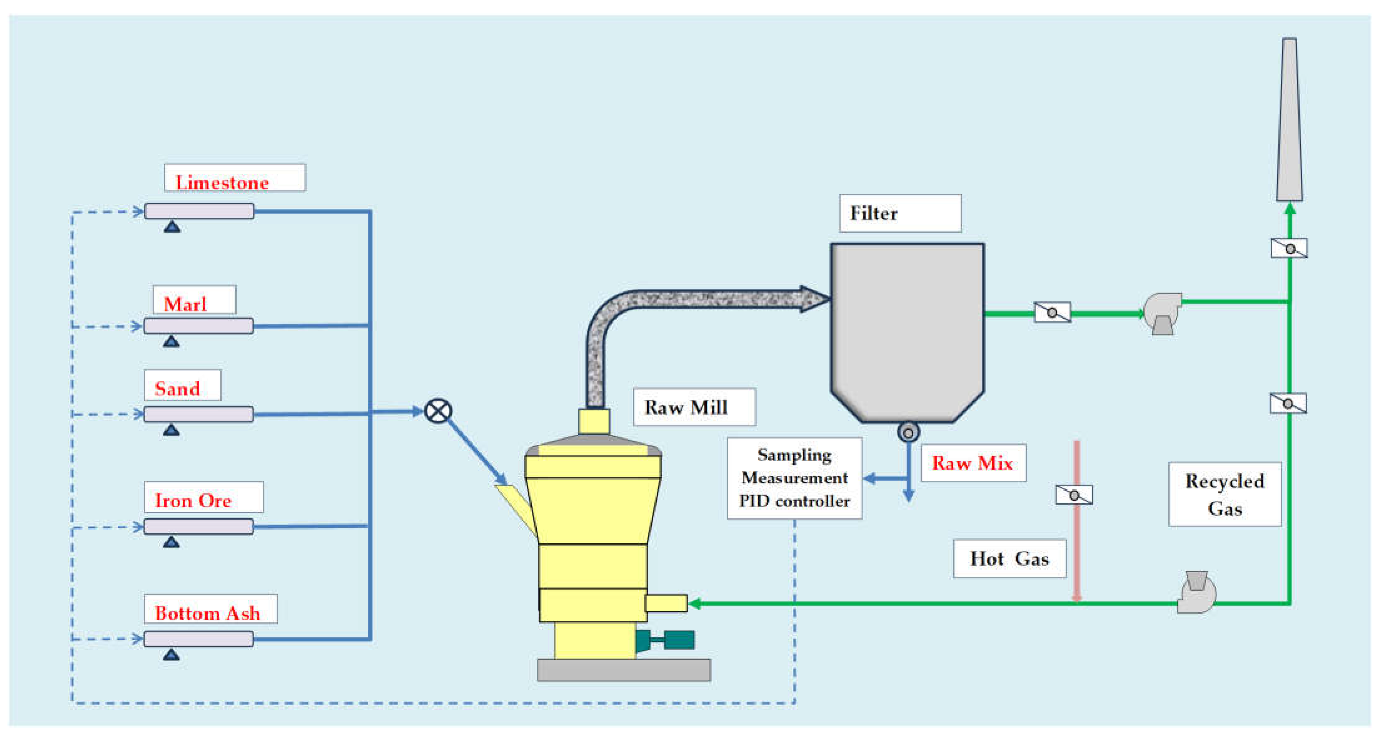
2.1. Process Description

The traditional method of producing reactive clinker involves preparing a raw mix that meets suitable quality targets with minimal variance. In a mill producing raw meal (RM), composition control and regulation are primarily accomplished by adjusting the weight feeders based on the difference between the chemical moduli of the raw meal at the mill outlet and their target values. A detailed description of raw mix production and raw materials analysis can be found in Sections 1 and 2.1 of our previous study [8]. Here, we reiterate some points from [8] for the sake of completeness. Raw meal is milled in a high-capacity vertical mill with a productivity of 400 t/h, equipped with five weight feeders. Figure 1 illustrates a simplified flow sheet [8]: Five feeders deliver raw materials onto a conveyor, which transports them to the mill for grinding. Hot gases carry the ground raw mix to a separator inside the mill, with fines passing through a bag filter to produce raw meal. Most gases recirculate, while kiln exhaust gases help dry the raw mix. The raw meal is then stored in silos for homogenization before being sent to the kiln for clinker production. The control loop regulating the quality of the raw mix at the mill outlet is also indicated in Figure 1 with dotted lines. The input percentages of limestone, sand, iron ore, and bottom ash are independent, denoted as Lim, Sand, Iron, and BA, respectively. The marl content is calculated as follows: Marl = 100 − Lim − Sand − Iron − BA.

In [8], we studied a PID controller with four independent inputs and four outputs; however, in the current study, we focus solely on the controller component that regulates LSF. The value of this modulus is determined from the XRF analysis of an average sample taken regularly from the RM outlet. Equation (1) provides the relationship between LSF and the raw mix oxides [35] (pp. 164–165), where LSF_Mill = LSF in the mill outlet, CaO_Mill = CaO, SiO_2Mill = SiO₂, Al₂O_3Mill = Al₂O₃, and Fe₂O_3Mill = Fe₂O₃.

$${LSF}_{Mill}={\displaystyle \frac{{CaO}_{Mill}·100}{2.8·{SiO}_{2Mill}+1.18·{Al}_2{O}_{3Mill}+0.65·{Fe}_2{O}_{3Mill}}}$$

(1)

2.2. Process Control and PID Design

The open-loop system consists of three consecutive processes: the grinding of raw materials, the preparation of an average sample, and the sampling and measurement of that sample, each with a sampling period of T_s, and corresponding transfer functions G_Mill, G_Av, and G_M, respectively. The process transfer function, G_p, is the product of the three functions mentioned above. The set of Equations (2)–(5) provides these functions in the Laplace domain. A second-order time delay (SOTD) model is used to describe the RM dynamics, as illustrated in Equation (2):

$$G_{Mill}\left(s\right)={\displaystyle \frac{{LSF}_{Mill}\left(s\right)-{LSF}_0}{Lim\left(s\right)-{Lim}_0}}={\displaystyle \frac{k_g}{{\left(1+T_0·s\right)}^2}}·\mathit{exp}\left(-T_D·s\right)$$

(2)

$$G_{Av}\left(s\right)={\displaystyle \frac{{LSF}_{Av}}{{LSF}_{Mill}}}=\left({\displaystyle \raisebox{1ex}{$1$}\!\left/ \!\raisebox{-1ex}{$T_s·s$}\right.}\right)·\left(1-exp\left(-T_s·s\right)\right)$$

(3)

$$G_M\left(s\right)={\displaystyle \frac{{LSF}_M}{{LSF}_{Av}}}=exp\left(-T_M·s\right)$$

(4)

$$G_p\left(s\right)=G_{Mill}\left(s\right)·G_{Av}\left(s\right)·G_M\left(s\right)$$

(5)

k_g is the gain from Lim to LSF_Mill, T₀ is the time constant, T_D is the delay time, and LSF₀ and Lim₀ represent the steady-state values of LSF_Mill and Lim as t→∞ (or s = 0 in (2)). LSF_av is the LSF of the average sample of raw mix, accumulated during the sampling period T_s, while LSF_M is the measured LSF of this sample, which has a delay equal to T_M after the sample is extracted automatically from the sampler. T_M is the measurement time, representing the sum of the time intervals needed for transferring, preparing, and analyzing the sample, as well as calculating the feeders’ settings and transferring them to the weight scales in a closed-loop configuration. The raw mill dynamic parameters were determined using exclusively the process data of Lim and LSF_M by applying the method described in Section 3.2 of [8]. Table 3 in [8] presents values of the vector [k_g, T₀, T_D]^T based on process data covering a period of more than ten years. In this study, we identified datasets with rich dynamics by comparing the actual and calculated LSF values and computing their regression coefficients. Reliable [k_g, T₀, T_D]^T vectors were selected for datasets where the regression coefficient exceeded a specified threshold.

A PID controller regulates LSF_M to be as close as possible to the setpoint LSF_T, using Lim as the control variable and aiming to minimize the error between the process value LSF_M and setpoint (SP). Equations (6) and (7) provide the error e_LSF and the transfer function of the controller, C_LSF, in the Laplace domain.

$$e_{LSF}={LSF}_T-{LSF}_M$$

(6)

$$C_{LSF}={\displaystyle \frac{Lim}{e_{LSF}}}=k_p+{\displaystyle \frac{k_i}{s}}+k_d·s$$

(7)

In Equation (7), k_p, k_i, and k_d represent the proportional, integral, and derivative gains of the PID, respectively. The closed-loop block diagram of the control system is demonstrated in Figure 3 of our previous study [8]. Depending on the magnitude of the absolute value of e_LSF the controller operates with a variable sampling period: if |e_LSF| ≤ 2, then the next T_s = 2 h; otherwise, the next T_s = 1 h. In [8], we discretized the continuous-time controller by applying the incremental form of the PID algorithm using the feedforward approximation for the differences, as represented by Equation (8), in accordance with Åström et al. [18] (pp. 414–421):

$$\Delta Lim=k_p·\left(e_{LSF,n}-e_{LSF, n-1}\right)+k_i·e_{LSF,n}·T_{s,n}+k_d·\left({\displaystyle \frac{e_{LSF,n}-e_{LSF, n-1}}{T_{s,n}}}-{\displaystyle \frac{e_{LSF,n-1}-e_{LSF, n-2}}{T_{s,n-1}}}\right)$$

$${Lim}_n={Lim}_{n-1}+\Delta Lim$$

(8)

The symbol Δ denotes the increment of the controller’s output. The subscripts n, n−1, and n−2 represent the inputs and outputs of the controller at times t_n, t_n−1, and t_n−2. T_s,n = t_n − t_n−1, and T_s,n−1 = t_n−1 − t_n−2.

We implemented the parameterization of the PID by determining the gains [k_p, k_i, k_d]^T using the M-constrained integral gain optimization (MIGO) loop-shaping technique [18] (pp. 206–221), which is part of a family of methods that ensure robustness. Over the last years, there have been various references to this method or similar methods for parameterizing classical and fractional PID controllers in several fields [22,24,36,37,38,39,40]. We provided a detailed description of the MIGO loop-shaping technique for tuning the PID controller of the raw mix in a raw mill in Appendix A of [8].

3. PID Auto-Tuner Design Using ANNs

The design of the robust gain-scheduled PID controller for regulating the raw-mix LSF, as described in [8], is based on three pillars: (1) calculating mill dynamics using exclusively industrial data, (2) parameterizing the controller to meet robustness criteria, and (3) enhancing performance through simulation. The steps (1) and (2) are described in Section 3 of [8], while the simulator algorithm is detailed in Section 4.2 of [8]. The simulator considers an RM operation period T_Op = 200 h and accounts for the uncertainties in the chemical composition of two primary raw materials: limestone and marl. Limestone and marl compositions remain constant for random time intervals T_Lim and T_Marl, bounded by low and high limits T_Min, and T_Max: T_Min ≤ T_Lim ≤ T_Max and T_Min ≤ T_Marl ≤ T_Max. Then, the simulation introduces a step change to the composition of each material, followed by a new interval of constant composition for each, until the operation time equals T_Op. We studied two disturbance periods using the simulator: [T_Min, T_Max] = [6 h, 10 h] and [12 h, 16 h]. High-performance PIDs for a wide range of RM dynamic parameters—k_g, T₀, and T_D—have been determined through simulations that utilize the minimization of the LSF standard deviation as a criterion, resulting in tables where each [k_g, T₀, T_D]^T vector corresponds to a vector of PID gains [k_p, k_i, k_d]^T. Since the PID operates with variable sampling periods of T_s = 2 h and T_s = 1 h, as analyzed in Section 2.2, we calculated two vectors of optimal gains corresponding to each T_s. The auto-tuner has been designed using the optimal PID gains computed from the simulator by applying the intensive disturbance period ranging from 6 to 10 h to enhance robustness. Table S1 presents all the vectors [k_g, T₀, T_D]^T along with the optimal PIDs for T_s = 2 h and T_s = 1 h. This table is a fundamental tool for the gain-scheduled PID control of LSF. The disadvantage is that, for values of [k_g, T₀, T_D]^T that fall between the established values in the table, rounding to the nearest dynamic set of values or linear interpolation is required. Furthermore, significant nonlinearities can be observed between the PID gains and the dynamic parameters. Therefore, continuous functions are necessary to express the relationships between [k_g, T₀, T_D]^T and [k_p, k_i, k_d]^T. A powerful approach to developing the auto-tuner for the PID control of the raw mix is the use of artificial neural networks (ANNs).

3.1. ANN Design and Structure

The inputs and outputs of the developed ANN model are the vectors [k_g, T₀, T_D]^T and [k_p, k_i, k_d]^T from Table S1. Therefore, since each PID gain requires an ANN to express its relationship with the dynamic parameters, three ANNs are necessary. Each ANN contains one hidden layer, in which the number of nodes, (N_N), should be optimized to achieve the minimum test error and maximum generalization, ensuring that the neural network produces reasonable outputs for inputs not encountered during training [41]. The sigmoid function serves as the activation function for each node, a method that we have employed in the construction of neural networks across various fields [15,42].

Based on the implementation of the MIGO method presented in Appendix A of [8], the PID gains are functions of the RM dynamic parameters. However, the differential gain also serves as an additional input for the calculation of k_p and k_i. Therefore, the ANN that calculates and predicts k_d has three inputs, while the ANNs used for predicting k_p and k_i have four inputs. Table S1 contains 490 rows of inputs and outputs. Eighty percent of these rows (392 datasets) have been randomly selected as the training set, while the remaining 20% (98 datasets) constitute the test set. After selecting the training and test sets, our software creates a copy of the initial matrix, where the first 392 rows constitute the training set and the remaining 98 rows belong to the test set. For each ANN and number of nodes, our algorithm continuously selects training and test sets to ensure that the test error converges to a constant value. This process is based on a technique that generates a random sequence of 392 numbers ranging from 1 to 490, continuing until the average test error reaches a stable value within a small tolerance. To avoid overfitting of the ANNs, we employed a weight decay—or L2 regularization—methodology [43,44], which is described in details in [15]. Three ANNs have been developed for the PID gains corresponding to each sampling period. Each ANN has been constructed by employing the following set of equations:

Normalization of input variables in the input layer and normalization of the output variable of each ANN:

$${XN}_{IK}={\displaystyle \frac{X_{IK}-X_{I,MIN}}{X_{I,MAX}-X_{I,MIN}}} , I=1 to N_I ; {YN}_K={\displaystyle \frac{Y_K-Y_{MIN}}{Y_{MAX}-Y_{MIN}}}, K=1 to N_{Tot}$$

(9)

N_I represents the number of input variables for each ANN, where N_I = 3 for the ANN predicting k_d and N_I = 4 for the ANNs predicting k_p and k_i. N_Tot = 490 is the total number of datasets. X_IK denotes the input variable for each ANN, where I = 1, 2, 3 correspond to k_g, T₀, and T_D, respectively, while I = 4 corresponds to k_d. X_I,Min, Y_Min, X_I,Max, and Y_Max are the minimum and maximum values of each input and output variable across the total number of datasets.

Inputs to the hidden layer and activation function:

$$Z_{JK}=\sum _{I=0}^{N_I}{W}_{IJ}·{XN}_{IK}; \sigma \left(Z_{JK}\right)={\displaystyle \frac{1}{1+\mathit{exp}\left(-Z_{JK}\right)}}, J=1 to N_N,K=1 to N_{Train} or N_{Test}$$

(10)

W_IJ denotes the synaptic weight between the input variable I and the node J. XN_0K = 1, to account the bias. Z_JK is the input variable to the sigmoid activation function σ of the node J. N_N represents the number of nodes within the hidden layer. N_Train = 392 is the count of the training dataset, while N_Test = N_Tot − N_Train is the count of the test dataset. The set of Equation (10) is applied to both the training and test datasets.

Output layer:

$${YN}_{K, Train}=\sum _{J=1}^{N_N}{V}_J·\sigma \left(Z_{JK}\right), K=1 to N_{Train}; {YN}_{K, Test}=\sum _{J=1}^{N_N}{V}_J·\sigma \left(Z_{JK}\right), K=1 to N_{Test}$$

(11)

ANN output denormalization:

$$\begin{gathered} Y_{K, Train}=Y_{MIN}+{YN}_{K, Train}·\left(Y_{MAX}-Y_{MIN}\right), K=1 to N_{Train} ; \\ {Y}_{K, Test}=Y_{MIN}+{YN}_{K, Test}·\left(Y_{MAX}-Y_{MIN}\right), K=1 to N_{Test} \end{gathered}$$

(12)

V_J is the synaptic weight from each ANN node J to the normalized output. YN_K,Train, YN_K,Test, Y_K,Train, and Y_Test represent the normalized and denormalized outputs of the ANN for the Kth set of input variables in the training and test datasets, respectively.

The variables that need to be determined are the synaptic weights W_IJ and V_J, where I = 0 to N_I and J = 1 to N_N. Therefore, the total number of independent variables is M = (N_I + 1)·N_N + N_N = (NI + 1)·(N_N + 1). Equations (13) and (14) provide the training and test errors, s²_res,Train and s²_Test, respectively, as well as the objective function, of, to be minimized.

Training error and objective function:

$$s_{res,Train}^2=\sum _{K=1}^{N_{Train}}{\displaystyle \frac{{\left(Y_{K,Train}-Y_K\right)}^2}{N_{Train}-M}} ; of=s_{res,Train}^2+\lambda ·\left(\sum _{J=1}^{N_N}\sum _{I=0}^{N_I}{W}_{IJ}^2+\sum _{J=1}^{N_N}{V}_J^2\right)$$

(13)

Test error:

$$s_{Test}^2=\sum _{K=1}^{N_{Test}}{\displaystyle \frac{{\left(Y_{K,Test}-Y_{NTrain+K}\right)}^2}{N_{Test}}}$$

(14)

The objective function incorporates the coefficient of the weight decay term, λ, through the use L2 regularization. The parameter λ requires optimization to enhance the generalization capability of the ANN under study. For a specified λ value, the optimal parameters that minimize the objective function are obtained using the Levenberg–Marquardt technique, which has proven to be effective in training ANNs [45,46,47]. Equation (13) indicates that the objective function, utilizing the training dataset, depends on the values of both N_N and λ. As a result, the optimal weights, W_ij and V_j, obtained through the Levenberg–Marquardt method, are influenced by these N_N and λ values. The test error, derived from Equation (14), is a function of these weights and, consequently, of both N_N and λ. For each ANN, the optimal number of nodes and the weight decay term are not predetermined; instead, they are selected based on the minimization of the test error.

Figure 2 presents the configuration of the three ANNs used to predict the vectors [k_p, k_i, k_d]^T based on [k_g, T₀, T_D]^T data. The output of the k_d ANN serves as an input for the k_p and k_i ANNs, indicating that these two ANNs consist of two hidden layers, with the first layer being the one belonging to the k_d ANN. The structure presented in Figure 2 indicates the k_d ANN is independent of the other two, while the k_p and k_i ANNs are independent of each other but utilize the output of the k_d ANN as an input. Therefore, treating the system of equations as a typical nonlinear regression problem, the solution begins with the k_d ANN and continues with the two remaining ANNs.

Our algorithm employs an iterative methodology to optimize both the number of nodes in the hidden layer of each ANN and the value of λ:

(1)

A training set and the corresponding test set are selected.

(2)

For a specified λ and number of nodes N_N, the weights of the ANN are optimized by minimizing the objective function, and both the training and test errors are computed.

(3)

Steps (1) and (2) are repeated, averaging each new training and test error with the previous results.

(4)

The algorithm iterates through steps (1) to (3) for a total of 1000 training and test sets to ensure that the test error converges to a constant value.

(5)

Steps (1) to (4) are performed across a range of λ and N_N values to identify the optimal λ and N_N that yield the minimum average test error.

The Levenberg–Marquardt technique is implemented in step (2) to minimize the objective function which consists of two terms: the training error and the L2 regularization term, and is a function of specific values of NN and λ. The nested steps (3) to (5) determine the average test errors across a range of NN and λ. Finally, the optimal values of these two parameters correspond to those that yield the minimum average test error.

3.2. Final Design of the Auto-Tuner

Assessing whether the current PID gains require adjustment by the auto-tuner is an ongoing process consisting of sequentially designed and implemented steps that operate automatically, following the algorithm below:

-

Firstly, our software retrieves the most recent RM quality data—specifically, the raw meal composition and LSF—for which the RM dynamic parameters have not yet been calculated.

-

The dynamic parameters are computed using the algorithm described in Section 3.2 of [8], with significant results being those for which the square root of the adjusted R² is greater than 0.7.

-

The sets of significant dynamic results are divided into consecutive groups of 200 sets, and the size N_s of the remaining most recent group is checked. If N_s < 200, the auto-tuner does not proceed with further action and instead waits for N_s to reach the value 200.

-

When N_s becomes equal to 200, the algorithm computes the average values of k_g, T₀, and T_D for the latest group and compares these averages with the respective mean values of the preceding group, which also has N_s = 200, by calculating the absolute difference between them.

-

If at least one of the three absolute differences exceeds a tolerance of 0.001, the most recent dynamic parameters are considered significantly different from the previous ones, prompting the algorithm to calculate new PID gains. Otherwise, the differences are deemed insignificant, and the auto-tuner retains the previous PID gains.

-

In the event of a significant difference between the latest and the preceding dynamic parameters, the auto-tuner calculates two new sets of PID gains [k_p, k_i, k_d]^T for sampling periods T_s = 1 h and T_s = 2 h, using the ANNs described in Section 3.1. The computation employs the optimal number of nodes, N_N, and weight decay term, λ, as determined by the algorithm of 3.1. The new gains are transferred to the software regulating raw meal quality, either automatically or manually. All new data are saved in the plant’s quality database.

4. Optimization of the ANNs

Optimizing each ANN requires identifying the number of nodes and the weight decay term that yield the minimum average test error, which is calculated after selecting a total of 1000 training and test sets. We first demonstrate that a count of 1000 selections is sufficient for converging the average test error. Figure 3 presents the cumulative test error for sets ranging from 1 to 1000. Figure 3a shows the results for the k_d ANNs with λ = 0, T_s = 1 h, and N_N = 2, 3, 4, 5, 6, while Figure 3b illustrates the results for the k_p ANNs with λ = 0, T_s = 2 h, and N_N = 2, 3, 4, 5. The cumulative errors for all the ANNs converge to constant average test error when the number of sets reaches 1000.

Figure 4 illustrates the average test error of the three ANNs as a function of the number of nodes and λ for T_s = 2 h. In Figure 4b,d,f, it is evident that an optimal weight decay parameter, λ, results in a considerably lower test error than when λ = 0. In the case of the k_p and k_i ANNs, the optimal range of λ is relatively broad, as indicated in Figure 4c,e.

Table 1. Settings of the optimum ANNs.

ANN	Ts, h	NN	λ	Average of Adjusted R2	Std. Dev. of Adjusted R2	Average of R2	Std. Dev. of R2
kd	1	6	2·10−6	0.9520	2.14·10−3	0.9482	9.34·10−3
kd	2	4	1·10−6	0.9597	1.98·10−3	0.9593	7.56·10−3
kp	1	6	3·10−6	0.9695	1.48·10−3	0.9657	7.28·10−3
kp	2	3	2·10−5	0.9359	2.94·10−3	0.9351	1.18·10−3
ki	1	6	1·10−5	0.9617	1.77·10−3	0.9563	8.84·10−3
ki	2	3	3·10−5	0.8036	8.19·10−3	0.8014	3.34·10−3

presents, for each ANN and sampling period, the optimum number of nodes and λ, along with the average and standard deviation of adjusted R² for the training sets and the average and standard deviation of R² for the test sets derived from the 1000 training and test sets selected.

The average values of adjusted R² and R² are quite similar, suggesting that the use of L2 regularization is successful in preventing overfitting across all the developed ANNs. The standard deviation of R² is three to five times larger than that of adjusted R². This discrepancy may be attributed to the fact that the size of the test set population is four times smaller than that of the training set. The final synaptic weights of each optimal ANN have been determined using the complete population of 490 datasets, executing the Levenberg–Marquardt method until the standard error, as defined in Equation (13) for N_Train = N_Tot, is less than or equal to the average test error calculated by the algorithm in Section 3.1.

5. Simulation Studies

5.1. General Description

The proposed auto-tuner’s effectiveness has been assessed using a simulator designed for the raw-mix production process, detailed in Section 4 of [8]. The simulator focuses on the LSF control loop and encompasses analyses of raw materials, key process parameters, and their related uncertainties. The simulator developed in [8] was intended to determine the optimum PID gains based on the process dynamic parameters k_g, T₀, and T_D. The simulation to be analyzed utilizes the optimal gains obtained from the implementation of ANNs. It then compares two long-term RM operations using the following PID configurations: (a) PID with constant gains, which are initially optimal but do not adjust when changes in dynamic parameters are detected, and (b) PID with variable gains, which adapt after the detection of changes in the dynamic parameters.

The simulator utilizes pairs of limestone and marl compositions, the same ones used in the simulation described in [8], with CaO content presented in

Table 2. Chemical composition combinations for limestone and marl.

Combination	1	2	3	4	5	6	7	8	9	10
%CaO Limestone	54.0	54.5	55.0	55.0	55.0	55.0	55.0	55.0	55.0	55.0
%CaO Marl	19.3	18.0	17.4	16.2	15.0	14.2	13.3	12.3	11.2	9.0
kg	3.95	4.10	4.17	4.30	4.42	4.51	4.60	4.71	4.82	5.05

. The gains k_g and the remaining oxides of limestone and marl have been computed by implementing the equations provided in [8].

The mill operates for T_Op = 2000 h with a constant average composition of limestone and marl, selected from the pairs listed in Table 2. Small random disturbances, normally distributed, are added to the mean CaO content of each raw material, lasting for time periods T_Lim h and T_Marl h, where T_Min ≤ T_Lim ≤ T_Max and T_Min ≤ T_Marl ≤ T_Max. Both integers T_Lim and T_Marl are also randomly selected, belonging continuously to the interval [T_Min, T_Max] = [6 h, 10 h]. The dynamic parameters T₀ and T_D maintain constant average values throughout T_Op and are perturbed around these values with small random disturbances lasting T_Dyn h, where the integer T_Dyn is randomly selected from the interval [T_DynMin, T_DynMax] = [20 h, 28 h]. Section 4.2 of [8] provides details on the statistics of the selections mentioned above. The sampling period T_s set to 1 h, with the sample representing the average raw meal produced during that hour, and the PIDs selected correspond to T_s = 1 h. The RM operates for N_Op time intervals, each lasting T_Op hours. At the beginning of each T_Op period, at least one of the dynamic parameters—k_g, T₀, or T_D—changes. The modification in k_g is determined by choosing a different limestone and marl composition from Table 2. Consequently, N_Op changes in process dynamics are implemented.

In the case where the auto-tuner is off, the PID has constant gains. The initial [k_p, k_i, k_d]^T is computed using the ANNs and the [k_g, T₀, T_D]^T from the first T_Op period. For the subsequent N_Op − 1 intervals, the PID gains remain constant. It is assumed that the process dynamics were the same prior to the start of the first T_Op period, allowing the dynamic parameters to be calculated using the algorithm outlined in Section 3.2 of [8]. When the auto-tuner is activated, the PID gains are determined for each i_AT interval, where i_AT ranges from 2 to N_Op, using the ANNs and the dynamic parameters of each interval. However, a specific number of hourly samples are necessary for the algorithm to identify the new dynamics. The simulator assumes that the first T_F hours of each i_AT interval are required to detect and compute the new dynamics. The PID operates for T_F hours using the gains from the previous interval (i_AT − 1) and for T_Op − T_F hours with the gains from the current interval (i_AT). The variable T_F is a parameter whose impact on the LSF variance will be examined.

5.2. Initial Simulations

Initially, the simulator was applied for N_Op = 10, employing all the combinations of limestone and clay compositions listed in Table 2, along with specified values of T₀ and T_D.

Table 3. Settings of the initial simulation.

	Series 1 (S1)					Series 2 (S2)
iAT	%CaO Lim.	%CaO Marl	kg	T0	TD	%CaO Lim.	%CaO Marl	kg	T0	TD
1	54.0	19.3	3.95	0.30	0.30	55	14.2	4.51	0.30	0.30
2	54.5	18	4.1	0.30	0.30	55	14.2	4.51	0.30	0.31
3	55	17.4	4.17	0.30	0.30	55	14.2	4.51	0.30	0.32
4	55	16.2	4.3	0.30	0.30	55	14.2	4.51	0.30	0.33
5	55	15	4.42	0.30	0.30	55	14.2	4.51	0.30	0.34
6	55	14.2	4.51	0.30	0.30	55	14.2	4.51	0.30	0.35
7	55	13.3	4.6	0.30	0.30	55	14.2	4.51	0.30	0.36
8	55	12.3	4.71	0.30	0.30	55	14.2	4.51	0.30	0.37
9	55	11.2	4.82	0.30	0.30	55	14.2	4.51	0.30	0.38
10	55	9	5.05	0.30	0.30	55	14.2	4.51	0.30	0.39

presents two series of simulations consisting of ten consecutive datasets (i_AT = 1 to 10). In the first series, the ten compositions are utilized and sorted so that the k_g values are in ascending order, while T₀ and T_D remain constant. In the second series, T_D increases from 0.3 h to 0.39 h in steps of 0.01 h, while k_g and T₀ are held constant. The time to detect the new dynamics per dataset is T_F = 500 h, while T_Op = 2000 h.

Figure 5 illustrates the LSF average standard deviations obtained for each dataset for the two series of simulation (S1 and S2) with the auto-tuner (AT) both off and on. The average standard deviation is the mean of the population of standard deviations computed from all iterations for each dataset, as described in the simulation algorithm in [8].

In both series, when the auto-tuner is activated, the average standard deviation of the LSF is maintained between 2.7 and 3.0. This situation proves the robustness of the auto-tuner. However, when the auto-tuner is deactivated in the first series—where only the raw materials composition changes—the standard deviation increases rapidly when the compositions of one dataset become significantly different from those of the first dataset (for i_AT ≥ 9). This indicates that the PID parameters from the first dataset are insufficient for effectively regulating the process. In the second series, with the auto-tuner off, the standard deviation begins to increase early (i_AT ≥ 4), indicating that the PID gains from the first dataset, which are designed for a specific range of time delays, are ineffective in regulating a process with delays significantly different from those for which they were designed. We can identify three sources that create changes in the time constants of the process dynamics: (a) a change in the hardness of the raw materials, (b) a modification of the fineness target for the raw mix, which leads to a change in the separator speed and, consequently, to the circulating load of the mill, and (c) a gradual change in the condition of the grinding media in the mill. Finally, the initial simulations suggest that the actions of the auto-tuner keep the LSF variance at low levels, which cannot be ensured when the PID gains remain constant.

5.3. Full Simulation

To gain a better understanding of the benefits that the auto-tuner provides compared to a PID with constant gains, we conducted a more detailed analysis that relies on the random generation of the three dynamic parameters. The procedure is as follows:

• A total of 20 consecutive datasets (N_Op = 20) are used, with T_Op = 2000 h and T_F = 500 h, 750 h, and 1000 h with the auto-tuner activated, and the same datasets with the auto-tuner deactivated.
• For each dataset, one of the ten combinations of limestone and clay compositions listed in Table 2 is randomly and consecutively selected. The corresponding gain (k_g) for each pair of compositions is also provided in Table 2.
• For each consecutive dataset the T₀ and T_D values are determined using the random generator, such that T₀ ∈ [0.3 h, 0.5 h] and T_D ∈ [0.3 h, 0.5 h].
• The simulator executes all the steps outlined in Section 5.1 and Section 5.2 for the 20 datasets.
• Afterward, a new group of N_Op datasets is selected, and the steps (1) to (4) are repeated.
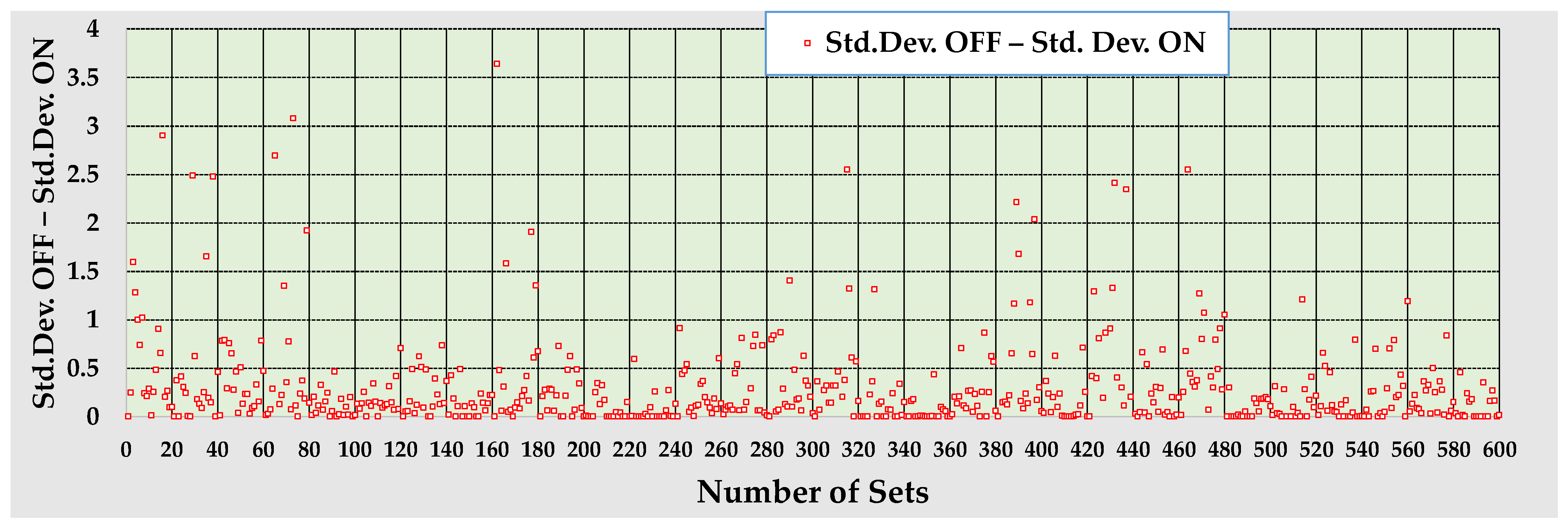
• The procedure continues until a total of 30 groups of N_Op datasets are completed. Therefore, the results are based on 600 datasets.

Figure 6 displays the differential distribution of the LSF average standard deviation for the 600 datasets, calculated as described in Section 5.2, when the auto-tuner is either activated or deactivated. A partitioning of 0.25 has been chosen for the standard deviations on the X-axis. Each point represents the percentage of the standard deviation population that occurs between the current coordinate on the standard deviation axis and the next coordinate.

The distribution of the standard deviations when the auto-tuner is on forms a bell-shaped curve with a sharp peak. The standard deviations greater than 3.75 are approximately 1.5% for T_F = 500 h, 2.5% for T_F = 750 h, and 3.2% for T_F = 1000 h. In contrast, the corresponding distribution when the auto-tuner is off is strongly skewed to the right, featuring an extended tail. Approximately 20.5% of the standard deviations are greater than 3.75, and 4.3% are greater than 5.0. When T_F increases from 500 h to 1000 h, there is a slight worsening of the standard deviations; however, their distribution remains consistently bell-shaped with a small tail.

The reasons for the significant superiority of the PID controllers when the auto-tuner is activated compared to the off condition should be explored through a thorough analysis of the results from the 30 groups of datasets. Figure 7 presents the differences between the standard deviations when the auto-tuner is off and on (DiffStd = Std. Dev. OFF − Std. Dev. ON), with T_F = 500 h, across all 600 datasets. Each difference corresponds to the same raw materials composition and the same types of disturbances. The average raw materials composition is kept constant for each dataset. As mentioned in Section 5.1, when the auto-tuner is off, the PID is optimal for the first dataset but remains constant for the subsequent 19 datasets. In contrast, when the auto-tuner is active, the PID gains are adjusted 500 h after the startup of each dataset, regulating the LSF for a total of 2000 h, except for the last dataset, where the PID with the modified gains operates for 1500 h.

The conclusions for the difference DiffStd are the following:

• The nonnegative difference varies from 0 to approximately 3.0. There are groups of 20 datasets where DiffStd remains consistently below 0.5, as well as groups where DiffStd is higher than 0.5 for a non-negligible number of datasets.
• DiffStd is equal to zero for the first dataset of each group and stays around zero for approximately 20% of the datasets, including the initial 30 zeros. The reason that sometimes the constant PID seems to work well is the random generation of the dynamic parameters k_g, T₀, T_D. If randomly occurs that the range of each parameter over the 20 datasets is short and the initial parameters are in the middle of these ranges, then the initial PID can indeed function effectively for all 20 datasets. In such cases, the auto-tuner will also make only slight adjustments to the PID gains. Examples of this behavior can be observed in datasets 341–360 and 481–500. Our auto-tuner design algorithm, as described in Section 3.2, predicts this scenario.
• Table 4. Cumulative distribution of the datasets for DiffStd values greater than 0.2.

  DiffStd ≥	0.2	0.35	0.5	0.75	1.0	1.25	1.5
  % of datasets	43.8	27.2	19.2	12.6	8.6	7.6	5.8

  provides the cumulative distribution of the datasets for DiffStd values greater than 0.2. The statistics have been generated from the data displayed in Figure 7.

For approximately 44% of the datasets, the auto-tuner results in a reduction in the LSF standard deviation by at least 0.2. The results shown in the right part of the table are more critical: DiffStd exceeds 1 in about 8.6% of the datasets and is greater than 1.5 in approximately 5.8% of the datasets. The notable advantage of the auto-tuner is the near-complete elimination of standard deviations greater than four, as shown in Figure 6. It is important to point out that each dataset encompasses 2000 h of RM operation. Assuming that the raw mill of a full production plant operates 20 h per day and 300 days per year, 2000 h equate to approximately four months of operation. Under the condition that the PID is poorly tuned due to changes in process dynamics without adjustments to the PID gains, combined with low raw mix volumes in the stock silo, the high standard deviation of the LSF in the kiln feed can result in instability in kiln operation and negatively affect clinker quality. This might lead to an increase in free lime or a decrease in calcium trisilicate. Furthermore, it can cause a reduction in the use of alternative fuels and raw materials as a means to compensate for the deterioration in quality.

6. Long-Term Operation of the Control System Using the Auto-Tuner

The adaptive controller regulating the LSF using the auto-tuner outputs is in continuous operation at the Heidelberg Materials Devnya cement plant. It manages the quality of the raw mix produced by a vertical mill with a capacity of 400 tons per hour. Once mixed in a silo, the raw meal is fed into a kiln that produces 4400 tons of clinker per day. As described in [8], the controller functions with a variable sampling period, alternating between T_s = 2 h and 1 h, depending on the difference in the raw meal LSF from LSF_T. We grouped the sample population into intervals of 200 h of operating time to minimize the effect of set point changes on the LSF standard deviations as much as possible. We applied the Shewhart control charts [48] (pp. 8–9), particularly the s-charts, to investigate the range of standard deviations in the long term. The central line, along with the upper and lower control limits (CL, U_CL, and L_CL, respectively), is provided by Equation (15), where s_i is the standard deviation of each group of results with a duration of 200 h, M_G is the total number of groups, and a_G is equal to 6. To account for the maximum likely range of standard deviations observed over the long term, we used an expansion coefficient of a_G = 6, rather than the a_G = 3 typically used in standard Shewhart charts. In this case, 99.73% of the normal population is covered. The parameter c₄, used to calculate the margins of CL when a_G = 1, is calculated via the Formula (16) using the Gamma function [49]. N_G is the average of the samples taken during the M_G groups of 200 h of operating time with variable sampling times. In the studied period, N_G = 122.

$$CL={\displaystyle \raisebox{1ex}{$\sum _{i=1}^{M_G}{s}_i$}\!\left/ \!\raisebox{-1ex}{$M_G$}\right.} , i=1 to M_G, L_{CL}=s_i\left(1-a_G·{\displaystyle \raisebox{1ex}{$\sqrt{1-c_4^2}$}\!\left/ \!\raisebox{-1ex}{$c_4$}\right.}\right) , U_{CL}=s_i\left(1+a_G·{\displaystyle \raisebox{1ex}{$\sqrt{1-c_4^2}$}\!\left/ \!\raisebox{-1ex}{$c_4$}\right.}\right)$$

(15)

$$c_4=\sqrt{{\displaystyle \frac{2}{N_G-1}}}·{\displaystyle \frac{\Gamma \left(\raisebox{1ex}{$N_G$}\!\left/ \!\raisebox{-1ex}{$2$}\right.\right)}{\Gamma \left(\raisebox{1ex}{$\left(N_G-1\right)$}\!\left/ \!\raisebox{-1ex}{$2$}\right.\right)}}$$

(16)

Figure 8 displays the s-chart of the LSF standard deviations, including 16,800 h of RM operation. The calculated statistics are CL = 2.52, L_CL = 1.55, and U_CL = 3.50. Only seven out of the 84 groups present a standard deviation higher than 3.5. This case highlights operational periods of 200 h during which disturbances occur at much higher frequencies compared to those experienced in the remaining operating time. Approximately 80% of the groups exhibit a standard deviation less than or equal to 2.84, providing strong evidence of the robustness of the auto-tuner. In [8], we calculated the reproducibility of LSF, s_R, by applying the cement standard related to XRF analysis [50] and the statistical standard for uncertainty expression [51]. We found that s_R is equal to 1.44. The L_CL is very close to this value, suggesting that even with the implementation of a high-precision XRF analysis, achieving a lower standard deviation is challenging. Among the 84 groups analyzed, 77 have a standard deviation that is below the U_CL. This indicates strong performance; with a low mixing ratio of the silo (defined as StdDev_SiloIn/StdDev_SiloOut) equal to 2, the LSF standard deviation in the kiln feed is equal to or less than 1.75, which is very close to the reproducibility of the analysis. This means that any disturbance in the RM feed practically disappears.

Figure 9 depicts the control chart of the quarterly standard deviations of LSF for the raw mix in the kiln feed, starting from 2021. The central line, along with the upper and lower control limits, has been computed using Equations (15) and (16). We used an expansion coefficient a_G equal to 3. The calculated statistics are CL = 1.62, L_CL = 1.43, and U_CL = 1.80. The average number of samples collected during the analyzed quarters is N_G = 338. The kiln feed results confirm the conclusions derived from the analysis of standard deviations in the RM outlet. Only three out of the 13 results have values higher than 1.8, while the central line is equal to 1.62, which is close to the method’s reproducibility. The lower control limit (L_CL) is near the estimated method’s reproducibility (1.44), and four out of the 13 results lie between 1.28 and 1.41, indicating excellent laboratory performance.

The results of the LSF standard deviation indicate that utilizing a strong tuning method, like loop-shaping, alongside an auto-tuner for PID gains based on artificial neural networks (ANNs), guarantees the successful long-term implementation of an adaptive PID controller, as it effectively manages process uncertainties and disturbances.

7. Conclusions

In the earlier sections, we introduced an effective method for creating a robust auto-tuner for PID control of the LSF of the raw mix using artificial neural networks. This auto-tuner and the robust PID controller examined in a prior study [8] form an integrated system capable of compensating for changes in process dynamics and ensuring low long-term variance of the LSF, which is the most significant modulus of the raw meal. This represents the technical innovation of this study, as it is difficult to find in the literature a self-tuned PID controller for raw mix, especially designs that combine both the PID controller and the auto-tuner. The main conclusions of this study are as follows:

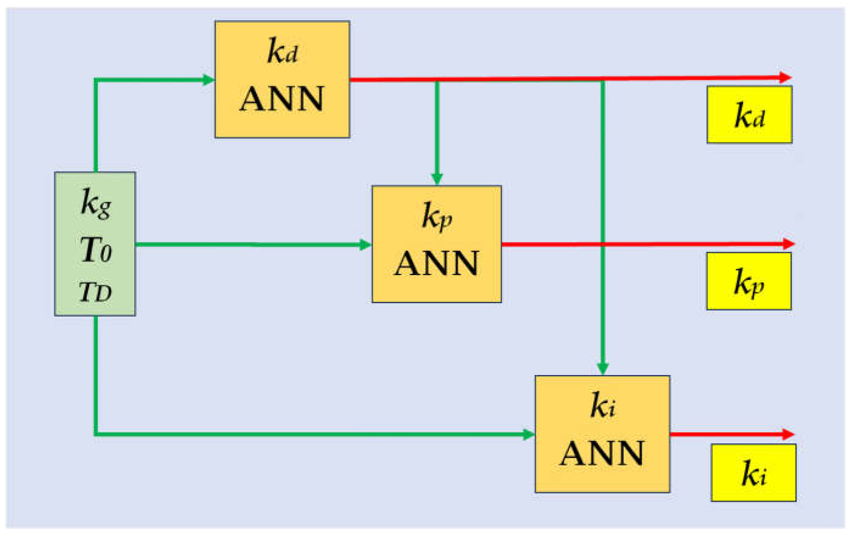
• The three developed ANNs correlate each triad of dynamic parameters k_g, T₀, and T_D to their optimum PID gains k_p, k_i, and k_d. Each ANN contains a single hidden layer. The ANN predicting k_d has three inputs, and its output serves as an additional input to the ANNs predicting k_p and k_i. The number of nodes in each ANN requires optimization for both sampling periods, using the minimization of the test error as the criterion. Consequently, the total number of the ANNs to be optimized for the two sampling periods is six. The optimal parameters that minimize the objective function are determined using the Levenberg–Marquardt technique.
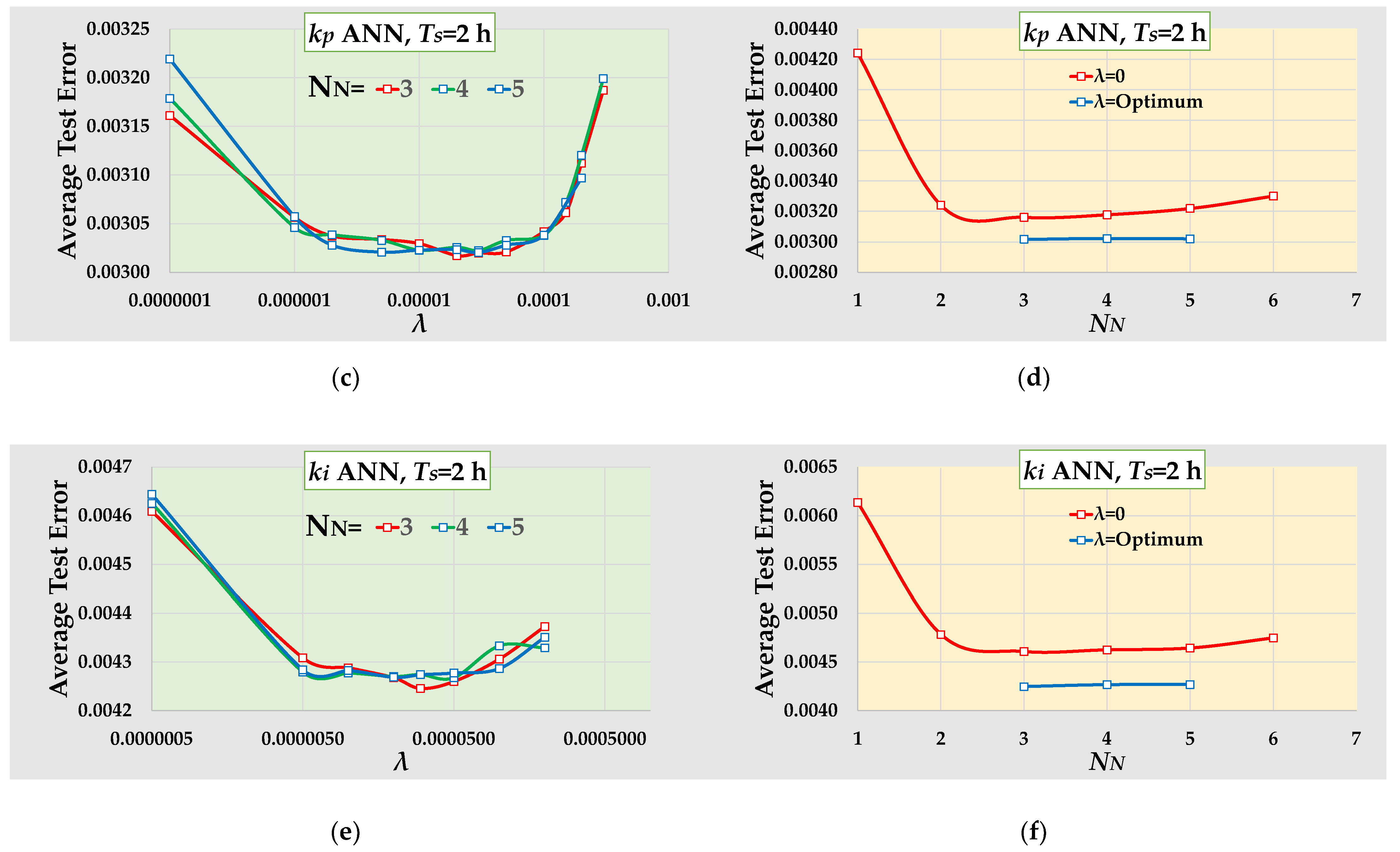
• The L2 regularization methodology has proven to be highly effective in preventing overfitting. The value of the weight decay term λ, which requires optimization, significantly impacts the test error. Our algorithm optimizes both the number of nodes and the weight decay term. The average values of adjusted R² of the training error and R² of the test error are quite similar, suggesting that the use of L2 regularization is successful in preventing overfitting across all the developed ANNs.
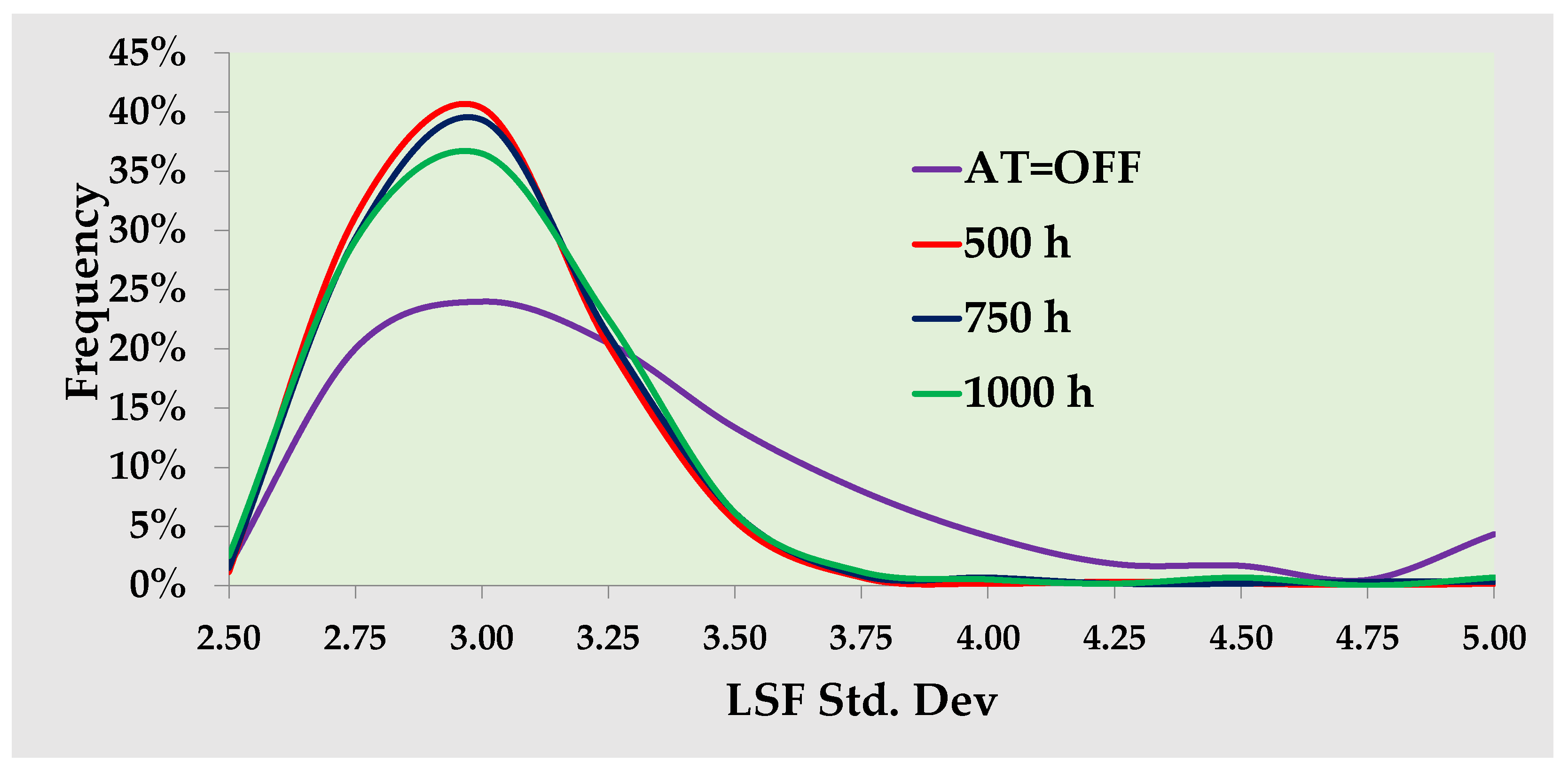
• Our full simulation of the long-term operation of the raw mill, where the LSF is regulated by a PID controller and the auto-tuner is either activated or deactivated, indicates that the standard deviation when the auto-tuner is off is greater than when it is on. The difference between the two standard deviations exceeds 1 in about 8.6% of the datasets. If the PID is poorly tuned due to changes in process dynamics without adjustments to the PID gains, combined with low raw mix volumes in the stock silo, the high standard deviation of the LSF in the kiln feed can lead to instabilities in kiln operation and lower clinker quality. This situation can cause a decreased utilization of alternative fuels and raw materials as a means to address the decline in quality.
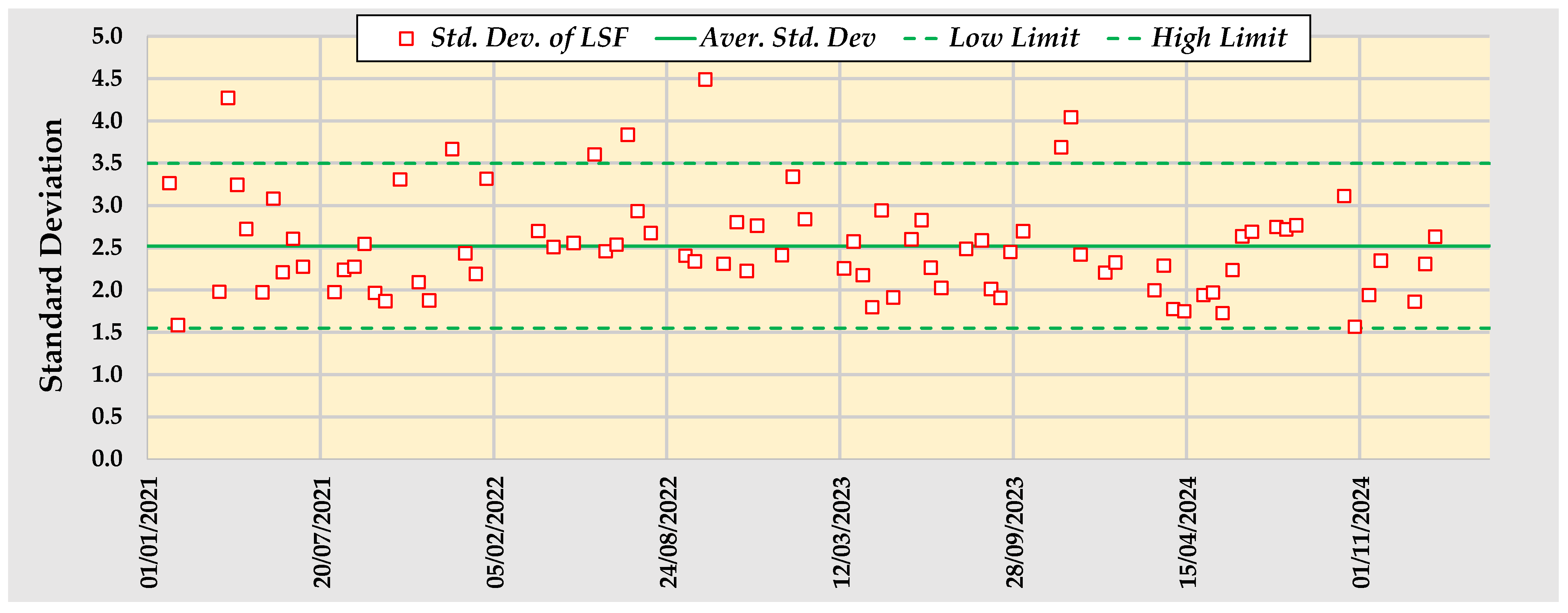
• The long-term industrial operation of our control system using the auto-tuner demonstrates that an average standard deviation of the LSF equal to 2.5 has been achieved, with less than 10% of the result datasets exhibiting a standard deviation higher than 3.5. This indicates a high level of long-term performance for the integrated control technique. Since more than 90% of the standard deviations are less than 3.5, and for a low mixing ratio of the silo equal to 2, the LSF standard deviation in the kiln feed is equal to or less than 1.75, which is very close to the reproducibility of the analysis. The actual results of LSF standard deviation in the kiln feed support this conclusion. Ten out of the thirteen LSF standard deviations from samples collected quarterly are less than or equal to 1.8. This indicates that any disturbance in the raw meal feed practically disappears.

The analysis of the industrially operating integrated control system demonstrates the following:

• The utilization of a robust tuning method, such as loop-shaping, in conjunction with a robust auto-tuner for PID gains based on artificial neural networks (ANNs), ensures the successful long-term implementation of an adaptive PID controller for quality control of the raw mix, effectively managing process uncertainties, disturbances, and changes.
• In conclusion, integrating traditional, well-established tools with newer advanced techniques can yield innovative solutions.

References

1. Kawai, S.; Koike, Y. Real Time Computer Control of Cement Industry. In Real Time Microcomputer Control of Industrial Processes. Microprocessor-Based Systems Engineering; Tzafestas, S.G., Pal, J.K., Eds.; Springer: Dordrecht, The Netherlands, 1990; Volume 5, pp. 435–480. [Google Scholar] [CrossRef]
2. Walther, T. Digital transformation of the global cement industry. In Proceedings of the 2018 IEEE-IAS/PCA Cement Industry Conference (IAS/PCA), Nashville, TN, USA, 6–10 May 2018. [Google Scholar] [CrossRef]
3. 10 Ways AI Is Being Used by the Cement Industry. 2024. Available online: https://digitaldefynd.com/IQ/ai-in-cement-industry/ (accessed on 11 January 2025).
4. Swain, A.K.; Subuthi, B. Computer Control of Cement Raw Mill with an Improved Material Mix Control Scheme. Available online: http://dspace.nitrkl.ac.in/dspace/bitstream/2080/487/1/Computer-1996.pdf (accessed on 14 January 2025).
5. Araromi, D.O.; Odewal, S.A.; Hamed, J.O. Neuro-fuzzy modelling of blending process in cement plant. Adv. Sci. Technol. Res. J. 2015, 9, 27–33. [Google Scholar] [CrossRef] [PubMed]
6. Tiryaki, A.E.; Kozan, R.; Adar, N.G. Mathematical modeling of a cement raw-material blending process using a neural network. Mater. Technol. 2016, 50, 485–490. Available online: http://mit.imt.si/izvodi/mit164/tiryaki.pdf (accessed on 14 January 2025).
7. Zhang, Z.; Nielsen, M.K.; Muralidharan, G.; Hørsholt, S.; Jørrgensen, J.B. Model Predictive Control for Blending Processes in Cement Plants. IFAC-PapersOnLine 2022, 55, 483–488. Available online: https://www.sciencedirect.com/science/article/pii/S2405896322008965 (accessed on 14 January 2025). [CrossRef]
8. Tsamatsoulis, D. Robust Adaptive Control System of Variable Sampling Period for Cement Raw Mix Quality Control. ChemEngineering 2024, 8, 113. [Google Scholar] [CrossRef]
9. Tsamatsoulis, D.; Zlatev, G. PID parameterization of Cement Kiln Pre-Calciner Based on Simplified Modeling. Available online: https://www.naun.org/main/NAUN/neural/2016/a142016-083.pdf (accessed on 14 January 2025).
10. Zhang, J.; Meng, Q.; Yu, H. The Application of Dynamic Matrix Control in the Grate Cooler. In Proceedings of the 2017 IEEE 2nd Advanced Information Technology, Electronic and Automation Control Conference, Chongqing, China, 25–26 March 2017; pp. 2630–2633. Available online: https://ieeexplore.ieee.org/document/8054501 (accessed on 14 January 2024).
11. Seraj, M.; Shooredeli, M.A. Data-Driven Predictor and Soft-Sensor Models of a Cement Grate Cooler Based on Neural Network and Effective Dynamics. In Proceedings of the 2017 Iranian Conference on Electrical Engineering, Tehran, Iran, 2–4 May 2017; pp. 726–731. Available online: https://ieeexplore.ieee.org/document/7985134 (accessed on 14 January 2025).
12. Meng, Q.; Wang, Y.; Xu, F.; Shi, X. Control strategy of cement mill based on Bang-Bang and fuzzy PID self-tuning. In Proceedings of the 2015 IEEE International Conference on Cyber Technology in Automation, Control, and Intelligent Systems (CYBER), Shenyang, China, 8–12 June 2015; pp. 1977–1981. Available online: https://ieeexplore.ieee.org/document/7288250 (accessed on 14 January 2025).
13. Ma, T.; Li, Z.; Liu, J.; Alkhateeb, A.F.; Jahanshahi, H. A novel self-learning fuzzy predictive control method for the cement mill: Simulation and experimental validation. Eng. Appl. Artif. Intell. 2023, 120, 105868. [Google Scholar] [CrossRef]
14. Pawuś, D.; Paszkiel, S. Research Towards an Optimal Method of Modeling and Regulating a Cement Mill Using AI Algorithms. In Automation 2024: Advances in Automation, Robotics and Measurement Techniques. Lecture Notes in Networks and Systems; Szewczyk, R., Zieliński, C., Kaliczyńska, M., Bučinskas, V., Eds.; Springer: Cham, Switzerland, 2025; Volume 1219, pp. 3–16. [Google Scholar] [CrossRef]
15. Tsamatsoulis, D. Prediction of Cement Compressive Strength by Combining Dynamic Models of Neural Networks. Chem. Biochem. Eng. Q. 2021, 35, 295–318. [Google Scholar] [CrossRef]
16. Åström, K.J. Model Uncertainty and Robust Control, Lecture Notes on Iterative Identification and Control Design, Lund University. 2000. Available online: https://www.researchgate.net/publication/228602986_Model_Uncertainty_and_Robust_Control/ (accessed on 14 January 2025).
17. Rivas-Echeverría, F.; Ríos-Bolívar, A.; Casales-Echeverría, J. Neural Network-based AutoTuning for PID Controllers. Neural Netw. World 2001, 11, 277–284. Available online: https://www.researchgate.net/publication/242777564_Neural_Network-based_AutoTuning_for_PID_Controllers (accessed on 14 January 2025).
18. Åström, K.J.; Hägglund, T. Advanced PID Control; Instrumentation, Systems and Automatic Society: Research Triangle Park, NC, USA, 2006; pp. 112–114, 206–221, 296–297, 414–421. [Google Scholar]
19. Vesely, V.; Ilka, A. Gain-scheduled PID controller design. J. Process Control 2013, 23, 1141–1148. [Google Scholar] [CrossRef]
20. Pavković, D.; Polak, S.; Zorc, D. PID controller auto-tuning based on process step response and damping optimum criterion. ISA Trans. 2014, 53, 85–96. [Google Scholar] [CrossRef]
21. Kim, K.H.; Bae, J.E.; Chu, S.C.; Sung, S.W. Improved Continuous-Cycling Method for PID Autotuning. Processes 2021, 9, 509. [Google Scholar] [CrossRef]
22. Zhao, S.; Liu, S.; De Keyser, R.; Ionescu, C.-M. The Application of a New PID Autotuning Method for the Steam/Water Loop in Large Scale Ships. Processes 2020, 8, 196. [Google Scholar] [CrossRef]
23. Hoshu, A.A.; Wang, L.; Sattar, A.; Fisher, A. Auto-Tuning of Attitude Control System for Heterogeneous Multirotor UAS. Remote Sens. 2022, 14, 1540. [Google Scholar] [CrossRef]
24. Muresan, C.I.; Birs, I.; Ionescu, C.; Dulf, E.H.; De Keyser, R. A Review of Recent Developments in Autotuning Methods for Fractional-Order Controllers. Fractal Fract. 2022, 6, 37. [Google Scholar] [CrossRef]
25. Feliu-Batlle, V.; Sotomayor-Moriano, J.; Rivas-Perez, R. Adaptive Smith Predictor Controller Design for Industrial Processes with Time Varying Time Delay. IFAC-PapersOnLine 2024, 58, 37–42. [Google Scholar] [CrossRef]
26. Qu, S.; He, T.; Zhu, G. Model-Assisted Online Optimization of Gain-Scheduled PID Control Using NSGA-II Iterative Genetic Algorithm. Appl. Sci. 2023, 13, 6444. [Google Scholar] [CrossRef]
27. Berner, J.; Åström, K.J.; Hägglund, T. Towards a New Generation of Relay Autotuners. In Proceedings of the 19th World Congress of the International Federation of Automatic Control, Cape Town, South Africa, 24–29 August 2014; Volume 47, pp. 11288–11293. [Google Scholar] [CrossRef]
28. Åström, K.J.; Hägglund, T. Automatic tuning of simple regulators for phase and amplitude margins specifications. In Proceedings of the IFAC Workshop on Adaptive Systems in Control and Signal Processing, San Francisco, CA, USA, 20–22 June 1983; Volume 16, pp. 271–276. [Google Scholar] [CrossRef]
29. Pirabakaran, K.; Becerra, V.M. PID autotuning using neural networks and model reference adaptive control. In Proceedings of the 15th IFAC World Congress, Barcelona, Spain, 21–26 July 2002; Volume 35, pp. 451–456. [Google Scholar] [CrossRef]
30. D’Emilia, G.; Marra, A.; Natale, E. Use of neural networks for quick and accurate auto-tuning of PID controller. Robot. Comput.-Integr. Manuf. 2007, 23, 170–179. [Google Scholar] [CrossRef]
31. Rodríguez-Abreo, O.; Fuentes-Silva, C.; Rodriguez, J. Self-Tuning Neural Network PID with Dynamic Response Control. IEEE Access 2021, 9, 65206–65215. [Google Scholar] [CrossRef]
32. Park, D.; Le, T.-L.; Quynh, N.V.; Long, N.K.; Hong, S.K. Online Tuning of PID Controller Using a Multilayer Fuzzy Neural Network Design for Quadcopter Attitude Tracking Control. Available online: https://www.researchgate.net/publication/348567011_Online_Tuning_of_PID_Controller_Using_a_Multilayer_Fuzzy_Neural_Network_Design_for_Quadcopter_Attitude_Tracking_Control (accessed on 17 January 2025).
33. Mohamed-Seghir, M.; Krama, A.; Refaat, S.S.; Trabelsi, M.; Abu-Rub, H. Artificial Intelligence-Based Weighting Factor Autotuning for Model Predictive Control of Grid-Tied Packed U-Cell Inverter. Energies 2020, 13, 3107. [Google Scholar] [CrossRef]
34. Lakhani, A.I.; Chowdhury, M.A.; Lu, Q. Stability-preserving automatic tuning of PID control with reinforcement learning. Complex Eng. Syst. 2021, 2, 3. [Google Scholar] [CrossRef]
35. Lee, F.M. The Chemistry of Cement and Concrete, 3rd ed.; Chemical Publishing Company Inc.: New York, NY, USA, 1971; pp. 164–165. [Google Scholar]
36. Chen, Y.; Bhaskaran, T.; Xue, D. Practical Tuning Rule Development for Fractional Order Proportional and Integral Controllers. J. Comput. Nonlinear Dynam. 2008, 3, 021403. [Google Scholar] [CrossRef]
37. Romero Perez, J.A.; Balaguer Herrero, P. Extending the AMIGO PID tuning method to MIMO systems. In Proceedings of the 2nd IFAC Conference on Advances in PID Control, Brescia, Italy, 28–30 March 2012; pp. 211–216. [Google Scholar] [CrossRef]
38. Bhowate, A.; Deogade, S. Comparison of PID tuning techniques for closed loop controller of dc-dc boost converter. IJAET 2015, 8, 2064–2073. [Google Scholar]
39. Soltesz, K.; Cervin, A. When is PID a good choice? IFAC-PapersOnLine 2018, 51, 250–255. [Google Scholar] [CrossRef]
40. Yumuk, E.; Copot, C.; Muresan, C.I.; Ionescu, C.M. A Novel Approach to Robust PID Auto-tuner for Overdamped Systems: Case Study on Liquid Level System. Processes 2024, 12, 2825. [Google Scholar] [CrossRef]
41. Haykin, S. Neural Networks. A Comprehensive Foundation, 2nd ed.; Pearson Prentice Hall: Delhi, India, 2005; p. 24. Available online: https://cdn.preterhuman.net/texts/science_and_technology/artificial_intelligence/Neural%20Networks%20-%20A%20Comprehensive%20Foundation%20-%20Simon%20Haykin.pdf (accessed on 1 February 2025).
42. Tsamatsoulis, D.C.; Korologos, C.A.; Tsiftsoglou, D.V. Optimizing the Sulfates Content of Cement Using Neural Networks and Uncertainty Analysis. ChemEngineering 2023, 7, 58. [Google Scholar] [CrossRef]
43. Smith, L.N. A Disciplined Approach to Neural Network Hyper-Parameters: Part 1—Learning Rate, Batch Size, Momentum, and Weight Decay. Available online: https://arxiv.org/abs/1803.09820 (accessed on 1 February 2025).
44. Nakamura, K.; Hong, B.W. Adaptive weight decay for deep neural networks. IEEE Access 2019, 7, 118857. Available online: https://ieeexplore.ieee.org/document/8811458 (accessed on 14 January 2025). [CrossRef]
45. Yadav, A.; Chithaluru, P.; Singh, A.; Joshi, D.; Elkamchouchi, D.H.; Pérez-Oleaga, C.M.; Anand, D. An Enhanced Feed-Forward Back Propagation Levenberg–Marquardt Algorithm for Suspended Sediment Yield Modeling. Water 2022, 14, 3714. [Google Scholar] [CrossRef]
46. Hussain, M.T.; Sarwar, A.; Tariq, M.; Urooj, S.; BaQais, A.; Hossain, M.A. An Evaluation of ANN Algorithm Performance for MPPT Energy Harvesting in Solar PV Systems. Sustainability 2023, 15, 11144. [Google Scholar] [CrossRef]
47. Balkan, D. Delamination Prediction in Layered Composites Using Optimized ANN Algorithms: A Comparative Analysis. Symmetry 2025, 17, 91. [Google Scholar] [CrossRef]
48. ISO/TC 69; Control Chart—Part 2: Shewhart Control Charts, 1st ed. ISO: Geneva, Switzerland, 2013; pp. 8–9.
49. Schoonhoven, Μ.; Does, R.J.M.M. A Robust Standard Deviation Control Chart. Technometrics 2012, 54, 73. [Google Scholar] [CrossRef]
50. EN 196-2:2013; Methods of Testing Cement—Part 2: Chemical Analysis of Cement; CEN/TC 51. CEN Management Centre: Brussels, Belgium, 2013.
51. Joint Committee for Guides in Metrology/Working Group 1. (JCGM/WG 1) Evaluation of Measurement Data—Guide to the Expression of Uncertainty in Measurement. pp. 18–23. Available online: https://www.bipm.org/documents/20126/2071204/JCGM_100_2008_E.pdf/cb0ef43f-baa5-11cf-3f85-4dcd86f77bd6 (accessed on 1 March 2025).
Figure 1. Flowchart of raw meal production in vertical roller mill.
Chemengineering 09 00052 g001
Figure 2. Configuration of the kp, ki, and kd ANNs.
Chemengineering 09 00052 g002
Figure 3. Convergence of the average test error as a function of the number of test sets for (a) kd ANN and (b) kp ANN.
Chemengineering 09 00052 g003
Figure 4. Average test error as a function of the NN and λ. (a,b) kd, (c,d) kp, and (e,f) kp ANNs.
Chemengineering 09 00052 g004aChemengineering 09 00052 g004b
Figure 5. Comparison of LSF average standard deviations for the auto-tuner off and on.
Chemengineering 09 00052 g005
Figure 6. Comparison of LSF average standard deviations for the full simulation and the auto-tuner (AT) off and on, with TF = 500 h, 750 h and 1000 h.
Chemengineering 09 00052 g006
Figure 7. LSF standard deviations for 30 groups of 20 consecutive datasets with the auto-tuner off and on.
Chemengineering 09 00052 g007
Figure 8. Shewhart control chart of LSF standard deviations in RM outlet for groups of 200 operating hours. Aver. Std. Dev = CL, Low Limit = LCL, and High Limit = UCL.
Chemengineering 09 00052 g008
Figure 9. Shewhart control chart of LSF standard deviations in kiln feed for quarterly groups of samples. Aver. Std. Dev = CL, Low Limit = LCL, and High Limit = UCL.
Chemengineering 09 00052 g009