Asymptotic Solution on Spherical Floating Particle

Abstract

The method of matched asymptotic expansions is applied to analyze the meniscus around a floating particle. The asymptotic solutions, derived while considering Fraenkel’s warning, are expressed as functions of the filling angle and contact angle. The analytical solutions accurately predict both the filling angle and the position of the three-phase contact line, even for larger $ϵ$ values. The deformed free surface profile around a single floating particle shows excellent agreement with numerical results obtained from transformed equations using the inclination angle of the deformed surface. The matched asymptotic solutions reveal two distinct steady-state interface configurations, with one stable configuration identified through vertical stability analysis. This asymptotic approach enables the construction of stability diagrams for floating conditions, helping determine the maximum floatable particle size or density ratio for sustained flotation. The methodology developed here provides a foundation for future research on buoyancy for particles of various shapes and stability under dynamic conditions.

1. Introduction

The flotation of fine particles in a fluid is crucial for mineral separation in the mining industry [1,2]. The effect of the particle size, pulp density, air flowrate, and impeller speed on the flotation performance is very important. The recovery of coarse and fine particles in flotation is generally controlled by a combination of bubble–particle attachment and detachment [3,4,5,6]. Multiple factors influence flotation behavior, including the particle shape and size, contact angle, and wettability [7,8,9]. Extensive research has focused on particle floatability and lateral capillary interactions [10,11]. In the field of liquid wetting dynamics, Gao [12] demonstrated the existence of a maximum wetting speed through thermodynamic analysis, while Liu et al. [13] developed a method to estimate the critical fall height in film flotation, considering the effects of the three-phase contact line velocity. Recent studies have explored the manipulation of floating states through three-phase contact line control, with particular applications in micro-objects [14]. Extensive experimental investigations have been carried out on the flotation of both single sphere and multiple particles at a free surface [11,13,14,15,16,17].

When two or more particles undergo flotation, hydrodynamic interaction can become important. The viscous force usually dominates in cases where fine particles are used in flotation, which leads to high liquid viscosity, or at high particle velocities, which is the case for fine flotation. The buoyancy force and the distortion of the shape of the liquid bridge due to gravity can be neglected for particle sizes less than 1 mm, which is the case for fine flotation. When a spherical object rises, the fluid surface deforms around the particle under the combined action of gravity, buoyancy, and capillary forces. Due to the highly nonlinear nature of the Young–Laplace equation and the requirement for a force balance on the particle, most research has focused on numerical solutions [18,19,20,21,22,23]. Previous attempts have been made to develop analytic solutions for the distorted free surface around the particle [24,25]. This research seeks to obtain explicit analytical solutions that describe the equilibrium shape of the free surface, expressed as a function of both the density ratio and the three-phase contact angle. A key challenge lies in determining the filling angle $\theta$, which is governed by the balance between body forces and capillary forces, the latter becoming increasingly significant for smaller particles [19,21,22]. The force balance on a spherical particle at the interface provides a constraint for determining the three-phase contact points.

In flotation problems, two characteristic length scales are typically employed: the particle radius $r_0$ and the capillary length $l_c$. Vella et al. [26] utilized the capillary length to make all lengths dimensionless in an axisymmetric geometry and approximated the maximum density for flotation in terms of the contact angle for small particle radii. For analyzing particle-induced deformation, using the particle radius as a length scale proves more appropriate [27]. Since the capillary length exceeds the particle radius in fine particle flotation, the ratio of these length scales serves as a perturbation parameter for obtaining approximate solutions. Previous studies have sought analytic solutions for the meniscus around a cylinder using matched asymptotic expansions [28,29]. In these analyses, the particle radius was used to derive the inner solution near the particle, while the capillary length determined the outer solution far from the particle.

The method of matched asymptotic expansions provides an efficient approach to solving singular perturbation problems. This technique employs separate expansions for regions near and far from the object of interest, deriving successive solutions with undetermined coefficients, where each expansion satisfies a distinct set of physical boundary conditions. The final asymptotic solutions are determined through a matching procedure for the undetermined coefficients. Proudman and Pearson [30] applied this approach to obtain higher order approximations for the flow past a sphere and circular cylinder at small non-zero Reynolds numbers. Following Van Dyke’s development of efficient asymptotic matching principles, the approach has been successfully applied across various fields in fluid mechanics [31,32]. James [28] and Lo [29] both used asymptotic expansions to find analytical solutions that determine the shape of the meniscus near the surface of a floating cylinder. The particle radius is used as a length scale to derive the inner solution near a particle, while the capillary length is used to obtain the outer solution far from the particle. James [28] employed the method of matched asymptotic expansions to determine the meniscus profile on the outside of a vertical cylinder. However, Fraenkel [33] warned that erroneous results can occur when the gauge functions in the asymptotic expansions combine powers and logarithms of the perturbation quantity. Subsequently, Lo [29] corrected the second approximation for the meniscus height by taking Fraenkel’s warning into consideration.

This study analyzes the meniscus around a floating particle using an analytical approach, offering a new perspective for understanding the behavior of micro-particles at the interface. This is significant for designing efficient mineral separation processes and controlling the buoyancy of micro/nano-scale objects. The method of matched asymptotic expansions effectively addresses singular perturbation problems by separately handling areas close to and far from the target region. This method provides high-order approximate solutions and ensures the consistency of solutions through matching. In this study, we have made corrections to mitigate potential errors from combining power and logarithmic functions, as noted in Fraenkel’s warning, ensuring solution accuracy.

2. Problem Statement

This work aims to derive asymptotic solutions using matched asymptotic expansions for the Young–Laplace equation describing the meniscus induced by a spherical floating particle. This section focuses on deriving asymptotic solutions for regions both near and far from the spherical floating particle, where the particle’s depth from the unbounded free surface and the filling angle are determined through numerical iteration.

A spherical particle with a radius of $r_0$ is suspended at the deformable free interface under the action of gravity, as shown in Figure 1, where the densities ${\rho }_A$, ${\rho }_B$, and ${\rho }_S$ represent the upper fluid, lower fluid, and spherical particle, respectively. $\alpha$ is the contact angle, and $\theta$ is the filling angle. Additionally, $\beta$ is the angle measured from the horizontal plane and equals $\alpha -\theta$ based on the geometrical information. y is the vertical coordinate, and the free surface is described by a function of the lateral coordinate x. The axisymmetric free surface around a spherical particle is governed by the Young–Laplace equation as

$$\begin{array}{c}\hfill {\displaystyle \frac{d^{2}y}{d{x}^2}}{\left[1+{\left({\displaystyle \frac{dy}{dx}}\right)}^2\right]}^{-3/2}+{\displaystyle \frac{1}{x}}{\displaystyle \frac{dy}{dx}}{\left[1+{\left({\displaystyle \frac{dy}{dx}}\right)}^2\right]}^{-1/2}={\displaystyle \frac{{\rho }_B-{\rho }_A}{\sigma }}gy,\end{array}$$

(1)

where $\sigma$ is the surface tension between the two fluids.

Two boundary conditions are given by

$$\begin{array}{cc}\hfill & y=h_0\mathrm{and}{\displaystyle \frac{dy}{dx}}=tan\left(\beta \right)\mathrm{at}x=r_{0}sin\theta ,\hfill \end{array}$$

(2)

$$\begin{array}{cc}\hfill & y\to 0\mathrm{as}x\to \infty .\hfill \end{array}$$

(3)

In this formulation, $h_0$ is the vertical position between the triple contact point and the unbounded free surface. This depth is subsequently determined by the balance of forces acting on the particle, including gravity, buoyancy, and the capillary force.

The matched asymptotic approach is applied to solve Equation (1) with the boundary conditions Equations (2) and (3). Using the particle radius $r_0$ as a length scale for non-dimensionalization, i.e., $f=y/r_0$, $z=x/r_0$, the governing equation for the inner region from Equation (1) can be recast into

$$\begin{array}{c}\hfill {\displaystyle \frac{d^{2}f}{d{z}^2}}=\left[1+{\left({\displaystyle \frac{df}{dz}}\right)}^2\right]\left\{{ϵ}^{2}f{\left[1+{\left({\displaystyle \frac{df}{dz}}\right)}^2\right]}^{1/2}-{\displaystyle \frac{1}{z}}{\displaystyle \frac{df}{dz}}\right\},\end{array}$$

(4)

where $ϵ=r_0/l_c$ is defined by the ratio of the particle radius to the capillary length, $l_c(=\sqrt{\sigma /({\rho }_B-{\rho }_A)g})$, and serves as a perturbation parameter. Note that ${ϵ}^2$ denotes the Bond number, $Bo$, which is normally less than unity, and Equation (4) is valid only in the region close to the floating particle. The normalized boundary condition can be written as

$$\begin{array}{cc}\hfill & {\displaystyle \frac{df}{dz}}=tan\beta \mathrm{at}z=sin\theta .\hfill \end{array}$$

(5)

For the outer solution far from the particle, we apply the capillary length to scale x while maintaining y scaling with $r_0$, i.e., $F=y/r_0$ and $Z=x/l_c=ϵz$, which, when applied to Equation (1), yields

$$\begin{array}{c}\hfill {\displaystyle \frac{d^{2}F}{d{Z}^2}}=\left[1+{ϵ}^2{\left({\displaystyle \frac{dF}{dZ}}\right)}^2\right]\left\{F{\left[1+{ϵ}^2{\left({\displaystyle \frac{dF}{dZ}}\right)}^2\right]}^{1/2}-{\displaystyle \frac{1}{Z}}{\displaystyle \frac{dF}{dZ}}\right\}.\end{array}$$

(6)

The corresponding boundary condition is

$$\begin{array}{cc}\hfill & F\to 0\mathrm{as}Z\to \infty .\hfill \end{array}$$

(7)

Following Fraenkel’s warning [33], the inner and outer solutions are assumed to have the form

$$\begin{array}{cc}\hfill & f(z;ϵ)=f_0^{\left(1\right)}\left(z\right)·lnϵ+f_0^{\left(2\right)}\left(z\right)+{ϵ}^2\left(f_1^{\left(1\right)}\left(z\right)·{ln}^2ϵ+f_1^{\left(2\right)}\left(z\right)·lnϵ+f_1^{\left(3\right)}\left(z\right)\right)+o\left({ϵ}^2\right)\mathrm{and}\hfill \end{array}$$

(8)

$$\begin{array}{cc}\hfill & F(Z;ϵ)=F_0\left(Z\right)+{ϵ}^2\left(F_1^{\left(1\right)}\left(Z\right)·lnϵ+F_1^{\left(2\right)}\left(Z\right)\right)+o\left({ϵ}^2\right),\hfill \end{array}$$

(9)

The undetermined coefficients in each inner and outer solution are determined by Van Dyke’s matching principle [32]:

$$\begin{array}{c}\hfill O_n{I}_{m}f\left(z\right)=I_m{O}_{n}F\left(Z\right).\end{array}$$

(10)

Here, $O_i$ and $I_i$ represent the i-term outer and inner expansions, respectively, where i is an integer.

2.1. The First Approximation

The second-order differential equation for the outer solution of $F_0\left(Z\right)$ from Equation (6) can be obtained by neglecting all terms containing $ϵ$ as

$$\begin{array}{c}\hfill {\displaystyle \frac{d^2{F}_0}{d{Z}^2}}=F_0-{\displaystyle \frac{1}{Z}}{\displaystyle \frac{d{F}_0}{dZ}}.\end{array}$$

(11)

The solution satisfying the boundary condition $F_0\left(Z\right)\to 0$ at $Z\to \infty$ is

$$\begin{array}{c}\hfill F_0\left(Z\right)=C_1{K}_0\left(Z\right),\end{array}$$

(12)

where $K_0\left(Z\right)$ is a solution of the modified Bessel function of the zeroth order and $C_1$ is an undetermined constant that must be matched with the inner solution. It should be noted that $K_0\left(t\right)$ behaves like a logarithm at a small t, i.e.,

$$\begin{array}{c}\hfill K_0\left(t\right)\sim \left(-\gamma +{\displaystyle \frac{1}{4}}(1-\gamma )t^2+\dots \right)-ln\left({\displaystyle \frac{t}{2}}\right)\left(1+{\displaystyle \frac{t^2}{4}}+\dots \right),\end{array}$$

(13)

where $\gamma (\sim 0.57721)$ is the Euler constant. Consequently, $K_0\left(Z\right)$ in the inner region can be represented by $lnϵ$ and $lnz$ since $ln\left(Z\right)=ln\left(ϵz\right)=lnϵ+lnz$. Based on the information from the outer solution, we can express

$$\begin{array}{c}\hfill f_0\left(z\right)=f_0^{\left(1\right)}\left(z\right)·lnϵ+f_0^{\left(2\right)}\left(z\right)+o\left(1\right).\end{array}$$

(14)

The equation for $f_0\left(z\right)$ can be derived from Equation (4) as

$$\begin{array}{c}\hfill {\displaystyle \frac{d^2{f}_0}{d{z}^2}}=-{\displaystyle \frac{1}{z}}\left[1+{\left({\displaystyle \frac{d{f}_0}{dz}}\right)}^2\right]{\displaystyle \frac{d{f}_0}{dz}},\end{array}$$

(15)

Letting $g=d{f}_0/dz$, an integration yields

$$\begin{array}{c}\hfill {\displaystyle \frac{g}{{(1+g^2)}^{1/2}}}={\displaystyle \frac{C_2}{z}}.\end{array}$$

(16)

With the boundary condition $g=tan\beta$ at $z=sin\theta$, the integration constant becomes $C_2=c=sin\beta sin\theta$.

The resulting general solution for $f_0\left(z\right)$ is

$$\begin{array}{c}\hfill f_0\left(z\right)=cln\left(z+\sqrt{z^2-c^2}\right)+C_3.\end{array}$$

(17)

To determine the undetermined constants $C_1$ and $C_3$, the matching principle of $O_0{I}_{0}f\left(z\right)=I_0{O}_{0}F\left(Z\right)$ is applied to the solutions of $O\left(1\right)$. Using the asymptotic behavior of the modified Bessel function of the second kind, $K_0\left(Z\right)$ at a small Z, the matching rule yields

$$\begin{array}{cc}& I_0{O}_{0}F\left(Z\right)=C_1{K}_0\left(Z\right)\sim C_1\left[-\gamma -lnϵ-lnz+ln2\right]\end{array}$$

(18)

$$\begin{array}{cc}& O_0{I}_{0}f\left(z\right)=c(lnz+ln2)+C_3\end{array}$$

(19)

This gives $C_1=-c$ and $C_3=c(\gamma -ln4+lnϵ)$. Therefore, the solution for $f_0\left(z\right)$ from the matching principle is

$$\begin{array}{c}\hfill f_0\left(z\right)=c\left[lnϵ+\gamma -ln4+ln\left(z+\sqrt{z^2-c^2}\right)\right]=cln\left[{\displaystyle \frac{ϵe^{\gamma }}{4}}\left(z+\sqrt{z^2-c^2}\right)\right].\end{array}$$

(20)

Comparing this with Equation (14) yields $f_0^{\left(1\right)}\left(z\right)=c$ and $f_0^{\left(2\right)}\left(z\right)=c\left[{\mathrm{\Phi }}_0+ln\left(z+\sqrt{z^2-c^2}\right)\right]$, where ${\mathrm{\Phi }}_0=\gamma -ln4=ln(e^{\gamma }/4)$.

2.2. The Second Approximation

For the inner solution, we assume that $f\left(z\right)$ has the following form:

$$\begin{array}{c}\hfill f\left(z\right)=f_0^{\left(1\right)}\left(z\right)·lnϵ+f_0^{\left(2\right)}\left(z\right)+{ϵ}^2\left(f_1^{\left(1\right)}\left(z\right)·{ln}^2ϵ+f_1^{\left(2\right)}\left(z\right)·lnϵ+f_1^{\left(3\right)}\left(z\right)\right)+o\left({ϵ}^2\right).\end{array}$$

(21)

Upon substituting Equation (21) into Equation (6) and collecting terms up to $O\left({ϵ}^2\right)$, the equations for $f_1^{\left(1\right)}\left(z\right)$, $f_1^{\left(2\right)}\left(z\right)$, and $f_1^{\left(3\right)}\left(z\right)$ take the form

$$\begin{array}{cc}\hfill & {\displaystyle \frac{d^2{f}_1^{\left(1\right)}}{d{z}^2}}+{\displaystyle \frac{1}{z}}\left[1+3{\left({\displaystyle \frac{d{f}_0}{dz}}\right)}^2\right]{\displaystyle \frac{d{f}_1^{\left(1\right)}}{dz}}=0,\hfill \end{array}$$

(22)

$$\begin{array}{cc}\hfill & {\displaystyle \frac{d^2{f}_1^{\left(2\right)}}{d{z}^2}}+{\displaystyle \frac{1}{z}}\left[1+3{\left({\displaystyle \frac{d{f}_0}{dz}}\right)}^2\right]{\displaystyle \frac{d{f}_1^{\left(2\right)}}{dz}}=f_0^{\left(1\right)}{\left[1+{\left({\displaystyle \frac{d{f}_0}{dz}}\right)}^2\right]}^{3/2},\hfill \end{array}$$

(23)

$$\begin{array}{cc}\hfill & {\displaystyle \frac{d^2{f}_1^{\left(3\right)}}{d{z}^2}}+{\displaystyle \frac{1}{z}}\left[1+3{\left({\displaystyle \frac{d{f}_0}{dz}}\right)}^2\right]{\displaystyle \frac{d{f}_1^{\left(3\right)}}{dz}}=f_0^{\left(2\right)}{\left[1+{\left({\displaystyle \frac{d{f}_0}{dz}}\right)}^2\right]}^{3/2}.\hfill \end{array}$$

(24)

Applying identical boundary conditions to these three equations, namely that the first derivatives with respect to z vanish at $z=sin\theta$, the solutions for $f_1^{\left(1\right)}\left(z\right)$, $f_1^{\left(2\right)}\left(z\right)$, and $f_1^{\left(3\right)}\left(z\right)$ are

$$\begin{array}{c}{f}_1^{\left(1\right)}\left(z\right)=C_4,\hfill \end{array}$$

(25)

$$\begin{array}{c}{f}_1^{\left(2\right)}\left(z\right)={\displaystyle \frac{c}{2}}\left[c^2\left({\displaystyle \frac{3}{2}}{\mathrm{\Phi }}_2-{\displaystyle \frac{z}{{\mathrm{\Phi }}_1}}+{\displaystyle \frac{z{\mathrm{\Phi }}_1}{2c^2}}\right)-{sin}^2\theta \left({\mathrm{\Phi }}_2-{\displaystyle \frac{z}{{\mathrm{\Phi }}_1}}\right)\right]+C_5,\hfill \end{array}$$

(26)

$$\begin{array}{c}{f}_1^{\left(3\right)}\left(z\right)={\displaystyle \frac{c}{4}}\left[c^2{\mathrm{\Phi }}_2^2+\left(4{\mathrm{\Phi }}_3+{\mathrm{\Phi }}_{1}z+3c^2{\mathrm{\Phi }}_0-{\displaystyle \frac{c^{2}z}{{\mathrm{\Phi }}_1}}\right){\mathrm{\Phi }}_2-z^2-{\displaystyle \frac{z(2{\mathrm{\Phi }}_0{c}^2+4{\mathrm{\Phi }}_3)}{{\mathrm{\Phi }}_1}}+{\mathrm{\Phi }}_0{\mathrm{\Phi }}_{1}z\right]+C_6,\hfill \end{array}$$

(27)

where

$$\begin{array}{c}\hfill \begin{array}{cc}& {\mathrm{\Phi }}_1=\sqrt{z^2-c^2},{\mathrm{\Phi }}_2=ln(z+\sqrt{z^2-c^2}),\mathrm{a}\mathrm{n}\mathrm{d}\hfill \\ & {\mathrm{\Phi }}_3=-{\displaystyle \frac{1}{4}}\left[2{\mathrm{\Phi }}_0{sin}^2\theta +(2{sin}^2\theta -c^2)ln(sin\theta +\sqrt{{sin}^2\theta -c^2})-sin\theta \sqrt{{sin}^2\theta -c^2}\right].\hfill \end{array}\end{array}$$

(28)

Detailed derivations are provided in Appendix A. Consequently, the inner solution $f\left(z\right)$ up to $O\left({ϵ}^2\right)$ can be expressed as

$$\begin{array}{c}\hfill \begin{array}{cc}\hfill f\left(z\right)& =-clnϵ+c({\mathrm{\Phi }}_2+{\mathrm{\Phi }}_0)\hfill \\ & +{ϵ}^2\left[{ln}^2ϵ·C_4+lnϵ·\left({\displaystyle \frac{c}{2}}\left[c^2\left({\displaystyle \frac{3}{2}}{\mathrm{\Phi }}_2-{\displaystyle \frac{z}{{\mathrm{\Phi }}_1}}+{\displaystyle \frac{z{\mathrm{\Phi }}_1}{2c^2}}\right)-{sin}^2\theta \left({\mathrm{\Phi }}_2-{\displaystyle \frac{z}{{\mathrm{\Phi }}_1}}\right)\right]+C_5\right)\right.\hfill \\ & \left.+{\displaystyle \frac{c}{4}}\left[c^2{\mathrm{\Phi }}_2^2+\left(4{\mathrm{\Phi }}_3+{\mathrm{\Phi }}_{1}z+3c^2{\mathrm{\Phi }}_0-{\displaystyle \frac{c^{2}z}{{\mathrm{\Phi }}_1}}\right){\mathrm{\Phi }}_2-z^2-{\displaystyle \frac{z(2{\mathrm{\Phi }}_0{c}^2+4{\mathrm{\Phi }}_3)}{{\mathrm{\Phi }}_1}}+{\mathrm{\Phi }}_0{\mathrm{\Phi }}_{1}z\right]+C_6\right].\hfill \end{array}\end{array}$$

(29)

Here, the integration constants $C_4,C_5,C_6$ will be determined by matching them with the outer solutions.

For the second approximation of the outer solution up to $o\left({ϵ}^2\right)$, substituting Equation (9) into Equation (6) yields

$$\begin{array}{cc}\hfill & {\displaystyle \frac{d^2{F}_1^{\left(1\right)}}{d{Z}^2}}+{\displaystyle \frac{1}{Z}}{\displaystyle \frac{d{F}_1^{\left(1\right)}}{dZ}}-F_1^{\left(1\right)}=0,\hfill \end{array}$$

(30)

$$\begin{array}{cc}\hfill & {\displaystyle \frac{d^2{F}_1^{\left(2\right)}}{d{Z}^2}}+{\displaystyle \frac{1}{Z}}{\displaystyle \frac{d{F}_1^{\left(2\right)}}{dZ}}-F_1^{\left(2\right)}=\left({\displaystyle \frac{3}{2}}{F}_0-{\displaystyle \frac{1}{Z}}{\displaystyle \frac{d{F}_0}{dZ}}\right){\left({\displaystyle \frac{d{F}_0}{dZ}}\right)}^2.\hfill \end{array}$$

(31)

The solution for $F_1^{\left(1\right)}$ is readily obtained as

$$\begin{array}{c}\hfill F_1^{\left(1\right)}=C_7{K}_0\left(Z\right).\end{array}$$

(32)

For a small Z and with the boundary condition $F_1^{\left(2\right)}\to 0$ at $Z\to \infty$, the general solution is

$$\begin{array}{c}\hfill F_1^{\left(2\right)}\left(Z\right)\sim C_8{K}_0\left(Z\right)-c^3\left({\displaystyle \frac{1}{4Z^2}}-{\displaystyle \frac{{ln}^{2}Z}{4}}+{\displaystyle \frac{lnZ}{4}}+{\displaystyle \frac{3}{16}}\right).\end{array}$$

(33)

Therefore, the outer solution $F\left(Z\right)$ takes the form

$$\begin{array}{c}\hfill F\left(Z\right)=-c{K}_0\left(Z\right)+{ϵ}^2\left[C_7{K}_0\left(Z\right)·lnϵ+C_8{K}_0\left(Z\right)-c^3\left({\displaystyle \frac{1}{4Z^2}}-{\displaystyle \frac{{ln}^{2}Z}{4}}+{\displaystyle \frac{lnZ}{4}}+{\displaystyle \frac{3}{16}}\right)\right].\end{array}$$

(34)

The derivation of Equation (33) is provided in Appendix A.

Following the matching principle, $O_2{I}_{2}f\left(z\right)$ and $I_2{O}_{2}F\left(Z\right)$ are derived as

$$\begin{array}{c}\hfill \begin{array}{cc}\hfill O_2{I}_{2}f\left(z\right)& =c(lnz-ln2+\gamma +lnϵ)-{\displaystyle \frac{c^3}{4z^2}}+{ϵ}^2\left\{C_4{ln}^2ϵ\right.\hfill \\ & +lnϵ\left[\left({\displaystyle \frac{3}{4}}{c}^3-{\displaystyle \frac{c{sin}^2\theta }{2}}\right)lnz+{\displaystyle \frac{c}{4}}{z}^2+C_5+{\displaystyle \frac{3ln2}{4}}{c}^3+{\displaystyle \frac{c{sin}^2\theta }{2}}(1-ln2)-{\displaystyle \frac{5}{8}}{c}^3\right]\hfill \\ & +{\displaystyle \frac{c^3}{4}}{ln}^{2}z+\left({\displaystyle \frac{c}{4}}{z}^2+c{\mathrm{\Phi }}_3+{\displaystyle \frac{c^{3}ln2}{2}}+{\displaystyle \frac{3c^3}{4}}{\mathrm{\Phi }}_0-{\displaystyle \frac{3}{8}}{c}^3\right)lnz+{\displaystyle \frac{c}{4}}\left(ln2-1+{\mathrm{\Phi }}_0\right)z^2\hfill \\ & \left.+C_6-c{\mathrm{\Phi }}_3-{\displaystyle \frac{3c^{3}ln2}{8}}-{\displaystyle \frac{5c^3{\mathrm{\Phi }}_0}{8}}-{\displaystyle \frac{c^3}{16}}+{\displaystyle \frac{c^3{ln}^{2}2}{4}}+cln2{\mathrm{\Phi }}_3+{\displaystyle \frac{3c^{3}ln2{\mathrm{\Phi }}_0}{4}}\right\}.\hfill \end{array}\end{array}$$

(35)

$$\begin{array}{c}\hfill \begin{array}{cc}\hfill I_2{O}_{2}F\left(z\right)& =c(\gamma +lnϵ+lnz-ln2)-{\displaystyle \frac{c^3}{4z^2}}\hfill \\ & +{ϵ}^2\left\{\left({\displaystyle \frac{c^3}{4}}-C_7\right){ln}^2ϵ+lnϵ\left[\left({\displaystyle \frac{c^3}{2}}-C_7\right)lnz-{\displaystyle \frac{c^3}{4}}+{\displaystyle \frac{c}{4}}{z}^2-C_8-C_7(\gamma -ln2)\right]\right.\hfill \\ & \left.+{\displaystyle \frac{c^3}{4}}{ln}^{2}z+\left(-{\displaystyle \frac{c^3}{4}}+{\displaystyle \frac{c}{4}}{z}^2-C_8\right)lnz+{\displaystyle \frac{c}{4}}\left(\gamma -ln2-1\right)z^2-{\displaystyle \frac{3c^3}{16}}-C_8(\gamma -ln2)\right\}.\hfill \end{array}\end{array}$$

(36)

By comparing the coefficients between Equation (35) and Equation (36), we obtain

$$\begin{array}{c}\hfill \begin{array}{cc}& C_4={\displaystyle \frac{c}{2}}(c^2-{sin}^2\theta ),C_5={\displaystyle \frac{c}{4}}\left[4{\mathrm{\Phi }}_3+c^2(1+4\gamma -8ln2)-2{sin}^2\theta (\gamma -2ln2+1)\right],\hfill \\ & C_6={\displaystyle \frac{c}{8}}\left[c^2(6{\gamma }^2-20\gamma ln2+4\gamma +18{ln}^{2}2-6ln2-1)+8{\mathrm{\Phi }}_3(\gamma +1-2ln2)\right],\hfill \\ & C_7=-{\displaystyle \frac{1}{4}}{c}^3+{\displaystyle \frac{c}{2}}{sin}^2\theta ,C_8=c^3\left({\displaystyle \frac{1}{8}}-{\displaystyle \frac{3\gamma }{4}}+ln2\right)-c{\mathrm{\Phi }}_3.\hfill \end{array}\end{array}$$

(37)

The complete expression for the equilibrium configuration, denoted by $\widehat{f}$, can be represented by

$$\begin{array}{c}\hfill \begin{array}{cc}\hfill \widehat{f}\left(z\right)& =f\left(z\right)+F\left(ϵz\right)-O_2{I}_{2}f\left(z\right)(\mathrm{or}{I}_2{O}_{2}F\left(z\right))\hfill \\ & =-clnϵ+c({\mathrm{\Phi }}_2+{\mathrm{\Phi }}_0)\hfill \\ & +{ϵ}^2\left[{ln}^2ϵ·C_4+lnϵ·\left({\displaystyle \frac{c}{2}}\left[c^2\left({\displaystyle \frac{3}{2}}{\mathrm{\Phi }}_2-{\displaystyle \frac{z}{{\mathrm{\Phi }}_1}}+{\displaystyle \frac{z{\mathrm{\Phi }}_1}{2c^2}}\right)-{sin}^2\theta \left({\mathrm{\Phi }}_2-{\displaystyle \frac{z}{{\mathrm{\Phi }}_1}}\right)\right]+C_5\right)\right.\hfill \\ & \left.+{\displaystyle \frac{c}{4}}\left[c^2{\mathrm{\Phi }}_2^2+\left(4{\mathrm{\Phi }}_3+{\mathrm{\Phi }}_{1}z+3c^2{\mathrm{\Phi }}_0-{\displaystyle \frac{c^{2}z}{{\mathrm{\Phi }}_1}}\right){\mathrm{\Phi }}_2-z^2-{\displaystyle \frac{z(2{\mathrm{\Phi }}_0{c}^2+4{\mathrm{\Phi }}_3)}{{\mathrm{\Phi }}_1}}+{\mathrm{\Phi }}_0{\mathrm{\Phi }}_{1}z\right]+C_6\right]\hfill \\ & -c{K}_0\left(ϵZ\right)+{ϵ}^2\left[C_7{K}_0\left(ϵZ\right)·lnϵ+C_8{K}_0\left(ϵZ\right)-c^3\left({\displaystyle \frac{1}{4{\left(ϵZ\right)}^2}}-{\displaystyle \frac{{ln}^2ϵZ}{4}}+{\displaystyle \frac{lnϵZ}{4}}+{\displaystyle \frac{3}{16}}\right)\right]\hfill \\ & -O_2{I}_{2}f\left(z\right)(\mathrm{or}{I}_2{O}_{2}F\left(z\right))\hfill \end{array}\end{array}$$

(38)

The normalized total force, $F_t$, acting on the floating particle vanishes at the static equilibrium condition [27]:

$$\begin{array}{c}\hfill F_t={\displaystyle \frac{2}{{ϵ}^2}}sin\beta sin\theta +{\displaystyle \frac{1}{3}}(2+3cos\theta -{cos}^3\theta )-H_0{sin}^2\theta -{\displaystyle \frac{4}{3}}D=0,\end{array}$$

(39)

where D is the density ratio $({\rho }_S-{\rho }_A)/({\rho }_B-{\rho }_A)$ and $\beta =\alpha -\theta$, as shown in Figure 1. The first term represents the capillary force, the second and third terms represent the net buoyancy force, and the last term represents the gravity force. The normalized depth $H_0(=h_0/r_0)$ is given by

$$\begin{array}{c}\hfill H_0={\displaystyle \frac{1}{{sin}^2\theta }}\left[{\displaystyle \frac{2sin\beta sin\theta }{{ϵ}^2}}+{\displaystyle \frac{1}{3}}(2+3cos\theta -{cos}^3\theta )-{\displaystyle \frac{4}{3}}D\right].\end{array}$$

(40)

At the triple contact line, i.e., $z=sin\theta$, the following condition must be satisfied:

$$\begin{array}{c}\hfill \widehat{f}(sin\theta )=H_0.\end{array}$$

(41)

Given the density ratio, perturbation parameter, and contact angle, the first error, ${\xi }_1$, is determined by $|\widehat{f}(sin{\theta }_1)-H_0\left({\theta }_1\right)|$ using an initial guess for the filling angle ${\theta }_1$, and the second error, ${\xi }_2$, is computed similarly. The filling angle is then updated using the Newton–Raphson rule:

$$\begin{array}{c}\hfill {\theta }_{update}={\theta }_1-{\xi }_1{\displaystyle \frac{{\theta }_2-{\theta }_1}{{\xi }_2-{\xi }_1}}.\end{array}$$

(42)

The computation continues until the error $\xi$ falls below the tolerance of ${10}^{-5}$. The inner, outer, and final asymptotic solutions for the deformed free surface are then computed with the final ${\theta }_{update}$ to generate the plots in Section 3.

At the three-phase contact line, substituting the position of the contact line into the inner solution of Equation (29) corresponds to the depth obtained from the force balance on the particle in the vertical direction given by Equation (40). This relationship provides insight into the sinking or floating behavior in terms of $ϵ$, $\alpha$, $\theta$, and D, where $\theta$ must be determined iteratively with the other parameters fixed.

We define $f_H$ as

$$\begin{array}{c}\hfill \begin{array}{cc}\hfill f_H& =f(sin\theta )-H_0\hfill \\ & =-clnϵ+c({\mathrm{\Phi }}_2^{*}+{\mathrm{\Phi }}_0)\hfill \\ & +{ϵ}^2\left[{ln}^2ϵ·C_4+lnϵ·\left({\displaystyle \frac{c}{2}}\left[c^2\left({\displaystyle \frac{3}{2}}{\mathrm{\Phi }}_2^{*}-{\displaystyle \frac{sin\theta }{{\mathrm{\Phi }}_1^{*}}}+{\displaystyle \frac{sin\theta {\mathrm{\Phi }}_1^{*}}{2c^2}}\right)-{sin}^2\theta \left({\mathrm{\Phi }}_2^{*}-{\displaystyle \frac{sin\theta }{{\mathrm{\Phi }}_1^{*}}}\right)\right]+C_5\right)\right.\hfill \\ & \left.+{\displaystyle \frac{c}{4}}\left[c^2{{\mathrm{\Phi }}_2^{*}}^2+\left(4{\mathrm{\Phi }}_3+{\mathrm{\Phi }}_1^{*}sin\theta +3c^2{\mathrm{\Phi }}_0-{\displaystyle \frac{c^{2}sin\theta }{{\mathrm{\Phi }}_1^{*}}}\right){\mathrm{\Phi }}_2^{*}-{sin}^2\theta -{\displaystyle \frac{sin\theta (2{\mathrm{\Phi }}_0{c}^2+4{\mathrm{\Phi }}_3)}{{\mathrm{\Phi }}_1^{*}}}+{\mathrm{\Phi }}_0{\mathrm{\Phi }}_1^{*}sin\theta \right]+C_6\right]\hfill \\ & -{\displaystyle \frac{1}{{sin}^2\theta }}\left[{\displaystyle \frac{2sin(\alpha -\theta )sin\theta }{{ϵ}^2}}+{\displaystyle \frac{1}{3}}(2+3cos\theta -{cos}^3\theta )-{\displaystyle \frac{4}{3}}D\right],\hfill \end{array}\end{array}$$

(43)

where $c=sin\theta sin(\alpha -\theta )$, ${\mathrm{\Phi }}_1^{*}=\sqrt{{sin}^2\theta -c^2}$, and ${\mathrm{\Phi }}_2^{*}=ln(sin\theta +\sqrt{{sin}^2\theta -c^2})$.

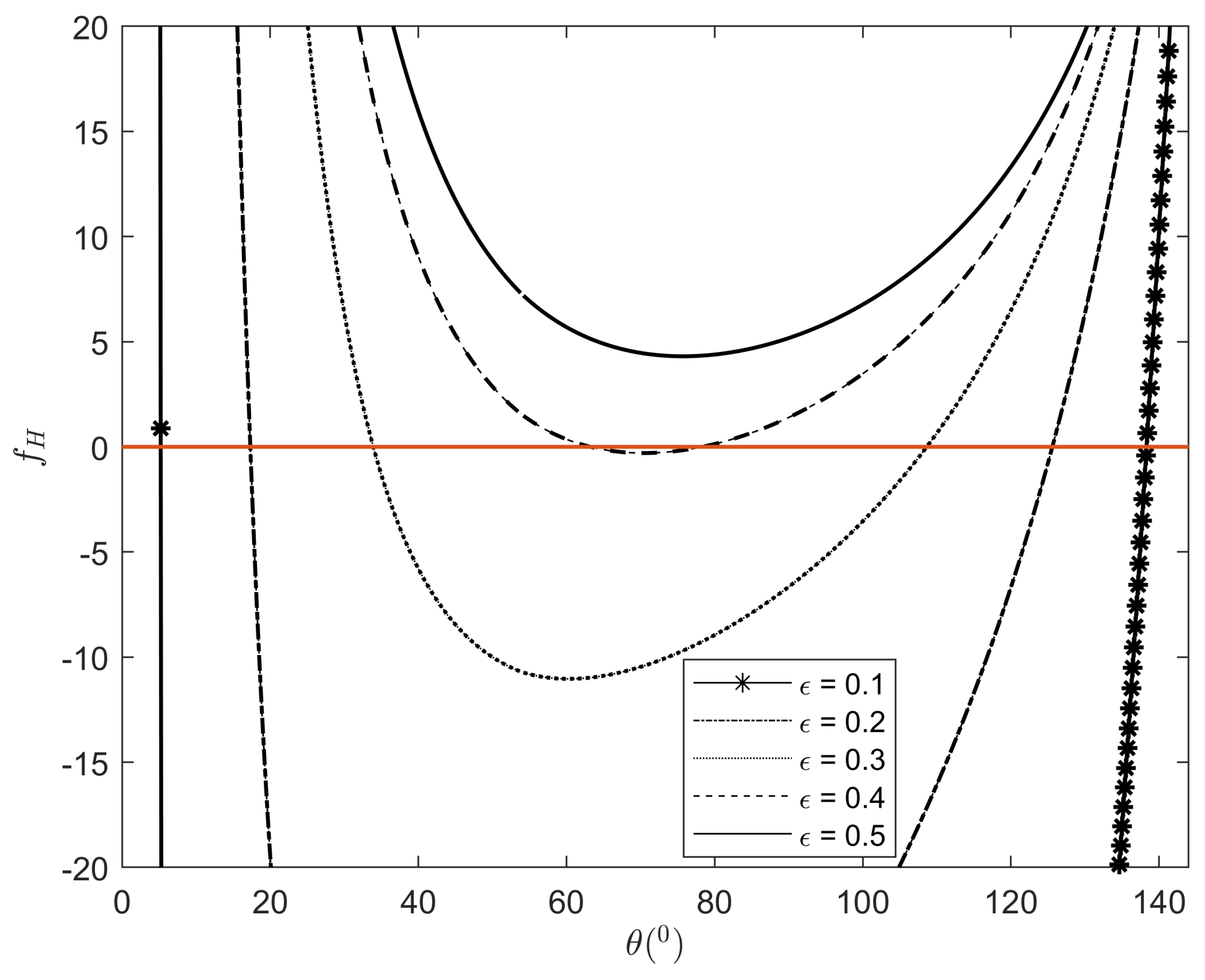
The particle can maintain its position at the free interface when $f_H=0$. Figure 2 demonstrates the existence of two steady-state equilibrium configurations as a function of $ϵ$ for a fixed contact angle and density ratio, where $D=2,10$ and $\alpha =0.2\pi$ represents a hydrophilic case and $\alpha =0.8\pi$ represents a hydrophobic case. The figures reveal two steady interface configurations at a small $ϵ$, but no solutions exist for a large $ϵ$. This occurs because increasing $ϵ$ allows a particle to be more easily pulled off the interface due to the net body force exceeding the capillary force. The stability of each steady interface configuration will be examined in the next section. For a hydrophobic particle ($\alpha =0.8\pi$), the probability of flotation is much larger. This phenomenon will be analyzed in detail in Section 3.

2.3. Stability Analysis of Steady Configuration

From Figure 2, we observe that two solutions exist, satisfying the condition of $f_H=0$. To distinguish between stable and unstable steady solutions, we examine small displacements in the vertical direction y for each equilibrium solution. With $y=H_0-cos\theta$ and $y^{*}=H_0^{*}-cos{\theta }^{*}$, where the superscript ∗ denotes evaluation at a small displacement of $\theta +\delta \theta$, the unbalanced force acting on the particle becomes

$$\begin{array}{c}\hfill F_t^{*}={\displaystyle \frac{2}{{ϵ}^2}}sin{\beta }^{*}sin{\theta }^{*}+{\displaystyle \frac{1}{3}}(2+3cos{\theta }^{*}-{cos}^3{\theta }^{*})-H_0^{*}{sin}^2{\theta }^{*}-{\displaystyle \frac{4}{3}}D.\end{array}$$

(44)

We define the net unbalanced force $\delta F$ as $F_t^{*}-F_t$. The system achieves stability when $\delta F$ becomes positive for any negative displacement or negative for any positive displacement, i.e., $\delta F/\delta y\le 0$, as the net force opposes the displacement. Therefore, stable configurations are characterized by negative values of $\delta F/\delta y$.

The net unbalanced force can be expressed as a truncated series in $\delta \theta$:

$$\begin{array}{c}\hfill \delta F={\displaystyle \frac{2}{{ϵ}^2}}\left(sin\beta cos\theta +sin\theta {\displaystyle \frac{dsin\beta }{d\theta }}\right)\delta \theta +sin\theta (-1+3{cos}^2\theta )\delta \theta -sin\theta (2H_{0}cos\theta -{sin}^2\theta )\delta \theta +{\left(\delta \theta \right)}^2.\end{array}$$

(45)

Since $\delta y=sin\theta \delta \theta$, $\delta F/\delta y$ takes the form

$$\begin{array}{c}\hfill \begin{array}{c}\hfill {\displaystyle \frac{\delta F}{\delta y}}={\displaystyle \frac{1}{sin\theta }}{\displaystyle \frac{\delta F}{\delta \theta }}={\displaystyle \frac{2}{{ϵ}^2}}\left({\displaystyle \frac{sin\beta }{tan\theta }}-cos\beta \right)+2cos\theta (cos\theta -H_0)\le 0.\end{array}\end{array}$$

(46)

Figure 3 and

Table 1. Values satisfying of $f_H=0$ with different values of $ϵ$, where $D=10$ and $\alpha =0.8\pi$.

	$\mathit{ϵ}=0.1$		$\mathit{ϵ}=0.2$		$\mathit{ϵ}=0.3$		$\mathit{ϵ}=0.4$
$\theta (°)$	$5.2$	$138.3$	$17.3$	$125.6$	$33.9$	$108.6$	$63.2$	$78.1$
$|H_0|$	$0.2968$	$0.1882$	$0.7573$	$0.5228$	$1.2211$	$0.8813$	$1.5464$	$1.3717$
${\displaystyle \frac{\partial F}{\partial y}}$	$1600.6$	$-220.5$	$161.9$	$-58.7$	$42.1$	$-22.8$	$6.04$	$-2.05$

demonstrate the existence of two steady-state particle–interface configurations as a function of $ϵ$, for $D=10$ and $\alpha =0.8\pi$. The results indicate that two steady interface configurations exist only below ${ϵ}_{max}$, beyond which no steady configurations exist. In this case, ${ϵ}_{max}$ lies between $0.4$ and $0.5$. For particles with a large $ϵ$, the magnitude of the net buoyancy force can exceed that of the capillary force.

The stability analysis reveals that the steady interface shape with negative $\delta F/\delta y$ values (Table 1) represents the stable configuration. The function $f_H$ provides crucial information about the maximum values of ${ϵ}_{max}$ and $D_{max}$. This investigation focuses on the steady particle–interface shapes characterized by negative values of $\delta F/\delta y$. The limitations in Lee’s previous work [27] stemmed from two factors: the computation of unstable solutions due to the improper selection of initial values in the numerical analysis, and the inability to verify the existence of dual solutions through differential equation methods.

2.4. Numerical Solution

In this section, we describe the numerical implementation method used to validate the asymptotic solutions. We introduce the parameter $\psi$ as the angle of meniscus inclination, defined by the relation $dy/dx=tan\psi$. Using this parameterization, Equation (1) can be decomposed into two ordinary differential equations:

$$\begin{array}{c}\hfill {\displaystyle \frac{dy}{d\psi }}={\displaystyle \frac{sin\psi }{Q^{*}}},{\displaystyle \frac{dx}{d\psi }}={\displaystyle \frac{cos\psi }{Q^{*}}}\end{array}$$

(47)

where $Q^{*}$ is given by

$$\begin{array}{c}\hfill Q^{*}={\displaystyle \frac{y}{l_c^2}}-{\displaystyle \frac{sin\psi }{x}}.\end{array}$$

(48)

Detailed derivations can be found in [27,34].

Applying the non-dimensionalization $Y=y/r_0$ and $X=x/r_0$ yields

$$\begin{array}{c}\hfill {\displaystyle \frac{dY}{d\psi }}={\displaystyle \frac{sin\psi }{Q}},{\displaystyle \frac{dX}{d\psi }}={\displaystyle \frac{cos\psi }{Q}}\mathrm{w}\mathrm{i}\mathrm{t}\mathrm{h}Q=BoY-{\displaystyle \frac{sin\psi }{X}}.\end{array}$$

(49)

Here, $Bo$ is the Bond number, which is equivalent to ${ϵ}^2$ discussed in the previous section. At the three-phase contact point $(X,Y)$ where $\psi =\beta$, the boundary condition Equation (2) becomes

$$\begin{array}{c}\hfill Y\left(\beta \right)=H_0,X\left(\beta \right)=sin\theta .\end{array}$$

(50)

The far-field boundary condition as $\psi$ approaches zero is

$$\begin{array}{c}\hfill Y\to 0,X\to \infty .\end{array}$$

(51)

Following [27], we obtain numerical solutions using Chebyshev nodes for the discretization of $\psi$. The calculations for X and Y proceed iteratively until the value of $\left|Y\right|$ at the last Chebyshev node falls below the tolerance of ${10}^{-3}$. The position of the contact line $H_0$ is determined relative to the unbounded flat interface, which is zero in the vertical direction. This approach of transforming the nonlinear equation into two ordinary differential equations parameterized by the inclination angle and discretization using Chebyshev nodes provides enhanced resolution near the triple contact points and at the infinity boundary [27]. This numerical solution was validated against Singh’s experimental data [22], showing agreement within 10% for different cases [27].

3. Results

We begin by comparing three different approaches: the matched asymptotic expansion, our numerical solution, and the classical numerical results of [18], as shown in

Table 2. Comparison of accuracy. Here, $D=6.266$, $r_0=1 \mathrm{mm}$, $ϵ=0.3703$, and $\alpha =\pi /2$ [18].

	$\mathit{\theta }$	$|{\mathit{H}}_0|$	$|{\mathit{y}}_{1000}|$ *
Huh and Scriven [18]	$54.5°$	0.73
Numerical solution, Equation (49)	$56.6°$	0.7022
f, Equation (29)	$56.6°$	0.7010
$\widehat{f}$, Equation (38)	$56.6°$	0.7030	0.0942
* $|y_{1000}|$ is the normalized depth at $x/r_0=1000$.

. The comparison uses the following parameters: the density ratio $D=6.266$, particle radius $r_0=1$ mm, $ϵ=0.3703$, and contact angle $\alpha =\pi /2$. The matched asymptotic solutions from Equation (29) and Equation (38) show excellent agreement with the numerical results from Equation (49) for both the filling angle, $\theta$, and the depth from the unbounded free surface, $|H_0|$, despite showing small differences from the numerical results of [18]. Here, $|y_{1000}|$ represents the normalized depth at $x/r_0=1000$, which will be discussed in detail later.

To further evaluate the accuracy of the matched asymptotic expansion, we calculated the filling angle $\theta$ and the depth $|H_0|$ for different values of $ϵ$ while maintaining fixed conditions of $D=10$ and $\alpha =0.8\pi$. These results are summarized in

Table 3. $f_H$ with different values of $ϵ$, where $D=10$ and $\alpha =0.8\pi$.

		$\mathit{ϵ}=0.05$	$\mathit{ϵ}=0.1$	$\mathit{ϵ}=0.2$	$\mathit{ϵ}=0.3$	$\mathit{ϵ}=0.4$
$\theta$	Numerical solution, Equation (49)	$142.4°$	$138.3°$	$125.6°$	$108.6°$	$78.4°$
	Asymptotic solution, Equation (42)	$142.4°$	$138.3°$	$125.6°$	$108.6°$	$78.1°$
$|H_0|$	Numerical solution, Equation (43)	$0.0600$	$0.1882$	$0.5229$	$0.8817$	$1.3717$
	f, Equation (29)	$0.0600$	$0.1882$	$0.5226$	$0.8795$	$1.3669$
	$\widehat{f}$, Equation (38)	$0.0600$	$0.1882$	$0.5228$	$0.8813$	$1.3717$
	$|y_{1000}|$	0	$0.0000114$	$0.0037274$	$0.0967$	$0.8282$

.

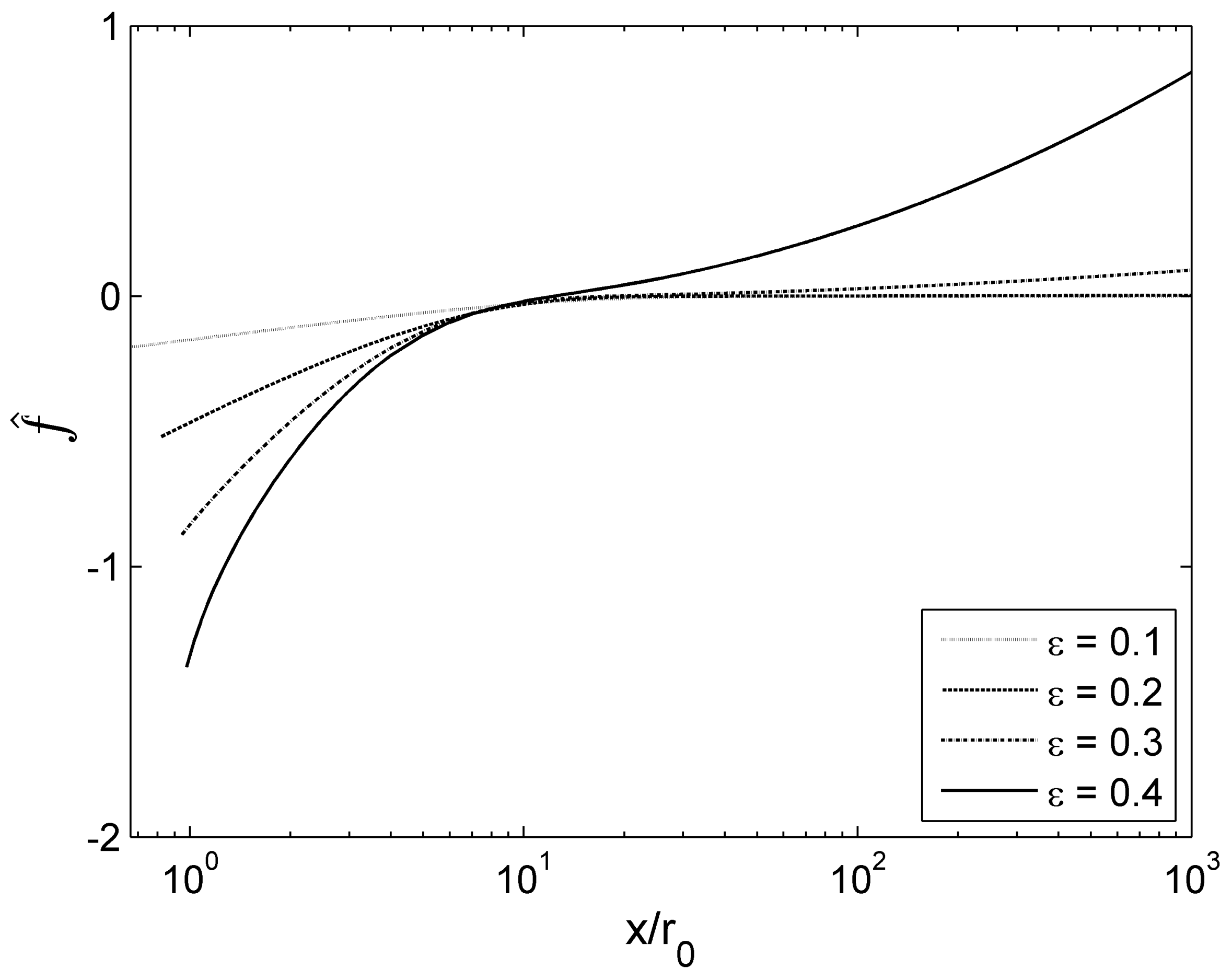
Figure 4 illustrates the matched asymptotic solution $\widehat{f}$ for different values of $ϵ$. The results demonstrate that the matched asymptotic solution maintains good accuracy across all values of $ϵ$. While Figure 4 reveals some discrepancies far from the particle for moderate $ϵ$ values, the solution provides excellent predictions for the filling angle $\theta$ and the depth $|H_0|$ near the particle, even at moderate $ϵ$ values.

To check the difference between the inner solution f and the composite solution $\widehat{f}$, Equation (38) can be expressed as

$$\begin{array}{c}\hfill \begin{array}{cc}\hfill \widehat{f}\left(z\right)-f\left(z\right)& =c(ln2-lnϵ-\gamma -lnz-K_0\left(ϵz\right))+{ϵ}^2\mathrm{terms}.\hfill \end{array}\end{array}$$

(52)

Therefore, near the particle at a small $ϵ$, the difference reduces to only ${ϵ}^2$ terms, resulting in quite small values. Although the ${ϵ}^2$ terms contain components of z, $z^2$, $lnz$, and ${ln}^{2}z$, their effect is negligible at a small $ϵ$.

To examine the difference far from the particle, Equation (38) can be rewritten as

$$\begin{array}{c}\hfill \begin{array}{cc}\hfill \widehat{f}\left(z\right)-F\left(ϵz\right)& =c(-ln2-lnz+ln(z+\sqrt{z^2-c^2})+{\displaystyle \frac{c^3}{4z^2}}+{ϵ}^2\mathrm{terms}.\hfill \end{array}\end{array}$$

(53)

As z approaches infinity, the difference is again limited to only ${ϵ}^2$ terms. However, unlike the near-particle case, the effect of the ${ϵ}^2$ terms becomes significant. This occurs because z, $z^2$, $lnz$, and ${ln}^{2}z$ exhibit divergent behavior at infinity. Consequently, the graph with $ϵ=0.4$ in Figure 4 shows divergence at a large z. However, no divergence occurs in $\widehat{f}$ for a sufficiently small $ϵ$. When focusing on the filling angle and depth induced by a submerged particle, the matched asymptotic expansion provides satisfactory solutions even at a large $ϵ$, as shown in Table 3. This accuracy is maintained because $\theta$ and $|H_0|$ are determined at the contact line on the particle, not far from the particle.

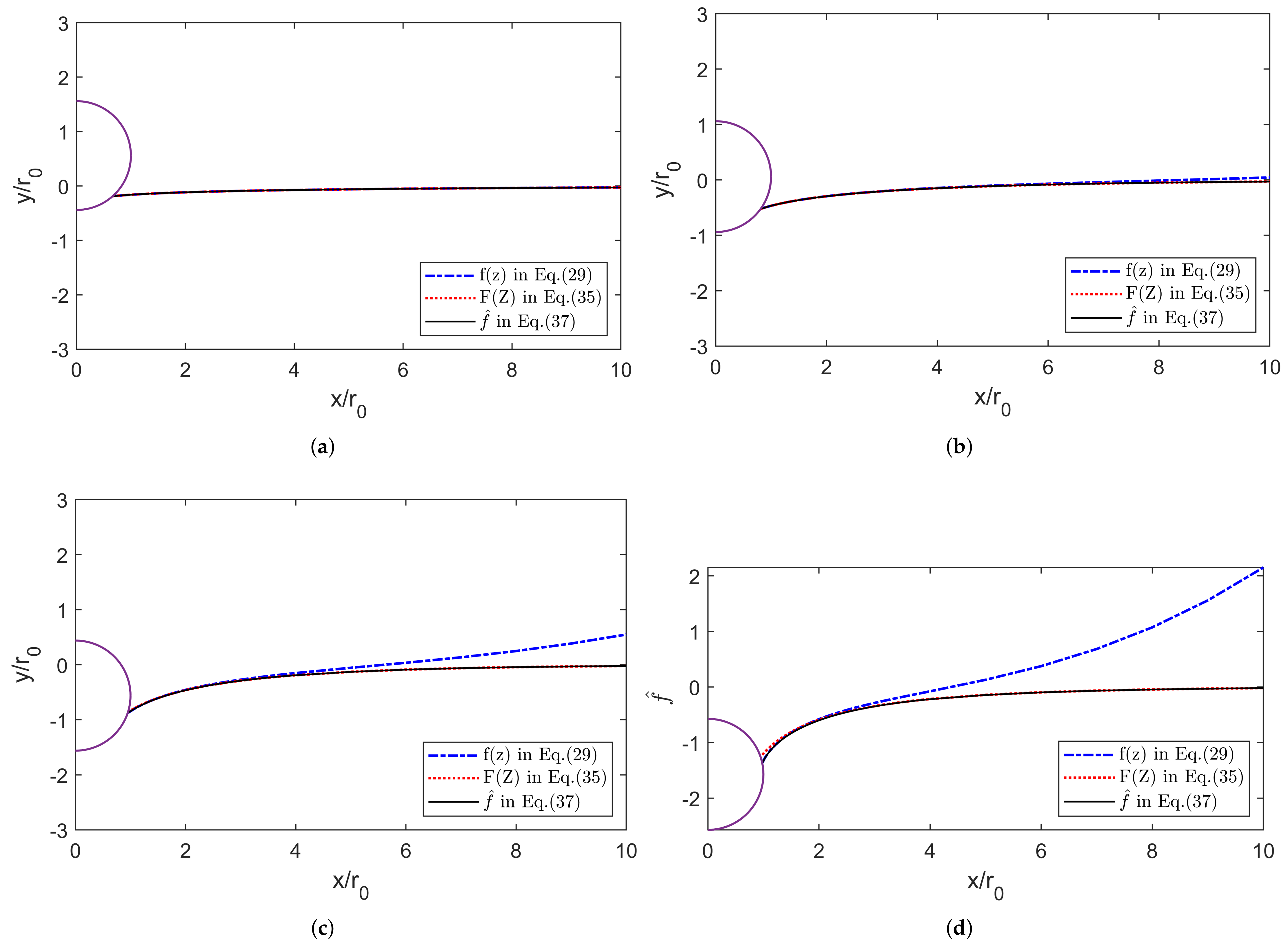
Figure 5 presents the inner (f), outer (F), and composite ($\widehat{f}$) asymptotic solutions with $D=10$ and $\alpha =0.8\pi$. The inner solution f agrees with the composite solution $\widehat{f}$ near the particle; however, it diverges as z approaches infinity for a large $ϵ$, as shown by the dash-dotted line. The outer solution (dashed line) demonstrates excellent agreement with the composite solution in all regions, including at the unbounded free surface. For all cases, the asymptotic solution $\widehat{f}$ within $x/r_0<10$ approaches the unbounded free surface $y=0$ asymptotically.

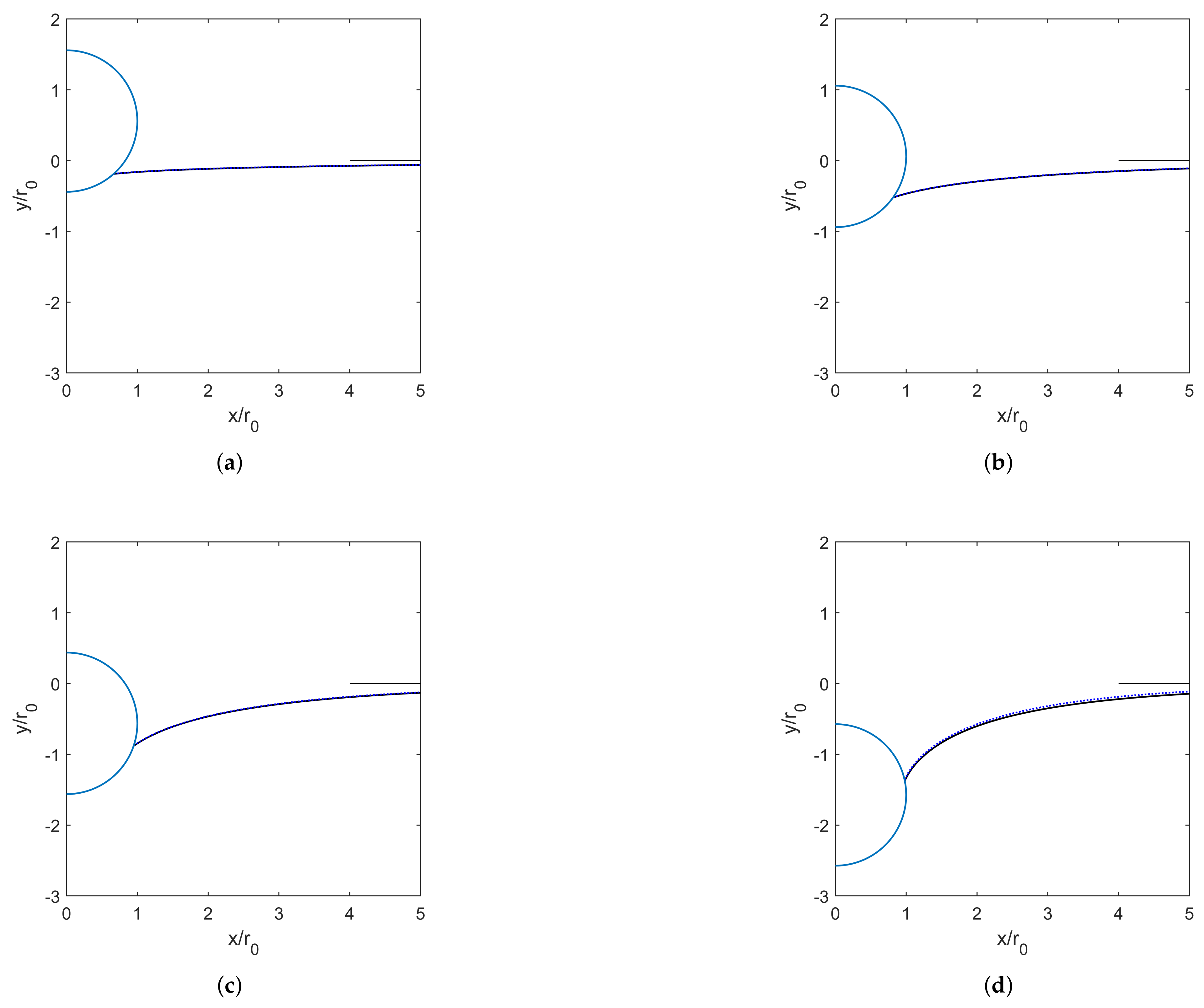
Figure 6 illustrates the surface trajectory deformed by a solid particle under the same conditions as Figure 5. The asymptotic solutions $\widehat{f}$ for different $ϵ$ values are compared with numerical results (represented by the dashed line). As $ϵ$ increases, the interface exhibits stronger curvature near the particle, and the depression depth of the submerged particle increases. Within the region $x/r_0<5$, both equilibrium configurations show excellent agreement. These results demonstrate that the matched asymptotic solutions accurately predict the equilibrium particle–interface configuration for a floating particle.

By comparing numerical and analytical methods, we observed that the particle radius to capillary length ratio ($ϵ$) significantly affects stability. Smaller values of $ϵ$ favor stability at the interface, while larger values may cause the particle to detach. Additionally, the contact angle ($\alpha$) impacts buoyancy behavior, particularly for hydrophobic particles ($\alpha$ close to 0.8$\pi$), which are more likely to float compared to hydrophilic particles ($\alpha$ close to 0.2$\pi$).

4. Conclusions

This study successfully analyzed the meniscus around a floating particle using matched asymptotic expansions and provided accurate analytical solutions. The results reveal two steady-state interface configurations, with one identified as stable through vertical stability analysis. Even for larger $ϵ$ values, the asymptotic solutions accurately predict the filling angle and the position of the three-phase contact line. Future research could explore buoyancy for particles of various shapes and investigate the buoyancy stability under dynamic conditions.

References

1. Nutt, C.W. Froth flotation: The adhesion of solid particles to flat interfaces and bubbles. Chem. Eng. Sci. 1960, 12, 133–141. [Google Scholar] [CrossRef]
2. Scheludko, A.B.; Teshev, B.V.; Bojadjiev, D.T. Attachment of particles to a liquid surface (Capillary theory of flotation). J. Chem. Soc. Faraday Trans. 1976, 72, 2815–2828. [Google Scholar] [CrossRef]
3. Hoseinian, F.; Rezai, B.; Kowsari, E.; Safari, M. Effect of impeller speed on the Ni(II) ion flotation. Geosystem. Eng. 2018, 22, 161–168. [Google Scholar] [CrossRef]
4. Carelse, C.; Manuel, M.; Chetty, D.; Taguta, J.; Safari, M.; Youlton, K. The flotation behaviour of liberated Platinum Group minerals in Platreef ore under reduced reagent conditions. Miner. Eng. 2022, 190, 107913. [Google Scholar] [CrossRef]
5. Pyke, B.; Farnasiero, D.; Ralston, J. Bubble particle heterocoagulation under trubulent conditions. J. Colloid Inter. Sci. 2003, 265, 141–151. [Google Scholar] [CrossRef]
6. Safari, M.; Hoseinian, F.; Deglon, D.; Filho, L.; Pinto, T. Impact of flotation operational parameters on the optimization of fine and coarse Itabirite iron ore beneficiation. Power Technol. 2022, 408, 117772. [Google Scholar] [CrossRef]
7. Verrelli, D.; Bruckard, W.J.; Koh, P.T.; Schwarz, M.P.; Follink, B. Particle shape effects in floatation. Part 1: Mircroscale experimental observations. Min. Eng. 2014, 58, 80–89. [Google Scholar] [CrossRef]
8. Crawford, R.; Ralston, J. The influence of particle size and contact angle in mineral flotation. Int. J. Min. Proc. 1988, 23, 1–24. [Google Scholar] [CrossRef]
9. Fang, J.; Ge, Y.; Yu, J. Effects of particle size and wettability on froth stability in a collophane flotation system. Powder Technol. 2021, 379, 576–584. [Google Scholar] [CrossRef]
10. Guzman, E.; Ortega, F.; Rubio, R.G. Forces controlling the assembly of particles at fluid interfaces. Langmuir 2022, 38, 13313–13321. [Google Scholar] [CrossRef]
11. Ma, X.; Nguyen, N.; Nguyen, A. A review on quantifying the influence of lateral capillary interaction on the particle floatability and stability of particle-laden interfaces. Adv. Colloid Int. Sci. 2022, 307, 102731. [Google Scholar] [CrossRef] [PubMed]
12. Gao, Y.X. A thermodynamic limitation of the maximum speed of wetting of a solid surface by a liquid. Appl. Phys. Let. 2003, 83, 4447–4449. [Google Scholar] [CrossRef]
13. Liu, D.; Evans, G.; He, Q. Critical fall height for particle capture in film flotation: Importance of three phase contact line velocity and dynamic contact angle. Chem. Eng. Res. Des. 2016, 114, 52–59. [Google Scholar] [CrossRef]
14. Li, A.; Li, H.; Zhao, Z.; Xue, L.; Li, Z.; Li, K.; Li, M.; Song, Y. Adjustable object floating states based on three-segment three-phase contact line evolution. Proc. Nat. Acad. Sci. USA 2022, 119, e2201665119. [Google Scholar] [CrossRef]
15. Extrand, C.W.; Moon, S. Using the flotation of a single sphere to measure and model capillary forces. Langmuir 2009, 25, 6239–6244. [Google Scholar] [CrossRef]
16. Liu, X.; Wang, X.; Liang, Y.; Zhou, F. Floating behavior of hydrophobic glass spheres. J. Colloid Int. Sci. 2009, 336, 743–749. [Google Scholar] [CrossRef]
17. Cooray, H.; Cicuta, P.; Vella, D. Floating and sinking of a pair of spheres at a liquid-fluid interface. Langmuir 2017, 33, 1427–1436. [Google Scholar] [CrossRef]
18. Huh, C.; Scriven, L.E. Shapes of axisymmetric fluid interfaces of unbounded extent. J. Colloid Int. Sci. 1969, 30, 323–337. [Google Scholar] [CrossRef]
19. Huh, C.; Mason, S.G. The flotation of axisymmetric particles at horizontal liquid interfaces. J. Colloid Int. Sci. 1974, 47, 271–289. [Google Scholar] [CrossRef]
20. Rapacchietta, A.V.; Neumann, A.W. Force and free-energy analyses of small particles at fluid interfaces, II. spheres. J. Colloid Int. Sci. 1977, 59, 555–567. [Google Scholar] [CrossRef]
21. Stoos, J.A.; Leal, L.G. A spherical particle straddling a fluid/gas interface in an axisymmetric straining flow. J. Fluid Mech. 1990, 217, 263–298. [Google Scholar] [CrossRef]
22. Singh, P.; Joseph, D.D. Fluid dynamics of floating particles. J. Fluid Mech. 2005, 530, 31–80. [Google Scholar] [CrossRef]
23. Feng, D.; Nguyen, A.V. A novel quantitative analysis of the local deformation on the air-water surface by a floating sphere. Colloids Surf. A 2016, 504, 407–413. [Google Scholar] [CrossRef]
24. Deryagin, B.V. Theory of the distortion of a plane surface of a liquid by small objects and its application to the measurement of the contact angle of thin filaments and fibers. CR Acad. Sci. URSS 1946, 51, 519–522. [Google Scholar]
25. Princen, H.M. The equilibrium shape of interfaces, drops, and bubbles. Rigid and deformable particles at interfaces. Surf. Colloid Sci. 1969, 2, 1–84. [Google Scholar]
26. Vella, D.; Lee, D.; Kim, H.Y. The load supported by small floating objects. Langmuir 2006, 22, 5979–5981. [Google Scholar] [CrossRef]
27. Lee, J. The static profile for a floating particle. Colloids Interfaces 2018, 2, 18. [Google Scholar] [CrossRef]
28. James, D.F. The meniscus on the outside of a small circular cylinder. J. Fluid Mech. 1974, 63, 657–664. [Google Scholar] [CrossRef]
29. Lo, L.L. The meniscus on a needle—A lesson in matching. J. Fluid Mech. 1983, 132, 65–78. [Google Scholar] [CrossRef]
30. Proudman, I.; Pearson, J.R.A. Expansions at small Reynolds numbers for the flow past a sphere and a circular cylinder. J. Fluid Mech. 1957, 2, 237–262. [Google Scholar] [CrossRef]
31. Van Dyke, M. Perturbation Methods in Fluid Mechanics; Academic Press: Cambridge, MA, USA, 1964. [Google Scholar]
32. Hinch, E.J. Perturbation Methods; Cambridge University Press: Cambridge, UK, 1991. [Google Scholar]
33. Fraenkel, L.E. On the method of matched asymptotic expansions, part I: A matching principle. Proc. Camb. Phil. Soc. 1969, 65, 209–231. [Google Scholar] [CrossRef]
34. Pozrikidis, C. Introduction to Theoretical and Computational Fluid Dynamics; Oxford University Press: Oxford, UK, 1997. [Google Scholar]
Figure 1. Physical configuration of a floating sphere.
Chemengineering 09 00028 g001
Figure 2. Behavior of f H with D = 2 , 10 and α = 0.2 π , 0.8 π . (a) α = 0.2 π and D = 2; (b) α = 0.8 π and D = 2; (c) α = 0.2 π and D = 10; (d) α = 0.8 π and D = 10.
Chemengineering 09 00028 g002
Figure 3. f ^ with different values of ϵ , where D = 10 and α = 0.8 π .
Chemengineering 09 00028 g003
Figure 4. f ^ with different values of ϵ , where D = 10 and α = 0.8 π .
Chemengineering 09 00028 g004
Figure 5. Illustration of asymptotic solutions with D = 10 and α = 0.8 π . (a) ϵ = 0.1; (b) ϵ = 0.2; (c) ϵ = 0.3; (d) ϵ = 0.4.
Chemengineering 09 00028 g005
Figure 6. Agreement between asymptotic solutions, f ^ , and numerical results, where D = 10 and α = 0.8 π . (a) ϵ = 0.1; (b) ϵ = 0.2; (c) ϵ = 0.3; (d) ϵ = 0.4.
Chemengineering 09 00028 g006