Abstract
The improvement in energy efficiency is recognized as one of the significant parameters for achieving our net-zero emissions target by 2050. One exciting area for development is conventional carbon capture technologies. Current amine absorption-based systems for carbon capture operate at suboptimal conditions resulting in an efficiency loss, causing a high operational expenditure. Knowledge of qualitative and quantitative speciation of CO2-loaded alkanolamine systems and their interactions can improve the equipment design and define optimal operating conditions. This work investigates the potential of Raman spectroscopy as an in situ monitoring tool for determining chemical species concentration in the CO2-loaded aqueous monoethanolamine (MEA) solutions. Experimental information on chemical speciation and vapour-liquid equilibrium was collected at a range of process parameters. Then, partial least squares (PLS) regression and an artificial neural network (ANN) were applied separately to develop two Raman species calibration models where the Kent–Eisenberg model correlated the species concentrations. The data were paired and randomly distributed into calibration and test datasets. A quantitative analysis based on the coefficient of determination (R2) and root mean squared error (RMSE) was performed to select the optimal model parameters for the PLS and ANN approach. The R2 values of above 0.90 are observed for both cases indicating that both regression techniques can satisfactorily predict species concentration. ANN models are slightly more accurate than PLS. However, PLS (being a white box model) allows the analysis of spectral variables using a weight plot.
1. Introduction
Carbon dioxide (CO2) is deemed a global environmental concern due to its role in global warming and climate change as a greenhouse gas [1,2]. Industrial activities such as oil and gas processing, power generation and steel and iron production contribute 64% of total CO2 emissions [3,4]. In the natural gas production industry, CO2 had been among the main contaminants that need to be removed. In addition to environmental concern, CO2 is also corrosive to natural gas transmission pipelines with the presence of water leading to the formation of carbonic acid, posing a major safety risk and thus requiring stringent regulation and maintenance to be implemented during operation to manage it [5]. The gross heating value of sales gas is also affected with sale price per volume decreases as CO2 volume increases [6]. As more low-CO2 gas fields deplete rapidly and the demand for cleaner energy increases, the need to monetize the high-CO2 containing natural gas fields increases.
Chemical absorption of CO2 from gas streams using aqueous amine solvent is considered to be a robust separation technology that had found commercial prevalence in the natural gas processing industry and will remain relevant for years to come [7]. Amine absorption is feasible for CO2 removal due to its technology maturity, operational robustness and process flexibility. Amine absorption technology also has relatively fast absorption rate and higher capacity compared to other CO2 removal technologies [8]. Amine reacts with CO2 through acid-base reaction to form ionic species as well as carbamate in primary and secondary amines due to its basic nature [9]. Due to the plateau growth trends in the development of other CO2 removal technologies as well as more stringent regulation for CO2 emission around the globe, it can be predicted that the total application of amine solvent for CO2 removal applications will continue to grow.
Monoethanolamine (MEA) is an industrial benchmark for CO2 removal applications and a widely used amine in the industry [10]. Compared to secondary and tertiary amine, the higher reaction rate of MEA with CO2 proves to be the main advantages of its selection in CO2 removal applications [11]. MEA is also capable of reducing CO2 content in a gas stream to a trace level [9].
Increasing the efficiency of an MEA process for CO2 removal depends considerably upon the understanding of the thermodynamics and kinetics of the system. This could not be properly established unless all the species of the system and their interactions are well known and understood through constant observation and analysis of the system itself. Raman spectroscopy is an analytical technique that is applicable for quantitative analysis of chemical species in a system. Understanding that a Raman spectrum from a CO2-loaded aqueous MEA system uniquely characterizes the chemical species present in the system. The information can be utilized for gaining an understanding of the dynamics and kinetics of the system towards optimizing the process [12]. Raman spectroscopy is non-destructive and non-invasive for analysing liquid or gas system as well as capable to analyse wide range of physical state. The technique had been utilized to quantify phase equilibria, transport properties and species’ concentration in liquid and gas sample [13,14,15]. Raman spectroscopy possesses lower water absorptivity compared to Fourier Transform Infrared (FT-IR) technique resulting in less distortion for aqueous system application [15,16].
Raman spectra carry information regarding the chemical species within the monitored system. The information was contained within a specific range of variable within the Raman spectrum which was defined as a characteristic band. The peak (which was contained within the characteristic bands) was formed due to the inelastic Raman scattering as a result of the collision between ions or molecules with the laser beam. The characteristic bands are unique for each chemical species in the CO2-loaded MEA system. The observed peak changes within the characteristic bands are proportional to the changes in the respective species’ concentration in accordance with Beer-Lambert’s Law [17].
Interpreting the spectrum from Raman spectroscopy requires the development of a calibration model specific to the chemical species of interest. The development of such a model requires data in the form of Raman spectra with the respective species concentration determined. The commonly applied method for acquiring species concentration data includes the wet chemistry method and application of the thermodynamic model. The wet chemistry method was the earliest technique to be utilized for quantifying species concentration in a system. It is often used due to the unavailability of an accurate thermodynamic model as well as the lack of required parameters to regress into thermodynamic models [18]. However, the method is prone to human errors due to dependency on personnel for properly conducting the laboratory work. In addition, there are also chemical species that are difficult to synthesize in the laboratory, thus preparing standard solution for the species is difficult [12] and requires a large number of man and machine hours for overall analysis [4,13].
Application of a thermodynamic model for CO2-loaded amine speciation analysis can minimize human errors and overall time required as well as provides means to estimate species concentration of chemical species which are difficult to synthesize. The Kent–Eisenberg model is a thermodynamic model developed for acid gases-loaded amine systems [19]. The model is well-known for its simplicity that is achieved by lumping all the non-idealities into the equilibrium constants which are then fitted to the experimental data, resulting in quick estimation while maintaining good correlative accuracy [20]. Other complex models use excess Gibbs energy or a combination of Equation of State and Gibbs energy approach, requiring a substantial number of regression parameters for iteration compared to the much simpler Kent–Eisenberg model [21]. The measurement accuracy of a modified version of the Kent–Eisenberg model was proven to be good within the range of 0.2 to 0.8 mol of CO2 per mol of amine [22,23,24].
Developing a Raman calibration model requires the application of a multivariate calibration technique. The requirement is due to the multivariate nature of the Raman spectrum. Each Raman spectrum is a linear combination of the pure compound spectra from chemical species in the system [12]. A Raman calibration model can be developed by first identifying the spectral peak of the species of interest. The spectral peak is identified by comparing the spectra with that from pure compound. The peak height or area of the identified spectra is then quantified against the measured species’ concentration [6]. For a complex system with various chemical species, multiple spectral peaks may overlap causing difficulties in identifying and measuring the respective peak area. Each variable within the Raman spectrum is also highly correlated to each other and needs to be uncorrelated before the species calibration model can be constructed. This requires the application of a dimensionality reduction technique.
Principal component analysis (PCA) is a dimensionality reduction technique that transforms the original variables into new, orthogonal variables called principal components. Each principal component is a linear combination of the original variables [25,26]. Construction of principal components maximizes the percentage of explained variance for the first component. The percentage subsequently reduced as additional principal components are added. Such a hierarchical structure is attained as principal components are constructed to be orthogonal to each other. The orthogonality and hierarchical structure of principal components allow relevant components with a high percentage of explained variance to be identified. The components can then be used for developing the Raman calibration model by applying a regression technique such as principal component regression (PCR) [27].
The concept of variable transformation towards orthogonality in PCA was well-integrated in the more advanced regression technique, called partial least squares (PLS) regression. The PLS regression model was developed using components that were constructed to maximize the correlation between predictor and response variables while also maximizing the explained variance within each predictor and response variables [28]. The approach in the PLS technique allows the construction of a simpler model compared to PCR. However, modelling a non-linear relationship using a linear regression technique such as PLS could impact accuracy. A non-linear relationship can exist in Raman spectral data due to overlapping signals, inconsistency in particle sizes within the sample, contaminants from external or ambient light and use of non-homogeneous or light-absorbing samples.
Modelling such a non-linear relationship might require the application of a non-linear regression technique. With the advancements made in the field of machine learning, the application of an artificial neural network (ANN) in chemometrics is also gaining traction [29]. ANN is a non-linear regression technique by virtue of utilizing a non-linear activation function. This capability can potentially improve measurement accuracy made by a process analyser compared to PCR and even PLS-based calibration model in real-world application [30,31,32].
Raman spectroscopy has been applied previously to quantify species concentration in a CO2-loaded aqueous MEA system. Souchon et al. studied species distribution in various amine types using Raman spectroscopy. Species concentration was derived from the reference solutions that were measured by a 13C nuclear-magnetic resonance (NMR) spectrometer. The work concluded that Raman spectroscopy can achieve lower analysis time compared to NMR due to the latter requires longer relaxation times per spectrum. The work also highlighted the importance of pairing a thermodynamic model with spectral measurement tools in estimating the quantities of carbamate ion, which are not measurable through the wet chemistry method [12]. Wong et al. investigated the chemical speciation in CO2-loaded aqueous MEA at varying pressure and temperature ranges using Raman spectroscopy. The author developed calibration models by manually plotting peak area ratio from the spectrum against species concentration, which was derived through the wet chemistry method. The models can predict species concentration with good accuracy [6]. Jinadasa et al. investigated the application of Raman spectroscopy for CO2-loaded, 30 wt% MEA solutions at room pressure and temperature. Using the PLS regression technique combined with offline titration analysis and Kent–Eisenberg thermodynamic models, the Raman calibration models are developed and the in situ monitoring technique was tested with good results [33,34]. Zubair et al. utilized Raman spectroscopy for measuring CO2 concentration in aqueous diethanolamine (DEA), methyldiethanolamine (MDEA) as well as a combination of both. The development of a calibration model in their work utilized PLS regression and a model was developed to include CO2 loading range above 0.5 for high-pressure applications [35]. Similarly, the author also investigated the application of Raman spectroscopy for monitoring species concentration in CO2-loaded aqueous DEA systems with a CO2 loading range of up to 0.98, utilizing the PLS regression technique for developing a calibration model [36]. It can be established that previous research work within the area focused mainly on the application of PLS regression methods, while other multivariate regression methods remained unexplored.
In this work, Raman species calibration models for CO2-loaded aqueous MEA system at 3, 4 and 5 molar MEA concentrations were developed using PLS regression and ANN. To develop the calibration models, Raman spectra of the system were first acquired using a vapour-liquid equilibrium (VLE) experimental setup with Raman spectroscopy installed. Next, CO2 loading values were calculated using a pressure drop method with ideal system assumed. The experimental VLE data together with CO2 loading were used on the regressed modified Kent–Eisenberg model to calculate the species concentration. The smoothed and centred Raman spectra together with the respective species concentration data were then utilized for developing the Raman calibration models using PLS regression and ANN techniques. Comparisons were made between the developed models based on the predictive performance by evaluating the coefficient of determination (R2) and root mean squared error (RMSE).
2. Materials and Methods
2.1. Materials
Materials required for conducting the VLE experiment are detailed in Table 1. Monoethanolamine was sourced from Merck Sdn. Bhd, while deionized water was obtained in-house. Carbon dioxide gas was procured from Linde Malaysia Sdn. Bhd.

Table 1.
Table of materials for the experiment.
Aqueous MEA solutions at 3, 4 and 5 molar strength were prepared by first weighing the required quantity of MEA on a Sartorius BSA2245S-BW mass balance. The weighted MEA was added to a 250 mL volumetric flask. Deionized water was added to the volumetric flask to prepare the solution at the required concentration. Each solution was prepared at a controlled temperature of 298.15 K.
2.2. Experimental Setup and Method
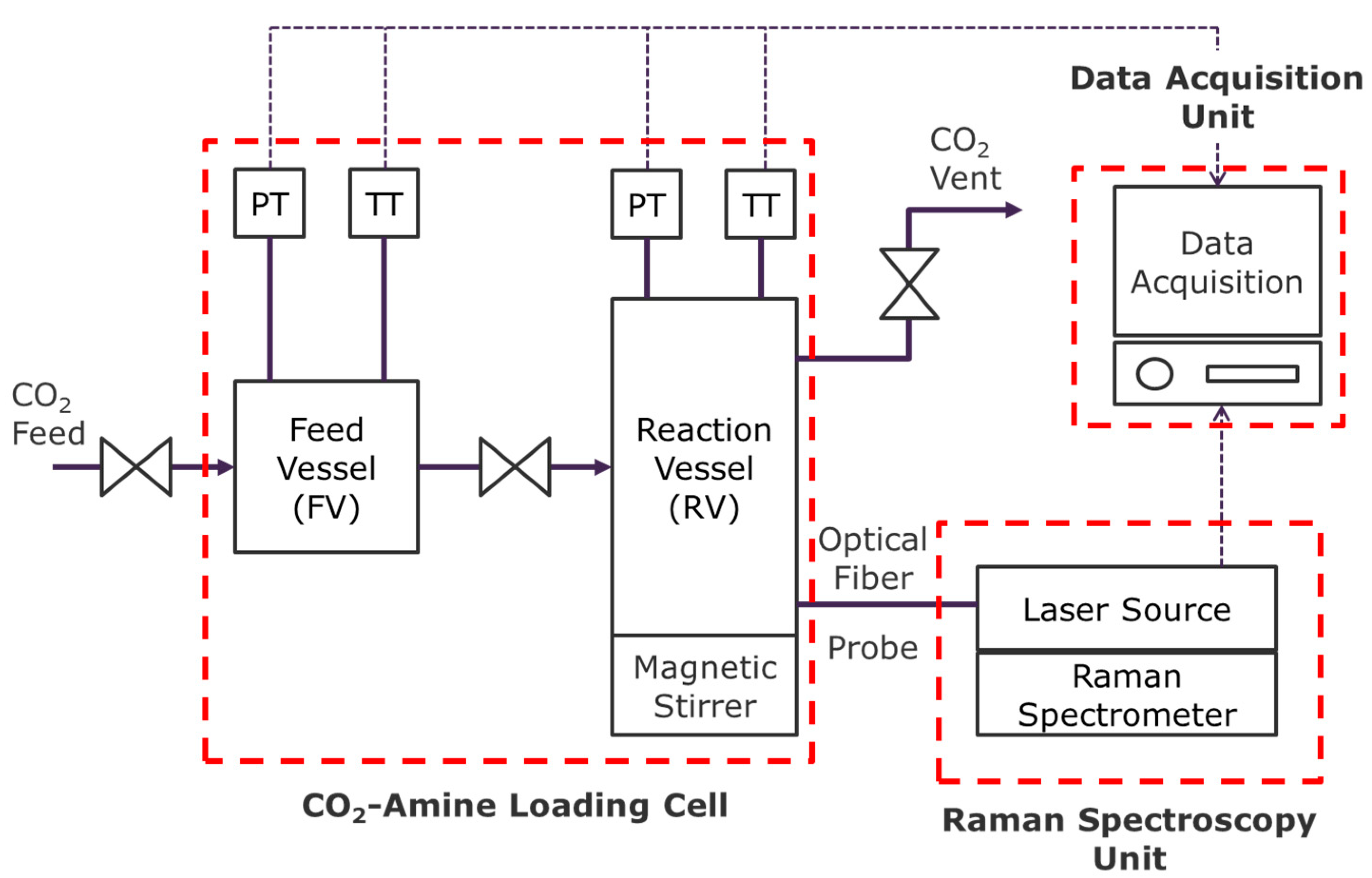
The VLE experimental setup was constructed as depicted in Figure 1. The setup consists of three sub-units which are CO2-amine loading cell, Raman spectroscopy unit and data acquisition unit. The CO2-amine loading cell consists of a 435 mL feed vessel connected to a 460 mL stainless steel reaction vessel. Both vessels are built with integrated pressure and temperature sensors to measure conditions and gathering experimental data. A CO2 feed line was connected to the feed vessel to supply CO2 gas into the experimental setup. A ceramic heater was installed around the reaction vessel to regulate system temperature. A CO2 vent line was installed at the top side of the reaction vessel to allow vessel degassing. A magnetic stirrer was used inside the reaction vessel throughout the experimental work to maintain mass transfer between the gas and liquid phase.

Figure 1.
Experimental setup to collect vapour-liquid equilibrium (VLE) data and Raman spectrum.
A Raman spectroscopy unit was procured from StellarNet. The unit consists of a Raman spectrometer and laser source. The Raman spectrometer has a resolution of 4 cm−1 with signal to noise ratio of 1000:1 while the laser source uses 500 W of power-producing laser beam with a wavelength of 785 nm. A probe connected to the Raman spectroscopy unit by an optical fibre cable was mounted at the side of the reaction vessel where a sapphire-glass window was built. The probe directed the laser beam towards the system and retrieved the resulting Raman scattering for the Raman spectrometer. The data acquisition unit was pre-installed with SpectraWiz software and serves to process the data received from the Raman spectroscopy unit.
In a typical run, the prepared aqueous MEA solution was firstly loaded into the reaction vessel. The temperature for each run was set at 303.15 K. CO2 gases were then introduced into the reaction vessel and the aqueous MEA solution was continuously stirred until an equilibrium state was reached. The temperature and pressure of the system were continuously recorded using built-in temperature and pressure transmitters throughout the experimental run for CO2 loading calculation using Equation (1) [15,35].
After the equilibrium state was reached, CO2 was further introduced into the reaction vessel and the process was repeated until the targeted CO2 loading in the aqueous MEA solution was reached inside the reaction vessel. The recorded Raman spectra were within the range of 0 to 2800 cm−1. Forty (40), 67 and 66 datapoints for the Raman spectra were gathered for 3, 4 and 5 molar aqueous MEA solutions, respectively.
2.3. Thermodynamic Framework and Kent–Eisenberg Model
The modified Kent–Eisenberg model was used to estimate the species concentration for the CO2-loaded aqueous MEA solutions in equilibrium [20]. The model is an improved version based on the work by Kent and Eisenberg [19]. Aqueous MEA reaction with CO2 follows an acid-base reaction and produced numerous ions. Equations (2)–(6) describe CO2 dissolution into MEA.
Dissociation of a protonated alkanolamine:
Reversion of carbamate to bicarbonate:
Hydrolysis and ionization of dissolved CO2:
Dissociation of bicarbonate:
Ionization of water:
Based on the defined chemical reactions, the equilibrium constants for each reaction are as follows:
The value for equilibrium constants K2, K3, K4 and K5 were calculated based on the work of Edwards et al. [37], whereas the value of K1 was treated as a fitting parameter to the experimental values. To fit the experimental loading data into the model, a parameter is defined where:
As for f:
The purpose of fitting the model with experimental loading data is so that accurate calculation of speciation data is acquired. The defined serve as an adjustable parameter to improve the prediction accuracy of the model towards the experiment parameters [6,20,38].
The unknowns were found by simultaneously solving the five reaction equations and three balance equations detailed below:
Amine balance:
CO2 balance:
Charge/electroneutrality balance:
Henry’s law is applied to quantify the concentration of carbon dioxide dissolved in the liquid phase:
The equations were solved in a polynomial form:
where:
Equation (18) was solved using MATLAB to find the roots. Five numerical values were obtained, in which one of them is the concentration of hydrogen ion. The valid hydrogen ion concentration is within the range of 10−7 to 10−12 molar with respect to the pH value of between 7 and 11 in the loaded and unloaded MEA solution [22]. The concentration of each chemical species was then calculated using Equations (7)–(11).
2.4. Calibration Models Development and Evaluation
The gathered Raman spectra and the species concentration estimated using the regressed modified Kent–Eisenberg model were paired and classified according to the total MEA concentration in the system from which the data originated. The classification of the dataset is presented in Table 2. Each dataset was then randomly divided into training and test datasets. The training dataset was used to develop a calibration model of the chemical species. The test dataset was then used to validate the performance of the developed calibration model externally, thus the test dataset was excluded from the model training. As for ANN, the training data were further divided randomly into a validation dataset which was used during model training to pre-validate model performance for early stopping implementation. Generally, 60% to 70% of the data were randomly assigned as training data while the remaining 30% to 40% were assigned as test data [39,40,41].

Table 2.
Table of materials for the experiment.
Before model development, Raman spectra were preprocessed through the application of Savitzky-Golay smoothing, followed by mean centring and scaling of the spectra. Savitzky-Golay smoothing was performed to reduce noise while preserving information contained in characteristic peaks within the spectrum. The application was through a built-in filter in MATLAB with smoothing degree and range of filter span adjustment dictates the smoothing effects on the individual spectrum. The optimal smoothing parameters were determined by observing the filter effects on the performance of the developed models. Mean centring was then performed on each Raman spectrum by subtracting the mean value of a variable from the respective variable in each observation in the MATLAB environment.
Raman calibration models were developed by applying PLS and ANN techniques on the preprocessed Raman spectra and the estimated species concentration, which served as a predictor and response data, respectively. While the form of response data used for model developments was similar for both techniques, the form of the predictor data differs between both techniques. For the PLS model, preprocessed Raman spectra were used directly while for ANN, the PCA score from the transformed Raman spectra was used. Full Raman spectrum range (160 to 2800 cm−1) were utilized for the model development.
PLS-based Raman species calibration models were developed using the PLSREGRESS function in MATLAB, which utilized the SIMPLS algorithm for fast iterations [28,42]. During the execution of the PLSREGRESS function, both Raman spectra and species concentration data were each transformed into a PLS component, which is a linear combination of each variable within the data. The PLS component was constructed such that the variance explained by the component as well as the correlation between the predictor and the response variables were maximized. Each of the constructed PLS components was also orthogonal to the others. The orthogonality resulted from the deflation step performed at the end of each component construction. The deflation step removes the variance explained by the current PLS component from the error matrix while preserving the unexplained variance. Additional PLS components were then constructed using the error matrix. Initial PLS-based models were developed using 15 components. Such a large number of components is to ensure that all-important information was considered for developing a calibration model for a particular response variable. Diagnostics from the developed model were then used to select an optimal number of components for the final model.
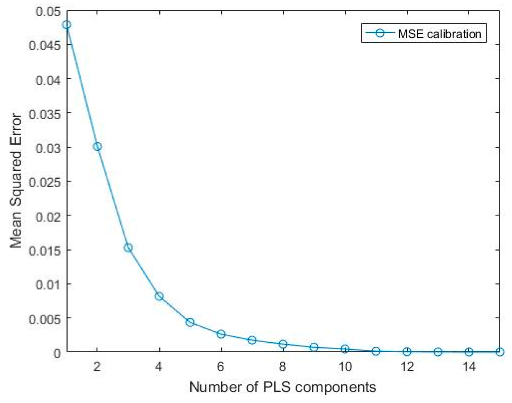
Application of the PLSREGRESS function on the dataset produces several outputs, which include the loadings and scores for the predictor and response data, the PLS regression coefficients, and a matrix containing the percentage of variance explained by the developed model. Using the percentage-explained variance data, a PLS variance plot (which is a plot of cumulative percent explained variance against the PLS component) was drawn. The PLS plot was used to estimate the potential number of PLS components to be used in developing the calibration model. These PLS components were determined up to the point where the variance profile flattened. Beyond that point, the components do not contain significant information towards the model and will lead to overfitting [27]. An example of a scree plot is depicted in Figure 2 revealing that mean squared error (MSE) reduced as the number of components increased. However, the plotted trend flattens after 6 components. The area before the 6th component was defined as scree region and was retained in the final model. A similar method was conducted in selecting the number of components for PLS-based calibration models.
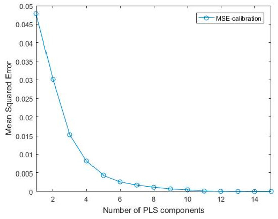
Figure 2.
Scree plot for partial least squares (PLS)-based CO2 loading Raman calibration model.
ANN-based Raman species calibration models were developed in MATLAB using the built-in Neural Network Toolbox combined with manual parameter adjustments. An untrained neural network architecture was initiated with three layers as default consisting of one input layer, one hidden layer and one output layer. A single hidden layer can act as a universal approximator capable of modelling any functions. Although there is a possibility of attaining quicker training time, additional hidden layers rarely improve the performance of calibration models versus using a single hidden layer [43,44,45].
For the input layer, raw Raman spectra were first compressed into principal components (PC) using principal component analysis (PCA). The score was then used as input for ANN. The step was implemented to reduce the dimension and extract only the relevant features from the data for lower memory requirement and faster iteration time [26,46,47]. The number of input nodes was set based on the number of principal components extracted using PCA. The number of output nodes was set to one to account for the respective chemical species concentration. Similar to the consideration made for PLS models, 15 LVs was selected for the initial training. The number is then further lowered during optimization. Additionally, the iterative optimization process on neural network structure during training will minimize the significance from less relevant input towards the resulting output [48]. One hidden layer was set for the initial design with one node to constraint model complexity and minimize overfitting. Additional nodes improve the prediction performance in the presence of slight non-linearity, which is common in multivariate datasets [48]. The number of nodes was subsequently adjusted based on the observed model performance. For the output layer, one node was used similar to the number of targeted outputs. The tan-sigmoid function was set as an activation function to allow flexibility for modelling non-linearity during training. MSE was implemented as the cost function to measure the performance and as a learning parameter for the optimization algorithm during ANN training. Random weights were assigned with the values constrained within −1 and 1 corresponding to the assigned activation function for the network.
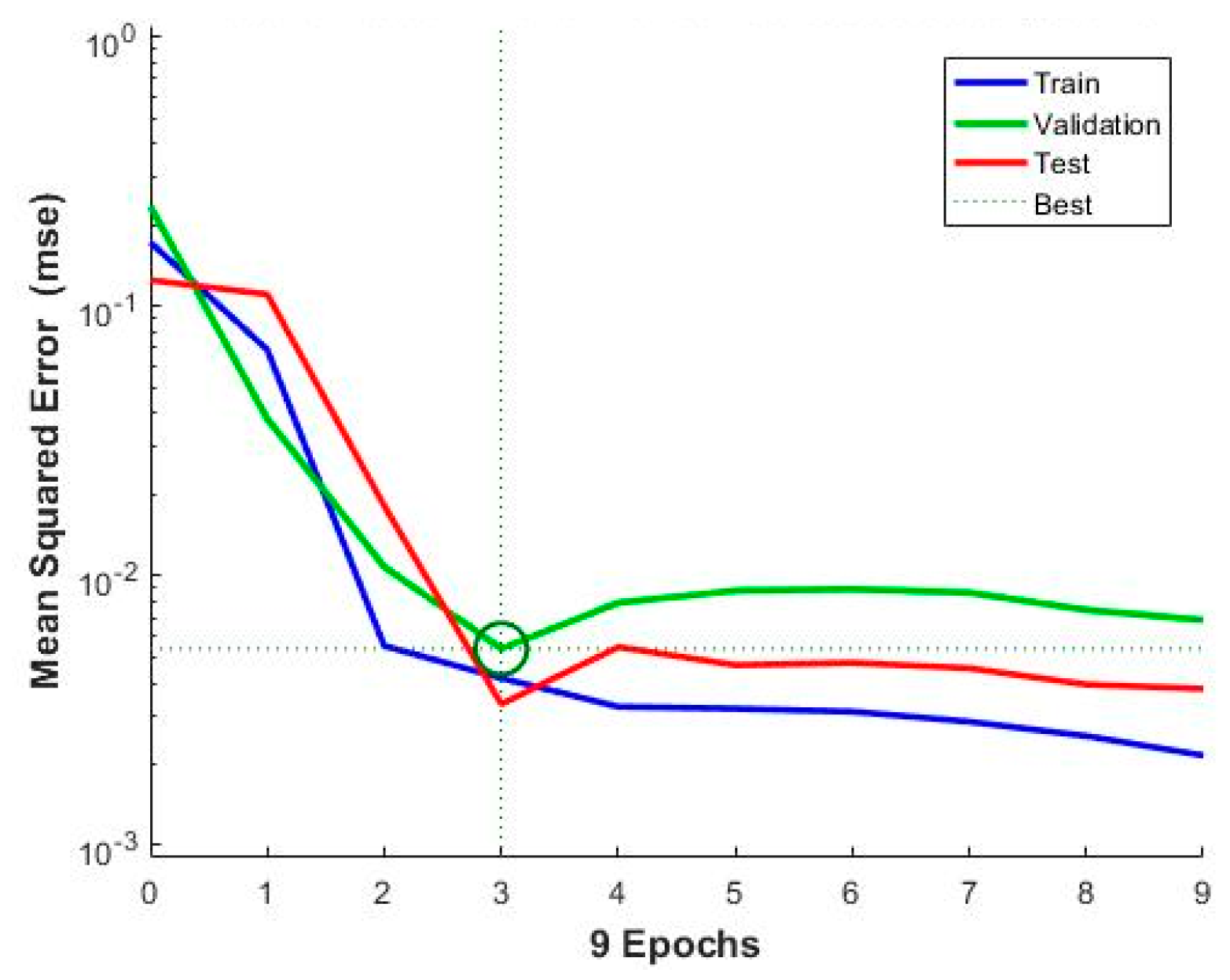
The initiated neural network architecture was then trained using the Levenberg–Marquadt optimization algorithm which employed a backpropagation algorithm. Early stopping was implemented by using 10% to 15% of randomly selected training data as a monitoring set during training. The training stopped after six iterations if no improvement in MSE value was observed for the training dataset compared to the monitoring set to minimize overfitting. The training progression after each iteration is depicted in Figure 3 from the training calibration model for CO2 loading using three molar total MEA datasets. The MSE values for validation and test datasets was observed to decrease from the start before increasing after the third iteration. The training was stopped based on the trends of MSE values for validation data which do not improve after the third iteration. Network parameters at the third iteration were then used for the resulting model.
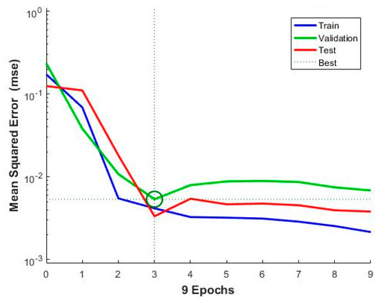
Figure 3.
Plot of mean squared error (MSE) values after each iteration during training.
Ten training runs were conducted per model using randomized initial weights to improve model parameters towards achieving the best possible solution. The trained models were then evaluated based on the calculated MSE values. Adjustments were made on the neural network parameters based on the training results. The model was then retrained with the implemented adjustment and the training process was monitored using validation data. The overall training process for the model concluded once the MSE values stopped improving.
The performance of each developed model was evaluated by assessing the RMSE and coefficient of determination (R2) of the model on the training dataset. R2 value provides an overview of the tightness of the predicted and actual data towards the regression line, while RMSE evaluates the closeness of the predicted value to the actual value. A model with R2 value of above 0.90 indicates excellent correlations between Raman spectrum and species concentration. Also, models with an R2 value of 0.83 to 0.90 are still applicable within a limited scope of use, typically in research work [49].
Selection of the final model parameters was conducted through external validation using the previously split test datasets. Externally validating the model with an independent test dataset allows for unbiased evaluation of the developed calibration model. RMSE for test datasets was compared to the similar RMSE plot for training datasets as observed in the examples in Figure 2 and Figure 3 for PLS and ANN, respectively. The plot shows that the quality of the model does not improve with an additional number of components beyond six, which was consistent with the finding from the scree plot. Further evaluation of R2 was conducted using a test dataset. Additionally, regression plots of the training and test dataset for each calibration model were constructed to analyse the trends in datapoints distribution along the regression line. A total of 21 Raman calibration models were developed using each technique, with seven models each at 3, 4 and 5 molar MEA concentration. The seven models were for protonated MEA, bicarbonate, carbonate, unreacted MEA, carbamate, unreacted CO2, and CO2 loading.
3. Results and Discussion
3.1. Characteristic Bands of Chemical Species in CO2-Loaded Aqueous Monoethanolamine (MEA) System
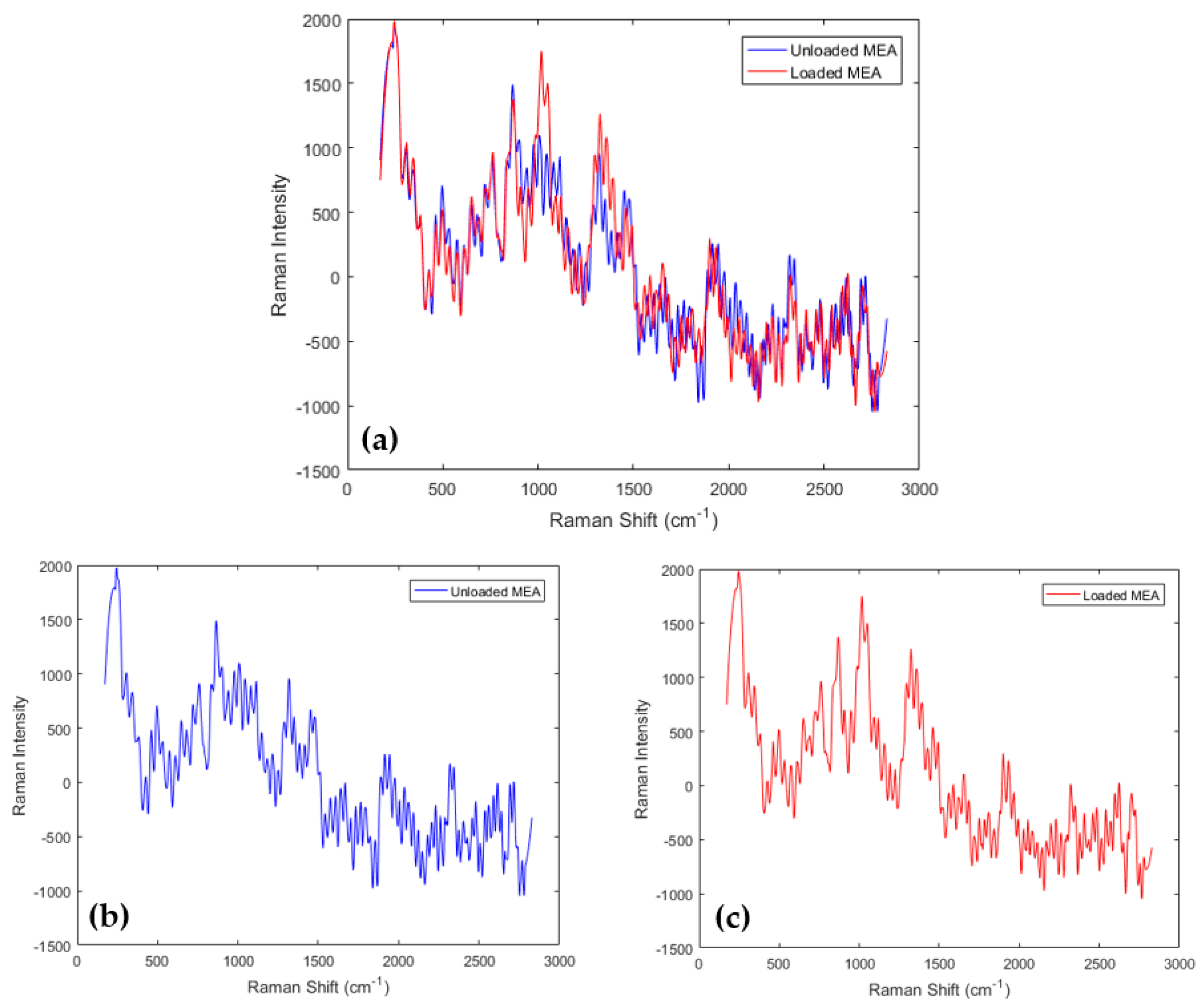
Comparison between the smoothed spectra of the unloaded and the CO2-loaded MEA solution were made as exemplified in Figure 4. Significant peaks were observed at Raman shift range between 800 cm−1 and 1100 cm−1 as well as 1250 cm−1 and 1400 cm−1. The observed peaks were due to changes in species composition caused by CO2 absorption and chemical reactions between species as described in Equations (7)–(11). The ionic species present in the CO2-loaded aqueous MEA solution were protonated MEA, bicarbonate, carbonate, and carbamate while non-ionic species include unreacted MEA and dissolved CO2.
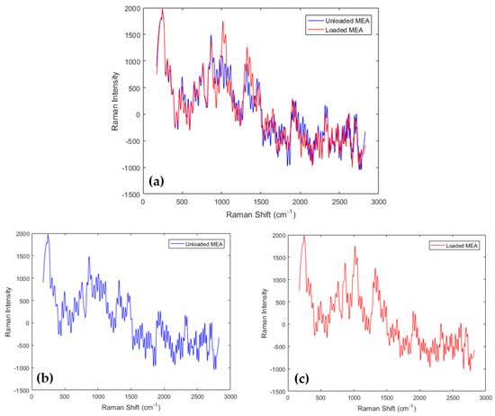
Figure 4.
Plots of Raman spectra captured from unloaded and CO2-loaded aqueous monoethanolamine (MEA) solution. Each are for (a) combined plot, (b) unloaded MEA, and (c) loaded MEA.
For the ionic species, the characteristic band for bicarbonate ion is visible at 1017 cm−1 (C–OH stretching) while the characteristic band for carbonate is located at 1065 cm−1 (C–O bond stretching). The characteristic band for carbamate is observed at 1162 cm−1 (C-N stretching) and for protonated MEA at 1011 cm−1 (CH2 twisting), 1274 cm−1 (C–NH stretch) and 1320 cm−1 (C–C stretch). For non-ionic species, the dissolved CO2 characteristic bands are observed at 1274 cm−1 (CO2 symmetric stretch) and 1383 cm−1 (CO2 bend), while the band for unreacted MEA is observable at 845 cm−1 (CH2 rocking) and 873 cm−1 (CN stretching) [4,6,12,50,51].
It was observed that peak intensity varies at the spectral ranges containing the characteristic bands for the chemical species in the system. In contrast, minimal variations were observed at other spectral ranges. As an example, the Raman spectra in Figure 4 show that spectral intensity at characteristic bands for bicarbonate (1017 cm−1), carbonate (1065 cm−1) and aqueous CO2 (1274 cm−1) increases. The observation agrees with the understanding that ionic species of bicarbonate and carbonate increases in concentration as CO2 loading increases. As the pressure inside the reaction vessel increases, CO2 began to dissolve physically into the solution. The physical dissolution increases aqueous CO2 concentration in the liquid phase. For carbamate, the concentration increases up to a certain point before decreasing as the pressure increases. This follows the theory that carbamate production from the MEA reaction with CO2 limits the capacity for absorption to 0.5 mol of CO2 to mol of amine. As pressure increase, hydrolysis of carbamate forms free amine capable to react with CO2 leading to loading of above 0.5 [23,24].
3.2. Evaluation of the Raman Species Calibration Models
Evaluation on the final Raman calibration models was performed by comparing the coefficient of determination (R2) and RMSE values from the training dataset against the values of the test dataset. The closeness of the R2 and RMSE values between training and test datasets indicate that the model had good generalization towards external data and overfitting is minimal. The overall results for the performance evaluation and validation for PLS and ANN-based calibration models are summarized in Table 3 and Table 4, respectively.

Table 3.
Summary of performance evaluation results for PLS-based Raman species calibration models.

Table 4.
Summary of performance evaluation results for artificial neural network (ANN)-based Raman species calibration models.
It was observed that the R2 values for all calibration models are above 0.90 indicating good fit [49]. For PLS models, the average R2 value is 0.9442 for calibration and 0.9050 for validation while the average RMSE value is 0.1301 for calibration and 0.1583 for validation. As for ANN models, the average R2 value is 0.9505 for calibration and 0.9355 for validation while the average RMSE value is 0.0965 for calibration and 0.1225 for validation. The average value of RMSE for validation (RMSEV) is observed to be higher than RMSE for calibration (RMSEC) while the average value for R2 calibration is higher than R2 validation on both types of model. The observations were due to the use of test data for external validation which carries variance that the model never observed during development. Such an approach was to ensure that the validated model is parsimonious [13,52,53,54]. The differences between the average values were also small, indicating that both PLS and ANN-based calibration models can predict the species concentration in the CO2-MEA-H2O system with good accuracy.
3.3. Comparative Analysis between Partial Least Squares (PLS) and Artificial Neural Network (ANN) Technique for the Development of Raman Calibration Model
Comparisons were made between the final PLS and ANN-based calibration models to determine the technique that produced better performing models. Comparisons were based on the average values of the performance parameters for calibration data. The results are summarized in Table 5.

Table 5.
Comparison between average values of the performance parameters between PLS and ANN models.
Comparing the R2 values, both techniques resulted in comparable calibration models with R2 values above 0.9 indicating a good fit. As for the average RMSE values, ANN-based calibration models have better prediction accuracy compared to PLS-based calibration models. This was indicated by the overall lower average RMSE values observed for all ANN models compared to PLS models. The better performance recorded by ANN is due to the application of the non-linear transfer function that transforms original input into non-linear projection at lower-dimensional subspace. Compared to the linear projection in PLS, the non-linear projection in ANN is more flexible, allowing the ANN model to better fit the datasets. The better fit translates to lower RMSE values for ANN models compared to PLS models [55].
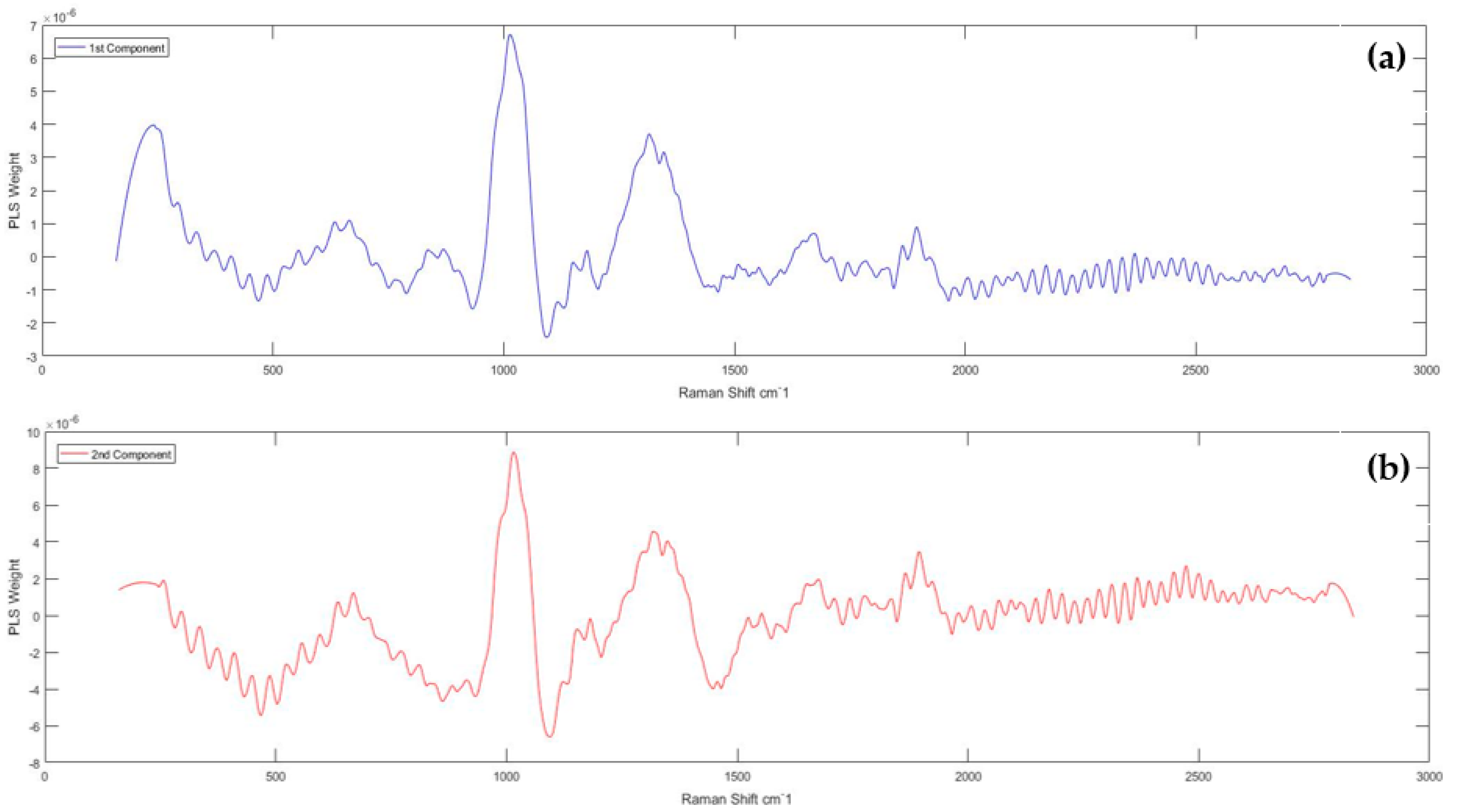
An advantage of applying PLS over ANN is the ability to analyse the model parameters to understand the significance of each Raman variables within the modelled system. It was previously discussed that Raman spectra carry information regarding the chemical species within the monitored system. The information was contained within a specific range of the Raman spectrum called the characteristic band. The characteristic band for a particular chemical species contains spectral variables that are highly correlated with the chemical species. The spectral variables thus contributed highly towards explaining the variance of the species correlated with them in the model. For a PLS calibration model, the contribution was reflected in the PLS weight plot. An example of a weight plot is depicted in Figure 5. The plot was generated from the calibration model of bicarbonate at 4 molar total MEA concentration The plot shows multiple peaks appearing between 500 and 1500 cm−1, indicating that variables within that range are highly correlated to the response variables. The large PLS weight values of the highly correlated variables are evidence that they contribute the most towards the variance explained in the model. The observation is reflective of the literature finding where the characteristic band for bicarbonate is located at 1017 cm−1. Other peaks are from weak intensity signals at 632 cm−1, 1360 cm−1 and 1630 cm−1 due to (OH)CO band, symmetric CO stretching and anti-symmetric CO2 stretch, respectively [56,57].
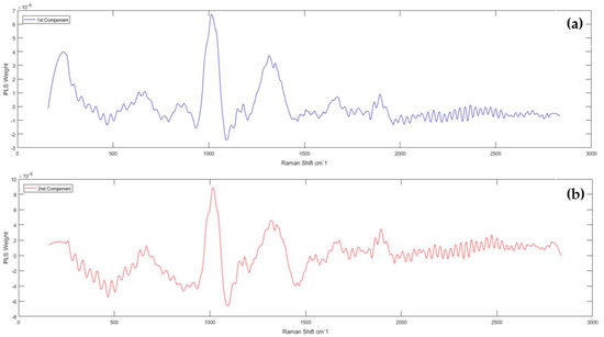
Figure 5.
Weight plots from bicarbonate calibration model (4 molar MEA) for (a) PLS Component 1 and (b) PLS Component 2.
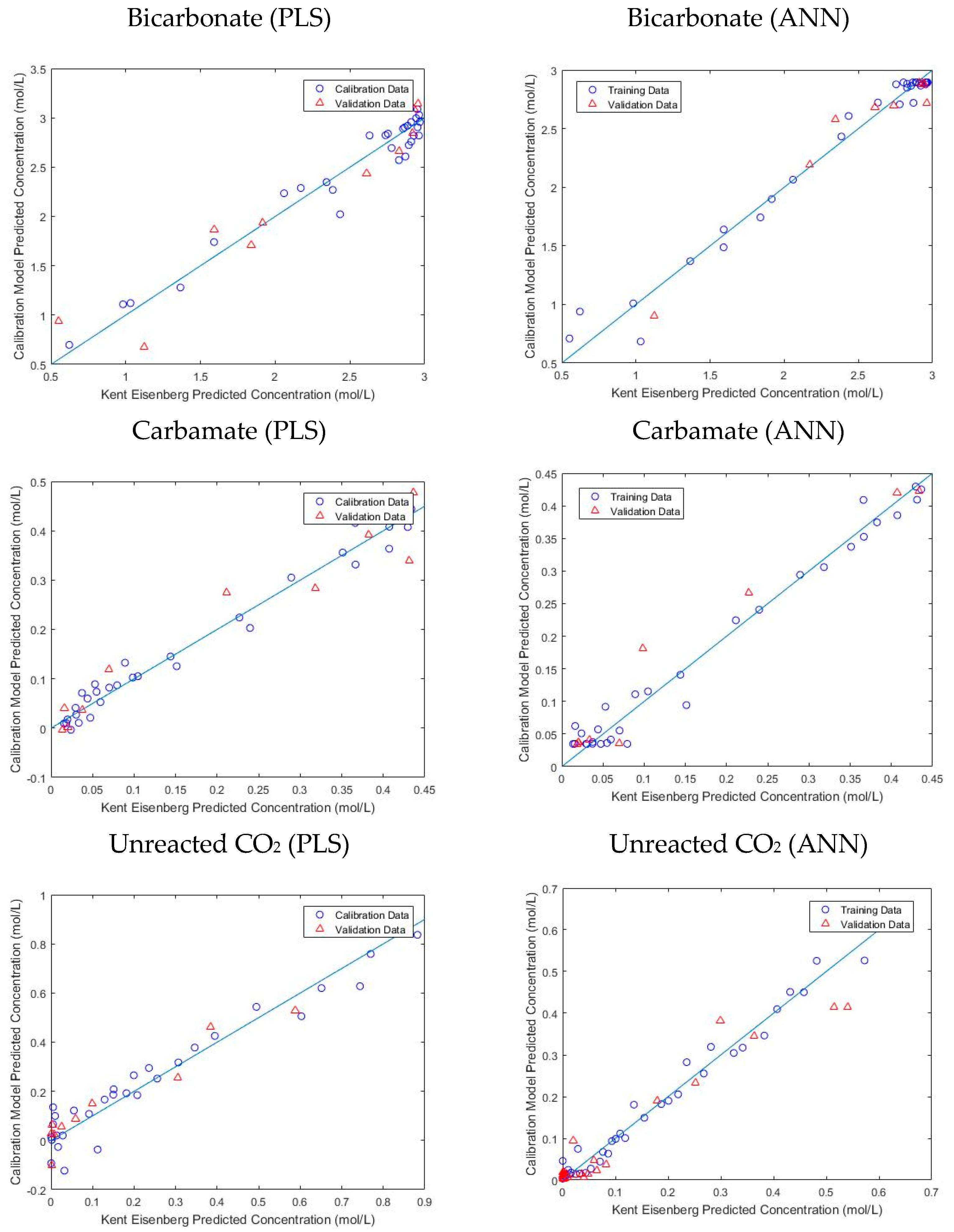
The results from performance evaluation are further supported by observing the regression plots. A good model shall have the datapoints distributed along the regression line. Examples of regression plots are depicted in Figure 6, taken from calibration models for 3 molar MEA concentration. It was observed that the datapoints are well-distributed along the straight line on all models. There was no noticeable trending observed in the distribution of datapoints, indicating that the current model is sufficiently parametrized in explaining the variance in the data. A small deviation was observed between actual and predicted datapoints which was reflected by the resulting RMSEC and RMSEV values.
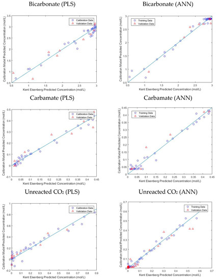
Figure 6.
Regression plots from 3 molar MEA calibration models developed using PLS and ANN techniques.
It was also noted that during the development of the calibration model, the whole spectrum range was utilized. However, the characteristic bands for a chemical species are present only at a specific spectral range within a Raman spectrum based on literature. Other variables outside the spectral range are considered as noises. Developing calibration models by utilizing specific spectral ranges that were correlated with the particular species could reduce noises that interfere during model development thus improving performance [58,59].
4. Conclusions
Development of Raman calibration models utilizing two different multivariate regression techniques, which are partial least squares (PLS) regression and an artificial neural network (ANN), were explored. The Raman spectra and respective species concentration were acquired through the VLE experiment of the CO2-MEA-H2O system at varying total MEA concentration. The VLE data from the experiment were then further used to predict species concentration inside the CO2-MEA-H2O system using the regressed Kent–Eisenberg thermodynamic model. A total of 21 Raman species calibration models were developed using each technique utilizing smoothed Raman spectra and the estimated species concentration. The performance of each model was evaluated using performance parameters of R2 and RMSE. The R2 values from the developed calibration models were above 0.90 while the RMSE values improved throughout model optimization. Comparison of both techniques shows that ANN models were more accurate with lower RMSE values observed compared to the PLS model. However, the small differences between the RMSE values indicate that PLS models were comparatively good in predicting species concentration. Additionally, the PLS model allows studies on the significance of each variable to be conducted through analysing the weight plots, which was not possible in ANN models, this being a black box technique. The regression plots show close data distribution along the regression line with no trending observed from the data distribution for both calibration and test datasets. The result signifies that both techniques are applicable for developing Raman species calibration models to predict species concentration with good accuracy in CO2-loaded aqueous MEA system. Notably, PLS provides added advantages over ANN in terms of analysis on the significance of each spectral variable on the developed models.
Author Contributions
Conceptualization, A.S.H. and A.S.M.; methodology, A.S.H., M.Z.S. and H.S.; validation, A.S.H., A.S.M. and M.Z.S.; formal analysis, A.S.H. and M.Z.S.; investigation, A.S.H.; data curation, A.S.H. and M.Z.S.; writing—original draft preparation, A.S.H.; writing—review and editing, A.S.H., A.S.M., M.Z.S. and H.S.; supervision, A.S.M. and A.B.; funding acquisition, A.S.M. All authors have read and agreed to the published version of the manuscript.
Funding
This research was funded by PETRONAS Research Sdn Bhd, grant number 0153B2-E76. Any opinions and findings as well as conclusions and recommendations made in this material are those of the author(s) and do not necessarily reflect the view of PETRONAS Research Sdn Bhd.
Institutional Review Board Statement
Not applicable.
Informed Consent Statement
Not applicable.
Conflicts of Interest
The authors declare no conflict of interest.
References
- Luis, P. Use of monoethanolamine (MEA) for CO2 capture in a global scenario: Consequences and alternatives. Desalination 2016, 380, 93–99. [Google Scholar] [CrossRef] [Green Version]
- Fan, G.J.; Wee, A.G.H.; Idem, R.; Tontiwachwuthikul, P. NMR studies of amine species in MEA-CO2-H2O system: Modification of the model of vapor-liquid equilibrium (VLE). Ind. Eng. Chem. Res. 2009, 48, 2717–2720. [Google Scholar] [CrossRef]
- Rogelj, J.; Shindell, D.; Jiang, K.; Fifita, S. Mitigation Pathways Compatible with 1.5 °C in the Context of Sustainable Development. In Global Warming of 1.5 °C; An IPCC Special Report; IPCC: Geneva, Switzerland, 2018. [Google Scholar]
- Kachko, A.; van der Ham, L.V.; Bardow, A.; Vlugt, T.J.H.; Goetheer, E.L.V. Comparison of Raman, NIR, and ATR FTIR spectroscopy as analytical tools for in-line monitoring of CO2 concentration in an amine gas treating process. Int. J. Greenh. Gas Control 2016, 47, 17–24. [Google Scholar] [CrossRef]
- Cole, I.S.; Corrigan, P.; Sim, S.; Birbilis, N. Corrosion of pipelines used for CO2 transport in CCS: Is it a real problem? Int. J. Greenh. Gas Control. 2011, 5, 749–756. [Google Scholar] [CrossRef]
- Wong, M.K.; Bustam, M.A.; Shariff, A.M. Chemical speciation of CO2 absorption in aqueous monoethanolamine investigated by in situ Raman spectroscopy. Int. J. Greenh. Gas Control 2015, 39, 139–147. [Google Scholar] [CrossRef]
- Rochelle, G.T. Amine Scrubbing for CO2 Capture. Science 2009, 325, 1652–1654. [Google Scholar] [CrossRef] [PubMed]
- Puxty, G.; Maeder, M. The fundamentals of post-combustion capture. In Absorption-Based Post-Combustion Capture of Carbon Dioxide; Woodhead Publishing: Sawston, UK, 2016; pp. 13–33. ISBN 9780081005156. [Google Scholar]
- Böttinger, W.; Maiwald, M.; Hasse, H. Online NMR spectroscopic study of species distribution in MEA-H2O-CO2 and DEA-H2O-CO2. Fluid Phase Equilib. 2008, 263, 131–143. [Google Scholar] [CrossRef]
- Kontogeorgis, G.M.; Folas, G.K. Thermodynamic Models for Industrial Applications: From Classical and Advanced Mixing Rules to Association Theories; John Wiley & Sons: Hoboken, NJ, USA, 2009; ISBN 9780470747537. [Google Scholar]
- Rinker, E.B.; Ashour, S.S.; Sandall, O.C. Kinetics and Modeling of Carbon Dioxide Absorption into Aqueous Solutions of Diethanolamine. Ind. Eng. Chem. Res. 1996, 35, 1107–1114. [Google Scholar] [CrossRef]
- Souchon, V.; Aleixo, M.D.O.; Delpoux, O.; Sagnard, C.; Mougin, P.; Wender, A.; Raynal, L. In situ determination of species distribution in alkanolamine-H2O-CO2 systems by Raman spectroscopy. Energy Procedia 2011, 4, 554–561. [Google Scholar] [CrossRef] [Green Version]
- Beumers, P.; Brands, T.; Koss, H.J.; Bardow, A. Model-free calibration of Raman measurements of reactive systems: Application to monoethanolamine/water/CO2. Fluid Phase Equilib. 2016, 424, 52–57. [Google Scholar] [CrossRef]
- Smith, E.; Dent, G. Modern Raman Spectroscopy—A Practical Approach; John Wiley & Sons: Hoboken, NJ, USA, 2005; ISBN 9780471497943. [Google Scholar]
- Vogt, M.; Pasel, C.; Bathen, D. Characterisation of CO2 absorption in various solvents for PCC applications by Raman spectroscopy. Energy Procedia 2011, 4, 1520–1525. [Google Scholar] [CrossRef] [Green Version]
- Samarakoon, P.A.G.L.; Andersen, N.H.; Perinu, C.; Jens, K.J. Equilibria of MEA, DEA and AMP with bicarbonate and carbamate: A Raman study. Energy Procedia 2013, 37, 2002–2010. [Google Scholar] [CrossRef] [Green Version]
- Swinehart, D.F. The Beer-Lambert Law. J. Chem. Educ. 1962, 39, 333. [Google Scholar] [CrossRef]
- Matin, N.S.; Remias, J.E.; Neathery, J.K.; Liu, K. Facile method for determination of amine speciation in CO2 capture solutions. Ind. Eng. Chem. Res. 2012, 51, 6613–6618. [Google Scholar] [CrossRef]
- Kent, R.L.; Elsenberg, B. Better Data for Amine Treating. Hydrocarb. Process. 1976, 55, 87–90. [Google Scholar]
- Haji-Sulaiman, M.Z.; Aroua, M.K.; Benamor, A. Analysis of equilibrium data of CO2 in aqueous solutions of DEA, MDEA and their mixtures using the modified Kent Eisenberg Model. Trans. Chem. E 1998, 76, 1–8. [Google Scholar] [CrossRef]
- Suleman, H.; Maulud, A.S.; Man, Z. Carbon Dioxide Solubility in Aqueous Potassium Lysinate Solutions: High Pressure Data and Thermodynamic Modeling. Procedia Eng. 2016, 148, 1303–1311. [Google Scholar] [CrossRef] [Green Version]
- Suleman, H.; Maulud, A.S.; Man, Z. Review and selection criteria of classical thermodynamic models for acid gas absorption in aqueous alkanolamines. Rev. Chem. Eng. 2015, 31, 599–639. [Google Scholar] [CrossRef]
- Sartori, G.; Savage, D.W. Sterically hindered amines for carbon dioxide removal from gases. Ind. Eng. Chem. Fundam. 1983, 22, 239–249. [Google Scholar] [CrossRef]
- Haji-Sulaiman, M.Z.; Aroua, M.K.; Pervez, M.I. Equilibrium concentration profiles of species in CO2—alkanolamine—water systems. Gas Sep. Purif. 1996, 10, 13–18. [Google Scholar] [CrossRef]
- Van Der Maaten, L.; Postma, E.; Van den Herik, J. Dimensionality Reduction: A Comparative Review. J. Mach. Learn. Res. 2009, 10, 66–71. [Google Scholar]
- Hotelling, H. Analysis of a complex of statistical variables into principal components. J. Educ. Psychol. 1933. [Google Scholar] [CrossRef]
- Varmuza, K.; Filzmoser, P. Introduction to Multivariate Statistical Analysis in Chemometrics; CRC Press: Boca Raton, FL, USA, 2009; ISBN 9781420059472. [Google Scholar]
- Wold, S.; Sjöström, M.; Eriksson, L. PLS-regression: A basic tool of chemometrics. Chemom. Intell. Lab. Syst. 2001, 58, 109–130. [Google Scholar] [CrossRef]
- Marini, F.; Bucci, R.; Magri, A.L.; Magri, A.D. Artificial Neural Networks in Chemometrics: History, Examples and Perspectives. Microchem. J. 2008, 88, 178–185. [Google Scholar] [CrossRef]
- Mouazen, A.M.; Kuang, B.; De Baerdemaeker, J.; Ramon, H. Comparison among principal component, partial least squares and back propagation neural network analyses for accuracy of measurement of selected soil properties with visible and near infrared spectroscopy. Geoderma 2010, 158, 23–31. [Google Scholar] [CrossRef]
- Kuang, B.; Tekin, Y.; Mouazen, A.M. Comparison between artificial neural network and partial least squares for on-line visible and near infrared spectroscopy measurement of soil organic carbon, pH and clay content. Soil Tillage Res. 2015, 146, 243–252. [Google Scholar] [CrossRef]
- Ramadan, Z.; Hopke, P.K.; Johnson, M.J.; Scow, K.M. Application of PLS and Back-Propagation Neural Networks for the estimation of soil properties. Chemom. Intell. Lab. Syst. 2005, 75, 23–30. [Google Scholar] [CrossRef]
- Jinadasa, M.H.W.N.; Chandra, K.A.; Halstensen, M. System Development for On-line Monitoring using Raman Spectroscopy for CO2 Absorption by MEA. In Proceedings of the 59th Conference on Simulation and Modelling (SIMS 59), 26–28 September 2018; Oslo Metropolitan University: Oslo, Norway, 2018. [Google Scholar]
- Jinadasa, M.H.W.N.; Jens, K.; Øi, L.E.; Halstensen, M. Raman Spectroscopy as an Online Monitoring Tool for CO2 Capture Process: Demonstration Using a Laboratory Rig. Energy Procedia 2017, 114, 1179–1194. [Google Scholar] [CrossRef]
- Shahid, M.Z.; Maulud, A.S.; Bustam, M.A. Non-invasive monitoring of CO2concentration in aqueous diethanolamine (DEA), methyldiethanolamine (MDEA) and their blends in high CO2loading region using Raman spectroscopy and partial least square regression (PLSR). Int. J. Greenh. Gas Control 2018, 68, 42–48. [Google Scholar] [CrossRef]
- Shahid, M.Z.; Suleman, H.; Maulud, A.S.; Khalil, M.A.B.; Man, Z. Monitoring of Chemical Speciation of DEA-CO2-Water System by Raman Spectroscopy. Adv. Mater. Res. 2015, 1113, 358–363. [Google Scholar] [CrossRef]
- Edwards, T.J.; Maurer, G.; Newman, J.; Prausnitz, J.M. Vapor-liquid equilibria in multicomponent aqueous solutions of volatile weak electrolytes. AIChE J. 1978, 24, 966–976. [Google Scholar] [CrossRef]
- Aroua, M.K.; Salleh, R.M. Solubility of CO2 in aqueous piperazine and its modeling using the Kent-Eisenberg approach. Chem. Eng. Technol. 2004, 27, 65–70. [Google Scholar] [CrossRef]
- Vasques, G.M.; Grunwald, S.; Sickman, J.O. Comparison of multivariate methods for inferential modeling of soil carbon using visible/near-infrared spectra. Geoderma 2008, 146, 14–25. [Google Scholar] [CrossRef]
- Silva, M.A.M.; Ferreira, M.H.; Braga, J.W.B.; Sena, M.M. Development and analytical validation of a multivariate calibration method for determination of amoxicillin in suspension formulations by near infrared spectroscopy. Talanta 2012, 89, 342–351. [Google Scholar] [CrossRef] [PubMed]
- Uysal, R.S.; Boyaci, I.H.; Genis, H.E.; Tamer, U. Determination of butter adulteration with margarine using Raman spectroscopy. Food Chem. 2013, 141, 4397–4403. [Google Scholar] [CrossRef] [PubMed]
- de Jong, S. SIMPLS: An alternative approach to partial least squares regression. Chemom. Intell. Lab. Syst. 1993, 18, 251–263. [Google Scholar] [CrossRef]
- Smits, J.R.M.; Melssen, W.J.; Buydens, L.M.C.; Kateman, G. Using artificial neural networks for solving chemical problems. Part I. Multi-layer feed-forward networks. Chemom. Intell. Lab. Syst. 1994, 22, 165–189. [Google Scholar] [CrossRef] [Green Version]
- Hornik, K.; Stinchcombe, M.; White, H. Multilayer feedforward networks are universal approximators. Neural Netw. 1989, 2, 359–366. [Google Scholar] [CrossRef]
- Svozil, D.; Kvasnička, V.; Pospíchal, J. Introduction to multi-layer feed-forward neural networks. Chemom. Intell. Lab. Syst. 1997, 39, 43–62. [Google Scholar] [CrossRef]
- Pearson, K. LIII. On lines and planes of closest fit to systems of points in space. Lond. Edinb. Dublin Philos. Mag. J. Sci. 1901, 2, 559–572. [Google Scholar] [CrossRef] [Green Version]
- Janik, L.J.; Cozzolino, D.; Dambergs, R.; Cynkar, W.; Gishen, M. The prediction of total anthocyanin concentration in red-grape homogenates using visible-near-infrared spectroscopy and artificial neural networks. Anal. Chim. Acta 2007, 594, 107–118. [Google Scholar] [CrossRef] [PubMed]
- Despagne, F.; Massart, D.L. Neural networks in multivariate calibration. Analyst 1998, 123, 157R–178R. [Google Scholar] [CrossRef] [PubMed]
- Williams, K. Near-infrared technology in the agricultural and food industries. In Near-Infrared Technology in the Agricultural and Food Industries; American Association of Cereal Chemists, Inc.: Saint Paul, MI, USA, 2001; ISBN 1-891127-24-1. [Google Scholar]
- Batista de Carvalho, L.A.E. Raman spectra, conformational stability and normal coordinate analysis of ethylmethylamine. J. Raman Spectrosc. 1995, 26, 653–661. [Google Scholar] [CrossRef]
- Larkin, P. IR and Raman Spectra-Structure Correlations. In Infrared and Raman Spectroscopy; Elsevier: Amsterdam, The Netherlands, 2011; ISBN 9780128041628. [Google Scholar]
- Salciccioli, J.D.; Crutain, Y.; Komorowski, M.; Marshall, D.C. Sensitivity analysis and model validation. In Secondary Analysis of Electronic Health Records; Spring: Berlin/Heidelberg, Germany, 2016; ISBN 9783319437422. [Google Scholar]
- Alpaydin, E. Introduction to Machine Learning; MIT Press: Cambridge, MA, USA, 2014; ISBN 0262325748. [Google Scholar]
- Posada, D.; Buckley, T.R. Model selection and model averaging in phylogenetics: Advantages of akaike information criterion and bayesian approaches over likelihood ratio tests. Syst. Biol. 2004, 53, 793–808. [Google Scholar] [CrossRef]
- Bakeev, K.A. Process Analytical Technology: Spectroscopic Tools and Implementation Strategies for the Chemical and Pharmaceutical Industries: Second Edition; John Wiley & Sons: Hoboken, NJ, USA, 2010; ISBN 9780470722077. [Google Scholar]
- Davis, A.R.; Oliver, B.G. A vibrational-spectroscopic study of the species present in the CO2-H2O system. J. Solut. Chem. 1972, 1, 329–339. [Google Scholar] [CrossRef]
- Wen, N.; Brooker, M.H. Ammonium carbonate, ammonium bicarbonate, and ammonium carbamate equilibria: A raman study. J. Phys. Chem. 1995, 99, 359–368. [Google Scholar] [CrossRef]
- Axrup, L.; Markides, K.; Nilsson, T. Using miniature diode array NIR spectrometers for analysing wood chips and bark samples in motion. J. Chemom. 2000, 14, 561–572. [Google Scholar] [CrossRef]
- Xu, F.; Wang, D. Rapid determination of sugar content in corn stover hydrolysates using near infrared spectroscopy. Bioresour. Technol. 2013, 147, 293–298. [Google Scholar] [CrossRef]
Publisher’s Note: MDPI stays neutral with regard to jurisdictional claims in published maps and institutional affiliations. |
© 2021 by the authors. Licensee MDPI, Basel, Switzerland. This article is an open access article distributed under the terms and conditions of the Creative Commons Attribution (CC BY) license (https://creativecommons.org/licenses/by/4.0/).

