Dynamically Operated Fischer-Tropsch Synthesis in PtL-Part 1: System Response on Intermittent Feed

Abstract

Society is facing serious challenges to reduce CO₂ emissions. Effective change requires the use of advanced chemical catalyst and reactor systems to utilize renewable feedstocks. One pathway to long-term energy storage is its transformation into high quality, low-emission and CO₂-neutral fuels. Performance of technologies such as the Fischer-Tropsch reaction can be maximized using the inherent advantages of microstructured packed bed reactors. Advantages arise not only from high conversion and productivity, but from its capability to resolve the natural fluctuation of renewable sources. This work highlights and evaluates a system for dynamic feed gas and temperature changes in a pilot scale Fischer-Tropsch synthesis unit for up to 7 L of product per day. Dead times were determined for non-reactive and reactive mode at individual positions in the setup. Oscillating conditions were applied to investigate responses with regard to gaseous and liquid products. The system was stable at short cycle times of 8 min. Neither of the periodic changes showed negative effects on the process performance. Findings even suggest this technology’s capability for effective, small-to-medium-scale applications with periodically changing process parameters. The second part of this work focuses on the application of a real-time photovoltaics profile to the given system.

1. Introduction

The Fischer-Tropsch synthesis (FTS) is a polymerization type reaction, which converts synthesis gas (hydrogen and carbon monoxide) into many different hydrocarbons; ranging from methane to carbon chains with over 100 carbon atoms. Those products can be distinguished as gases, liquids or solids under ambient conditions. Water is produced as a byproduct of the reaction. Synthesis products can be applied for many different applications in the energy, chemical and material industry. Middle distillate type hydrocarbons can be utilized as synthetic fuels for a multitude of vehicles and vessels that are designed for operation with fossil fuels. Specific metal surfaces are necessary to boost the reaction rate and to optimize the chain distribution, which makes the FTS a prominent example for heterogeneous catalysis. The reaction equation, based on synthesis gas to produce linear alkanes, is shown in Equation (1) [1,2,3]:

(2n + 1)H₂ + nCO → C_nH_2n+2 + nH₂O.

(1)

This synthesis is influenced by a myriad of different process parameters such as the catalyst and support system, temperature, partial pressures, residence time and overall feed gas composition and dilution, as well as conversion levels [4,5,6,7]. All of those characteristics have been intensively investigated in the history of the FTS [2,6,8,9]. Investigations regarding process properties for the cobalt-based catalyst used in this work have been executed before [10,11,12,13,14,15]. Figure 1 shows a typical carbon chain length distribution of the FTS products. They mainly consist of linear alkanes, alkenes and iso-alkanes, as well as alcohols [2,16,17,18,19].

1.1. Energy Transition and Technologies that May Be Required

In the context of energy transition, humanity aims to mitigate climate change, which is strongly influenced by the amount of anthropogenic CO₂ emissions [20]. In terms of efficiency, technological advances must help to achieve a reduction of energy demand per capita and overall consumption of goods [21,22,23,24]. While the world’s CO₂ emission from crude oil utilization is almost constant over the past two decades, the transport sector has significantly increased its share from 22% in 1990 to 28% in 2016 [25]. Finding and applying sustainable alternatives is thus necessary.

Many different pathways to substitute fossil fuel with CO₂-neutral sources have opened up in recent years. Most of them rely on renewable electrical energy from wind, solar and hydropower. Whenever possible, the generated electricity should be directly used or can be converted into heat. It can also be used for transportation and manufacturing of materials, with given conversion losses [26,27]. Those technological pathways can be summarized as power-to-X (PtX) or, more specifically, power-to-liquid (PtL) and power-to-gas (PtG) processes. Generally, there will be a need for different energy storage technologies in a highly volatile and fluctuating renewable energy system [26,28,29,30,31]. A good share of the renewable energy will be exploitable under certain conditions. Energy from the sun can only be harvested at daytime and is best with good weather. Wind energy delivers more power when strong winds are present. Even hydropower from sea streams and rivers shows different performance profiles based on seasonal influences and water levels. In the end, with increasing use of renewable electricity, the overall fluctuation generates grid instabilities and the energy demand cannot be fulfilled at all times [32,33].

Thus, the two biggest challenges for the future energy grid are the storage of surplus energy and filling up the gaps in times of an undersupply. This is known as the intermittency problem [27,33,34,35,36,37,38,39]. The consequence is the need for storages that deplete in times of undersupply and can be filled in times of overproduction. Those storages need to work as a buffer system between the producer and the consumer. Storages come at a certain price [37,38,40,41].

In terms of batteries, the volumetric energy density is problematic on long distances and with heavier masses to be transported. They are thus less suitable for heavy duty or air transport [6,42,43]. The high demand for lithium and cobalt for a global supply and the limited capacity of batteries are further reasons not to completely rely on electric mobility as the predominant form of transportation [6].

Gaseous products offer a higher level of chemical availability from the respective molecule’s inherent energy, but storage and product handling are quite difficult in terms of safety, cost and storage size [44,45,46]. Transportable gases need to be either condensed at low temperature or compressed, which adds cost to the overall process. Hydrogen is the most expensive to store due to its low density and condensation temperature. Still, it is necessary in most synthesis routes [45,46].

Liquid chemicals are a good energy storage due to their high volumetric energy density. This enables good transportability with low tank weight.

In order to cover the need for energy and materials, a full range of applicable technologies needs to be mixed and organized in an intelligent way. As one of many demonstration platforms in that regard, the “Energy Lab 2.0” was erected in the Helmholtz Association with funding of BMWi, BMBF and the State of Baden-Württemberg in Germany. This infrastructure looks into the real-time behavior of energy producers, converters and consumers [47]. The aim is to manage energy and to distribute it over many different pathways, such as power-to-heat (PtH), PtL and PtG. A number of different PtL projects use this platform to investigate sector coupling. Figure 2 is an example of a PtL-approach as a framework of the studies done in this work.

The Fischer-Tropsch reaction in the PtL pathway shows high potential to produce synthetic substitutes for fossil fuels in already existing, efficient engine systems [48,49]. Distribution would be possible without new infrastructure, since refineries and fueling stations could be used without much additional cost [3]. The liquid fuel shows better combustion properties in terms of soot and NO_x emissions and does not contain poisons, contaminants or aromatics, unlike fossil fuels [48,49,50].

Still, there are a number of reasons why this pathway has not been exploited yet. The most important one is the economic comparison between the costs of synthetic and fossil fuels. The synthetic pathway has always been considerably more expensive [51]. In times of ecological awareness and a changing energy system, this might easily change if CO₂ emission cost increase and synthetic fuels become recognized as carbon-neutral fuels [43,52,53].

The second main reason is technological limitation. The few technical plants installed worldwide operate with restricted reaction performance. Avoiding hot spots in the catalyst due to limited heat management or mass transfer limitation between reactants and catalysts are the main reasons [54]. Those compromises are evened out by economy of scale, for which a huge continuous feed is needed. This favors large installations as well as a large, centralized infrastructure [3,6]. Also, state-of-the-art technology would rely on large storage and buffer systems [46,55]. With advanced reactor systems, a broader application of this technology in smaller scale seems viable nowadays [54,56,57].

One idea to tackle the issues of buffer costs is to reduce their size by operating a dynamic synthesis with a flexible energy input. This may only be realized by advanced process control and modular approaches.

1.2. Microstructured Reactor Technology

In the last decade, the development of microstructured (packed bed) reactors enabled intensification of processes due to increased heat and mass transfer [10,11]. In regard to FTS, microstructured packed bed reactors constitute the most developed available technology to maximize the reaction output by overcoming state-of-the-art limitations and concerns [11,56,58,59,60,61,62]. Small interior dimensions drastically increase the surface area and local heat transfer. Higher conversion levels can be applied in the process without harming the catalyst. Furthermore, concentration and temperature changes may be quickly applied because of short overall distances and advanced tools like evaporation cooling [61,63,64,65]. This allows high-pressure steam production from the FTS reaction in order to enhance the thermal efficiency of a process network while enabling the control over the FTS reactor at the same time.

Additionally, the small interior dimensions of microstructured devices enable a broad scalability of the overall process that is not accessible with conventional solutions—decentralized small-scale applications become cost-competitive due to reduced transport distances. Advantages also include improved reaction safety through small reaction inventory [6,11,66].

Microstructured reactors have already been successfully implemented into the market for small--to-medium-scale applications [54,67,68]. They could also be used in additional processes (e.g., island solutions for local energy conversion).

Concluding, FT fuel may be a viable and competitive high-performance fuel besides obvious conversion losses that every multi-step synthesis must face. Microstructured packed bed reactors are advantageous for FT synthesis and may open up the possibility to operate the synthesis according to the fluctuating nature of renewable sources.

Nevertheless, unresolved technical questions need to be answered at this point. Those are:

• What knowledge is needed for controlling a dynamic process in small-to-medium-size businesses?
• Can all different process steps be aligned in dynamic operation? What are their general limitations?
• What is the potential to reduce storages through dynamic synthesis?
• What are considerable “dynamic time periods” and ramping scenarios that plants need to tolerate?
• Can the prerequisites from “dynamic time periods” be met by reactors and/or plants?
• How is overall higher efficiency correlated to values of buffer reduction?

In the scope of this manuscript and the following part two, most of the above questions will be addressed from the point of view of a microstructured FT reactor. However, to fully answer these questions, information from other steps, i.e., from hydrogen generation to syngas production, need to be included.

2. Materials and Methods

2.1. Analysis in Transient and Steady-State Operation

The steady-state analysis of the product phases, applied also in this study, is based on gas chromatography (GC) of the individual phases and the gravimetric measurement of liquid and solid phases. Details are explained in previous publications from our group [10,11,12,13,14]. Calculation of weight hourly space velocity (WHSV), the chain growth probability (α), conversion levels, selectivity, and productivity are described in detail there as well; those calculations do not differ from methods widely used in literature.

However, since regular GC analysis is too slow for analyzing transient experiments, a mass spectrometer (MS) was additionally used to measure gaseous products in intervals of several seconds, which is a justified time period for process changes below the minute-scale. The used device (V&F, Germany) applies standard electron impact ionization for hydrogen and chemical ionization to avoid fragmenting of larger molecules. It consists of three main parts:

• A Diluter 004 that dilutes the sample with Ar to avoid detector overloading (below 500,000 counts s⁻¹). Measurements were performed at 1:20 up to 1:30 dilution. Pressure fluctuation from 0.02–0.5 MPa can be compensated.
• An Airsense 2000 unit that can apply three different gases (or mixtures thereof) with different ionization energies: Hg (10 eV), Xe (12 eV) and Kr (14 eV); these gases can be switched within several milliseconds. Electron impact ionization is used to generate primary ions; those ions hit sample molecules and transfer their charge. A quadrupole high-frequency mass filter then separates gaseous molecules based on their mass number (0–500 amu) while the sample can be continuously measured with an impact detector using pulse counting electronics. Depending on the switching times of the quadrupole, the ionization gas and the required number of signals, the interval for a new measurement can range between < 1 s and several seconds. For detecting CO, CO₂, CH₄, and C₃H₈, approximately 3 s were needed to apply a mixture of Xe and Kr.
• An H-Sense unit where the sample is ionized via electron impact ionization so the concentration of H₂ can be measured in response times below 300 ms.

2.2. Experimental Test Rig

The pilot scale test rig is detailed elsewhere [15]. In brief, it consists of

(1)

a gas feeding system with mass flow controllers (MFCs; Brooks, NL),

(2)

a microstructured pilot scale reactor with evaporation cooling in patented design (Figure 3) and a reaction volume of approx. 150 cm³ designed to produce around 7 L of liquid product per day, depending on the process conditions; it was filled with 120 g commercial catalyst with 20 wt.% CO on optimized alumina,

(3)

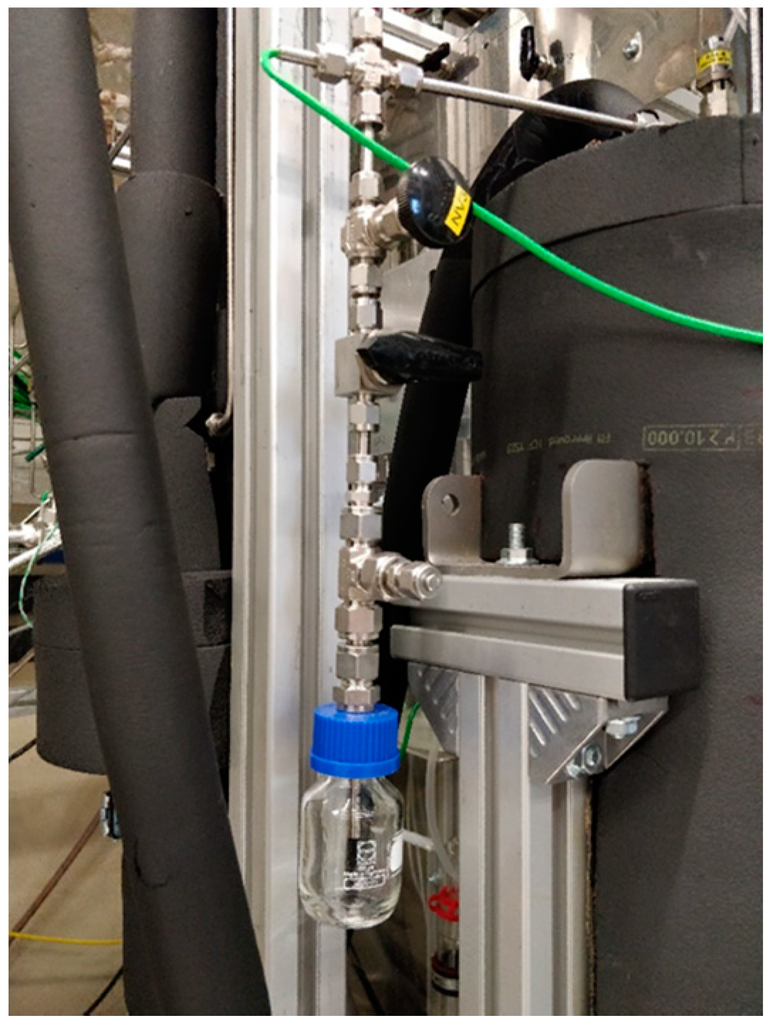
a hot trap (HT) and cold trap (CT) to capture the different product phases; a micro-heat exchanger (µHE) cools down the stream between both traps (Figure 4).

Gaseous products are measured online via GC after a backpressure regulator. The setup is almost identical to previous publications [11,13,15] except for the Quick Sampling (QS) site (see Section 2.4). Setup, reactor and catalyst were operated for approx. 6500 h before the experiments in this work, mostly in standby mode but also several hundred hours of FTS reaction. In standby mode, small amounts of H₂ and N₂ were dosed at 170 °C reactor temperature to preserve the catalyst from oxidation.

2.3. Residence Time Distribution and Dead Time Measurements (Non-Reactive and Reactive Mode)

The determination of the residence time distribution (RTD) is an important criterion for the characterization and description of any chemical plant [69,70,71,72,73]. It indicates the average residence time and potential back-mixing of molecules in the reaction apparatus and system periphery. Knowledge of the RTD is of utmost importance in unsteady-state operation as back-mixing is taking additional influence on time-resolved product composition and on composition of recycle streams.

The RTD is influenced by molecular diffusion, shear forces and forced convection depending on laminar or turbulent conditions and on geometric designs of an apparatus. It is usually determined through tracer experiments. A marker substance is added to the inlet flow, which is then observed at the outlet. Two approaches are usually chosen to introduce a tracer; a pulse or a displacement marking. In this work, the latter strategy was the method of choice, since changes in the feed gas concentration are similar to displacement and can be described accordingly [74].

The sum function F(t) indicates the share of the tracer that has already left the investigated system as a function of time t. It is directly accessible from a displacement marking. The common definition of the first momentum µ₁ is used according to Equation (2) to define the average residence time τ calculated from F(t), [74]

$${\mu }_1=\tau ={{\displaystyle \int }}_0^{1}t dF\left(t\right).$$

(2)

The MS was used to measure the F curve and a dead time without reaction (non-reactive) by adding CO₂, for details see below. The dead time is defined as the time where the signal approaches a constant value i.e., F(t) = 1. It was measured before the reactor and after each major system component, which includes the volume of tubing in between (see Figure 5).

The respective volumes between each location of measurement are listed in

Table 1. List of volumes and applied temperature levels for the main components of the test rig.

System Component	Volume (L)	Temperature (°C)
Reactor	0.15	220–250
HT/µHE CT	4.8 25	170 10

.

Inert tracer experiments [75,76] were conducted with a total flow of 19 L min⁻¹ hydrogen at 3 MPa; total flow and pressure are similar to values in reactive mode (see Table 3). To keep the total flow rate, an additional flow of 1 L min⁻¹ of nitrogen was replaced by CO₂. After detecting 5 vol.% at the outlet, the gases were switched again. Three repetitions were carried out for each location in the test rig.

Table 2. List of parameters for response measurements in non-reactive and reactive mode.

Mode	Setup	Total Gas Flow (L min−1)	H2 Content (vol.%)	N2 Content (vol.%)	CO Content (vol.%)	CO2 Content (vol.%)	Temperature (°C)	Pressure (MPa)	H2/CO (-)
Non-reactive	CO2 on/off	20	95	5/0	0	0/5	225	3	-
Reactive	H2/CO high	17	50	25	25	0	238	3	1.95
Reactive	H2/CO low	17	35	40	25	0	237	3	1.38

gives an overview over the adjusted parameters for RTD and dead time measurements in non-reactive mode. It also shows the threshold values of H₂/CO (“high” and “low” ratio), which were switched back and forth, in reaction experiments (reactive mode) to compare with results from non-reactive measurements (see also Section 2.5).

2.4. Quick Liquid and Gas Sampling (QS)

Since the CT is the largest vessel in the system with a volume of about 25 L, a quick liquid sampling (QS) was a prerequisite to avoid large back-mixing of gas as well as liquid in the vessel and to be able to detect gas phase changes in reaction experiments. Gas sampling before the hot trap would not have been possible due to potential damage of the MS from condensation of wax and liquid components inside the device. In Figure 6, the installation of the QS site is shown. Basically, it represents a glass vessel capable to collect a few milliliters of liquid in a minute-scale sampling time. It could be connected via a needle valve to the effluent of the heat exchanger at a certain point in time. The accompanied gaseous products entering the QS were directed to the MS during the time when the liquid samples were captured. The needle valve was opened into a certain position to avoid pressure loss in the setup.

2.5. Dynamic Profiles by Oscillation of Feed Concentration

For switching the gas composition under the reaction, two different parameter combinations were chosen, see also

Table 3. Average alcohol content in FTS water measured by GC-FID as an average of 18 randomly selected water samples. Residual uncalibrated signal areas are also given.

Species/Property	Concentration
Methanol	14.19 ± 4.14 g L−1
Ethanol	4.64 ± 1.44 g L−1
Propanol	1.21 ± 0.32 g L−1
Butanol	0.79 ± 0.27 g L−1
Pentanol	0.66 ± 0.19 g L−1
Hexanol	0.23 ± 0.06 g L−1
Heptanol	0.07 ± 0.02 g L−1
Total concentration	21.78 ± 6.04 g L−1
Uncalibrated peaks	7.41 ± 2.10 %

. The syngas ratio was significantly changed from 1.95 (“H₂/CO high”) to 1.38 (“H₂/CO low”) in those settings so that a measurable change in the product composition could be expected [6,76]. At this point, the ratio was not lowered further in order not to force deactivation of the catalyst by high hydrogen consumption at increasing CO partial pressure. The length of each oscillation cycle was selected based on the dead time experiments.

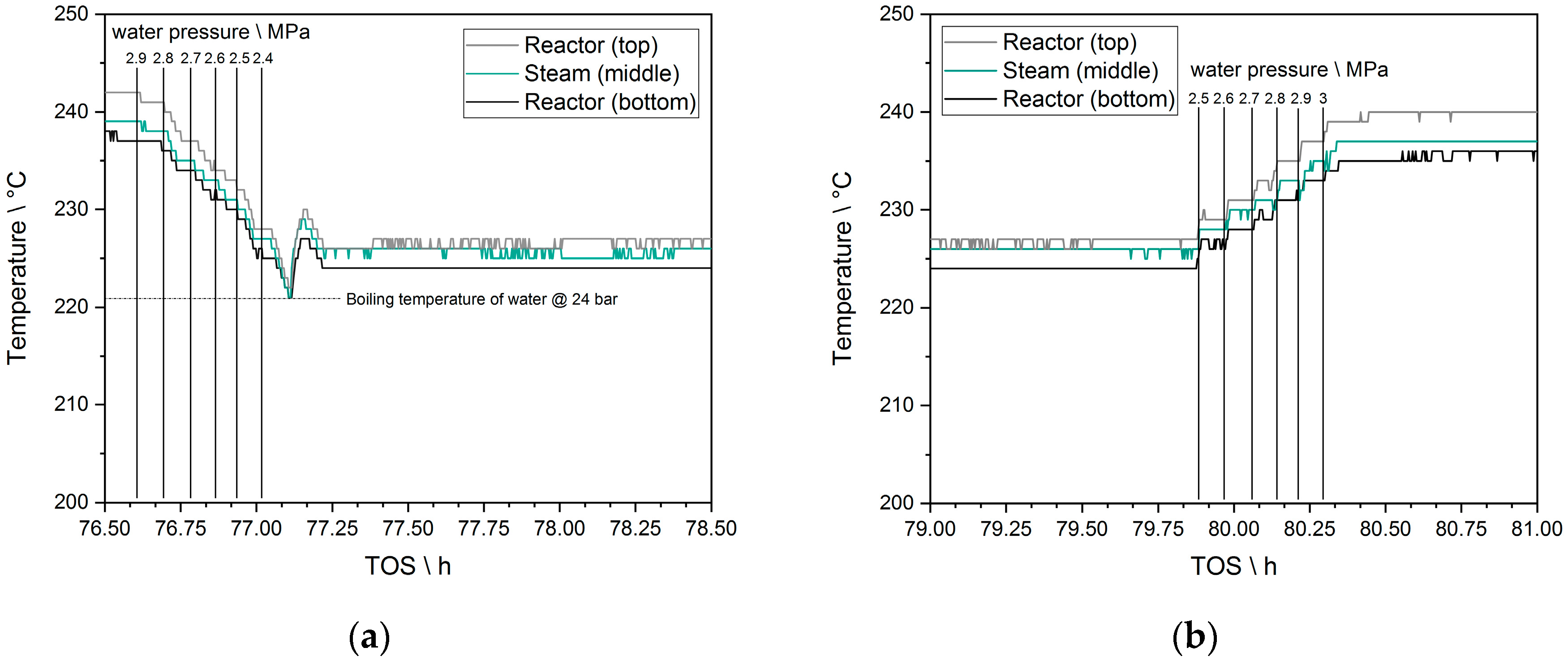
2.6. Evaporation Cooling as a Tool for Influencing the Reactor Temperature

Besides their potential ability to cope with quick changes of feed gas concentration due to a good plug flow type behavior in gaseous fluids, microstructured reactors further possess a high flexibility with regard to temperature changes due to the good heat transfer properties. This might be even more valid when evaporation cooling is applied since the reaction temperature could be manipulated with the evaporation conditions. Absolute pressure determines the boiling temperature in the water-steam system. The temperature is constant as long as both phases exist, thus, water is always fed in excess compared to the evolving reaction heat. Overheating of steam should be avoided due to the small specific heat capacity of steam [15,77]. Equation (3) shows the maximum amount of heat flux ($\Delta {\dot{H}}_{max}$) that liquid water may take up from starting temperature T₀ to boiling temperature T_b, over fully evaporating and overheating to temperature T_end.

$$\Delta {\dot{H}}_{max}={\dot{m}}_{H_{2}O} · c_{p,l} ·\left(T_b-T_0\right)+{\dot{m}}_{H_{2}O} · \Delta h_v+{\dot{m}}_{H_{2}O} · c_{p,g} ·\left(T_{end}-T_b\right)$$

(3)

with ${\dot{m}}_{H_{2}O}$ being the mass flow of water (g s⁻¹), $c_{p,l}$ being the specific heat capacity of liquid water (J g⁻¹ K⁻¹), $\Delta h_v$ being the specific evaporation enthalpy of water (J g⁻¹), and $c_{p,g}$ being the specific heat capacity of steam (J g⁻¹ K⁻¹).

Figure 7 depicts the relationship between the pump’s water mass flow and the resulting enthalpy it could potentially take up. The theoretical vapor fraction is also shown, assuming the total reaction enthalpy is transferred to the water. An average reaction enthalpy from about 30 different experimental conditions is displayed for comparison. The reaction enthalpy ΔH_R (W) was calculated based on Equation (4) from the standard reaction enthalpy ΔH_R⁰ (−158.5 kJ mol⁻¹), CO conversion X_CO (-) and the molar feed flow of CO, ${\dot{n}}_{CO, in}$ (mol s⁻¹).

$$\Delta H_R=\Delta H_R^0·{\dot{n}}_{CO, in}·X_{CO}.$$

(4)

Experiments showing the system’s cooling functionality have been conducted before [15]—a typical water mass flow, which has been set, ranged between three 3 and 4 kg/h.

Excess water, in an average operation case of the pilot scale reactor above a required minimum water mass flow of approximately 1.5 kg h⁻¹, can remove additional heat in a phase of cooling down the reactor. This heat is originating from the total heat capacity of the reactor. A strategy to reduce the reactor temperature could thus be to lower the pressure. Experiments to determine the reactor temperature response by changing water pressure have been carried out in this work. The water pressure was adjusted from 3 MPa to 2.4 MPa and back to 3 MPa by changing 0.1 MPa of pressure every 5 minutes while observing changes in the measured temperatures.

3. Results and Discussion

3.1. General Product Composition and Comparison to Quick Sampling

Product water is collected in the cold trap and is separated manually from the liquid FTS product (oil phase). There were several hydrocarbon species identified in this water. The average concentration of alcohols that could be analyzed from methanol to heptanol accounted for 21.78 g L⁻¹ (±6.04 g L⁻¹) representing 18 randomly selected water samples. Table 3 gives an overview of the alcohol concentrations for calibrated species measured by GC applying the flame ionization detector (FID) signal. Residual 7.41% of the total signal area corresponds to uncalibrated peaks. Alcohol formation is strongly dependent on the process parameters, thus the large given average deviation.

Average product properties of 51 FT oil samples collected in the cold trap and the average chain growth probability, are listed in

Table 4. Average sample composition and chain growth probability α of FT oils determined from 51 samples collected in the CT.

Property	Content/Value
Av. alkane content (oil)	78.18 ± 3.21 wt.%
Av. alkene content (oil)	14.14 ± 4.03 wt.%
Av. iso-alkane and alcohol content (oil)	7.69 ± 1.78 wt.%
Av. carbon chain length (oil)	10.71 ± 0.79 atoms
Av. probability of chain growth (α)	88.44 ± 1.53%

. Alcohols and iso-alkanes in the oil fraction could not be separated in the applied GC method. For that reason, those values are provided as sum.

The detected alcohols are valuable products as they possess a high octane number, which is applicable for gasoline substitution [49]. It must be decided economically if the upgrading and separation process is viable at this point. Iso-alkenes are favorable for cold-flow properties of diesel and kerosene substitution; alkenes generally need to be converted by hydrogenation to reduce degradation effects in liquid storage or during distillation. N-alkanes and iso-alkanes possess good combustion properties with regard to low soot formation.

Previous to the cycling experiments it was checked in stationary reaction conditions whether the QS samples differ or not from the CT sample as a function of the QS sampling time. A certain discrepancy between the samples’ characteristics could be observed (

Table 5. Illustrative sample composition of FT oil from 5 min sampling at QS site and a sample taken at the CT. Stationary reaction conditions 245 °C, 3 MPa total pressure, a H₂/CO ratio of 1.96, and a WHSV of 4.37 h⁻¹.

Property	QS	CT
Alkane content (oil)	80.22 wt.%	75.77 wt.%
Alkene content (oil)	9.50 wt.%	17.70 wt.%
Iso-alkane and alcohol content (oil)	10.28 wt.%	6.53 wt.%
Carbon chain length (oil)	11.47 atoms	9.56 atoms

).

Around 5 min of sampling time at the QS site was required to obtain enough liquid sample for analysis. A longer sampling of e.g., 8 min showed no difference to 5 min samples, but pressure loss in the reaction setup occurred, which is not tolerable for the experiments. Thus, 5 min of sampling time was chosen for all experiments.

Additionally, cooling of the QS site was performed similar to the conditions at the CT (10 °C) to see if there is an effect of flashing temperature. However, the cooling had no effect on the composition of the sample. Thus the flashing pressure is most likely the reason for a shorter average chain length in the CT samples. While reducing the pressure in the QS site to around 0.1 MPa, the CT operates at 30 MPa in which the equilibrium conditions of the gas-liquid system are different. At lower total pressure, the partial pressure of all species is reduced; this lowers not only the overall liquid amount but also shifts the composition towards smaller molecules in the gas phase and consequently leads to a larger average chain length in the QS sample. Solubility effects may also play a role influenced by the equilibration time, which could explain the different alkene and isomer content. In the CT, the time for equilibration is much longer.

As mentioned in Section 2.1, online GC analysis of the product gas takes too long for a proper resolution in dynamic operation. Although resolution is enhanced by MS, the combination of species in the effluent gas and the typical drift of the MS system led us to the conclusion that a calibration of the individual signals is not straightforward. Instead, an analysis of the changes by MS during the change of reaction conditions was sufficient in all presented cases while exact gas compositions could be crosschecked by GC during stationary phases (see Section 3.2). The installed QS system was working properly with regards to parallel gas and liquid sampling.

3.2. Steady-State Compositions at Low and High H₂/CO Conditions

Under stationary conditions, the H₂/CO ratio is influencing the product composition; see Section 2.5. To know the steady-state composition and to be able to compare it to the transient composition,

Table 6. Liquid product composition and average carbon chain length in stationary reaction experiments determined at the QS site as a function of the low and high H₂/CO threshold condition.

Setup	H2 Conversion (vol.%)	CO Conversion (vol.%)	SC1 (mol.%)	SC5+ (mol.%)	Alkane Content (wt.%)	Alkene Content (wt.%)	Iso-Alkane + Alcohol Content (wt.%)	Av. Carbon Chain Length (-)
H2/CO high	68.43	62.71	12.68	78.38	83.74	10.57	5.68	11.99
H2/CO low	63.20	41.09	9.53	82.74	78.02	14.31	7.67	12.37

shows the values obtained at the QS site in stationary conditions.

3.3. RTD Measurements—None-Reactive Mode

In Figure 8, the applied change in CO₂ concentration and the respective delay is plotted as the F curve for the individual positions inside the pilot scale test rig. The provided times are the determined dead times. The time t = 0 min represents the time when the new setpoints were adjusted in the MFCs.

Those experiments provide crucial information on the signal delay measured at different positions of the test rig. The signal delay from the MFCs to the MS already accounts for around 24 s. The microstructured reactor itself added about 60 s to the delay. Compared to the delay of all other system components, this is negligibly short. Dead times need to be considered in the interpretation of data, since the hot gaseous-liquid product mixture cannot be properly analyzed before the µHE.

The reactor signal indicates its general construction properties, i.e., that the inlet and outlet flanges are constructed as steep funnels, where the signal is disturbed. The signal should pass the reactor in 40 s according to the hydrodynamic residence time. Nevertheless, the first steep signal increase could indicate that the catalyst bed was not equally packed inside the microchannels as it occurs already at a similar time scale to the dead time from MFCs to analytics.

The increase in delay after the µHE of about 17.5 min is due to considerable back-mixing in the HT (see Table 2). The HT is located just in front of the µHE with only a small distance covered by tubes separating both elements. Thus, a similar curve was obtained after both the HT and the µHE due to almost identical average residence times.

A signal delay of over 82 min induced by the large volume of the CT vessel made product measuring at this position challenging. This proves the importance of the QS in order to reduce signal lag, implied by the multi-step condensation system, to 17.5 min. All consecutive measurements were carried out at the QS site after the µHE in reactive mode.

3.4. RTD Measurements—Reactive Mode

Figure 9 shows the response measured by MS and in the analyzed liquid sample collected at the QS site after switching from “H₂/CO low” to “H₂/CO high” at t = 0 min. Methane and propane are chosen as exemplary product molecules due to low signal noise in the MS.

The gas phase showed a rather constant signal after approx. 20 min, which is in line with the results from the non-reactive RTD measurement including the slight difference in total flow rate. The liquid phase showed stationary properties after 15–20 min, which is also in agreement with results from Section 3.3. No additional delay is found which could originate from processes on the catalyst. Changes on the catalyst and in the reactor obviously occur much faster, but measuring them in an appropriate time-resolved manner is impossible with wax molecules present in the product gas. A signal delay of 20 min always thus needs to be considered when measuring changes in transient operation.

3.5. Cycle Experiments—Concentration Switching

With obtained results from dead time measurements, a time period of 30 min was chosen for the first oscillation cycles. It was switched back and forth between “H₂/CO low” and “H₂/CO high”. Eight minute oscillation cycles were further applied, representing a little bit less than half of the dead time in non-reactive mode, i.e., the gas and liquid composition may not be able to reach its threshold values obtained at “H₂/CO low” and “H₂/CO high” in stationary operation.

Figure 10 shows the response measured by MS and in the analyzed liquid sample collected at the QS site from both experiments as a function of the setpoint of the H₂/CO ratio. The vertical lines represent the switching actions so that the abscissa is also representing a time axis. Horizontal grey bars represent the expected value range for a certain species obtained from stationary reaction experiments.

For cycles with switching times above the determined dead time (in this case 30 min), a good agreement between the liquid composition and the expected data from stationary experiments is obvious for the last data point in each segment. Also, the progression of the signal for methane (and also partially for propane) in the gaseous phase is settling towards a near constant value at the end of each segment from the second cycle on. Within 4 h of experiment, no deviation from the expected oscillation profile was determined.

In the case of the shorter cycles, i.e., 8 min each, a continuous steep increase or decrease of the gas concentrations is occurring throughout each switching segment, while the liquid phase seems to have reached a semi-steady state within the expected range. This is obviously a resolution problem, with 5 min of sampling in a 8-min time frame, integrating 62% of the whole sample.

Throughout the experiments, it could be demonstrated that the pilot scale test rig was able to cope with the changes in the feed gas concentration independently of the observed dead time of 20 min even at lower switching times. The microstructured reactor effectively compensated all changes without enhanced temperature differences in the bed. No clear drop of catalyst activity could be observed; a more detailed analysis will be provided in the second part of the study.

It is legitimate to assume that stationary reaction kinetics can be used to describe even the performed quick changes in reaction conditions. Intermediate reaction states seem to play a negligible role, considering back-mixing in product traps, and parameter changes always lead to the expected product characteristics. The application of stationary reaction kinetics in dynamic systems has been suggested by other groups [71,78] and seems also appropriate here.

3.6. Cycle Experiments—Temperature Switching

Temperature manipulation is especially interesting for applications with quickly changing feed gas flows or concentrations in order to control conversion levels at all times [79,80]. A special case in this regard is that catalyst degradation due to coke formation could occur if all hydrogen is consumed in the reaction. Experiments that investigated the temperature response of the reactor due to pressure changes in the water-cooling cycle are presented in Figure 11.

Changing the water pressure by 0.1 MPa every 5 min always resulted in a quick temperature response; the inlet and outlet temperature of the reactor (see Figure 3b) measured inside the metal plates followed the steam temperature immediately. Once the pressure was lowered from 2.5 to 2.4 MPa, a fluctuation in temperature by 2–3 °C occurred (Figure 11a). This effect did not occur when increasing the pressure back to 3 MPa (Figure 11b). Increasing the pressure shifts evaporation back in the liquid regime rather than favoring overheating of the steam, which might explain the temperature fluctuation while decreasing the pressure.

In sum, it was easy to change system temperature in both directions by adjusting the pressure and the reactor followed almost immediately under the applied conditions. No increasing temperature gradients were observed nor did a runaway occur. The applied temperature change of around 15 °C in 20 min corresponds to a considerable shift of the conversion levels. This highlights the enormous potential of the applied microreactor technology to cope with relative fast feed fluctuations.

4. Conclusions

A previously reported pilot scale test rig with microstructured packed bed reactor for FT synthesis cooled by evaporation of water was intensively tested in dynamic application. Challenges arising from the setup size, the multi-step condensation of the products, and required process control were discussed. Future energy systems may include PtX technology in a similar pathway as presented here in order to produce renewable, carbon neutral high-performance fuels with a high energy density. Those properties are needed for effective energy storage. In order to decrease buffer systems for intermediate gases, a dynamic operation might lower their demand, size and cost. As a proof of concept, residence time measurements as well as concentration and temperature cycles were carried out in the setup.

Dead times originating from the test rig, which were determined at multiple locations with an online mass spectrometer, are already considerably high compared to the applied reactor size. This is due to necessary two-step phase condensation. Nevertheless, changes in the catalyst bed occur much faster than they can be detected by the analysis. The reactor system answers to changes in a timely manner, based on the interpretation of the measured signals.

Evaporation cooling was proven to allow quick performance changes by immediately affecting the reaction temperature as a function of water pressure without spatial or temporal temperature gradients. In the current setup, quick temperature changes via pressure regulation were applied by hand, which could be automated for faster process control and response time in the future. This possibility opens up further applications that might require more intense process control, such as highly dynamic applications. A conversion-dependent increase or decrease of temperature could easily be developed and automated.

Quick changes in the feed gas concentration could be applied in the reactor without obvious influence on its operation. Intermediate reaction states did not influence the product distribution. This allows the use of stationary reaction kinetics for operational estimations in conjunction with residence time models.

In operando-techniques might be appropriate to determine what happens to the catalyst bed if changes are applied quickly. While FTS conditions are quite challenging for such analysis, some applications were used in the past for similar processes [55,81,82,83,84,85].

To answer the questions posted in Section 1.2, the findings hint for the advantageous properties of the applied reactor system. While questions regarding applications for a realistic “dynamic” context cannot be answered at this point, a second part of this work will provide more insight into technical system limits by applying even harsher process conditions. The findings of this work will strongly contribute to PtL projects like PowerFuel, where a dynamic synthesis is part of the research schedule [86].

References

1. Fischer, F.; Tropsch, H. The preparation of synthetic oil mixtures (synthol) from carbon monoxide and hydrogen. Brennst. Chem. 1923, 4, 276–285. [Google Scholar]
2. Dry, M.E. The Fischer-Tropsch process: 1950–2000. Catal. Today 2002, 71, 227–241. [Google Scholar] [CrossRef]
3. De Klerk, A. Fischer-Tropsch Refining; Wiley-VCH Verlag GmbH & Co. KGaA: Weinheim, Germany, 2011; ISBN 9783527635603. [Google Scholar]
4. Khorashadizadeh, M.; Atashi, H.; Mirzaei, A.A. Process conditions effects on Fischer-Tropsch product selectivity: Modeling and optimization through a time and cost-efficient scenario using a limited data size. J. Taiwan Inst. Chem. Eng. 2017, 80, 709–719. [Google Scholar] [CrossRef]
5. Dry, M.E. Practical and theoretical aspects of the catalytic Fischer-Tropsch process. Appl. Catal. A Gen. 1996, 138, 319–344. [Google Scholar] [CrossRef]
6. Maitlis, P.M.; De Klerk, A. Greener Fischer-Tropsch Processes for Fuels and Feedstocks; Wiley-VCH: Weinheim, Germany, 2013; ISBN 3527329455. [Google Scholar]
7. Lu, Y.; Lee, T. Influence of the feed gas composition on the Fischer-Tropsch synthesis in commercial operations. J. Nat. Gas Chem. 2007, 16, 329–341. [Google Scholar] [CrossRef]
8. Fundamentals of Industrial Catalytic Processes, 2nd ed.; Bartholomew, C.H.; Farrauto, R.J. (Eds.) Wiley-Interscience: Hoboken, NJ, USA, 2010; ISBN 9780471730071. [Google Scholar]
9. Todic, B.; Nowicki, L.; Nikacevic, N.; Bukur, D.B. Fischer-Tropsch synthesis product selectivity over an industrial iron-based catalyst: Effect of process conditions. Catal. Today 2016, 261, 28–39. [Google Scholar] [CrossRef] [Green Version]
10. Myrstad, R.; Eri, S.; Pfeifer, P.; Rytter, E.; Holmen, A. Fischer-Tropsch synthesis in a microstructured reactor. Catal. Today 2009, 147, S301–S304. [Google Scholar] [CrossRef]
11. Piermartini, P.; Boeltken, T.; Selinsek, M.; Pfeifer, P. Influence of channel geometry on Fischer-Tropsch synthesis in microstructured reactors. Chem. Eng. J. 2017, 313, 328–335. [Google Scholar] [CrossRef]
12. Sun, C.; Luo, Z.; Choudhary, A.; Pfeifer, P.; Dittmeyer, R. Influence of the condensable hydrocarbons on an integrated Fischer-Tropsch synthesis and hydrocracking process: Simulation and experimental validation. Ind. Eng. Chem. Res. 2017, 56, 13075–13085. [Google Scholar] [CrossRef]
13. Sun, C.; Zhan, T.; Pfeifer, P.; Dittmeyer, R. Influence of Fischer-Tropsch synthesis (FTS) and hydrocracking (HC) conditions on the product distribution of an integrated FTS-HC process. Chem. Eng. J. 2017, 310, 272–281. [Google Scholar] [CrossRef]
14. Sun, C. Direct Syngas-to-Fuel: Integration of Fischer—Tropsch Synthesis and Hydrocracking in Micro—Structured Reactors. Ph.D. Thesis, Karlsruhe Institute of Technology, Karlsruhe, Germany, 2017. [Google Scholar]
15. Loewert, M.; Hoffmann, J.; Piermartini, P.; Selinsek, M.; Dittmeyer, R.; Pfeifer, P. Microstructured Fischer-Tropsch reactor scale-up and opportunities for decentralized application. Chem. Eng. Technol. 2019, 42, 2202–2214. [Google Scholar] [CrossRef]
16. Adesina, A.A. Hydrocarbon synthesis via Fischer-Tropsch reaction: Travails and triumphs. Appl. Catal. A Gen. 1996, 138, 345–367. [Google Scholar] [CrossRef]
17. Sousa, B.V.D.; Rodrigues, M.G.F.; Cano, L.A.; Cagnoli, M.V.; Bengoa, J.F.; Marchetti, S.G.; Pecchi, G. Study of the effect of cobalt content in obtaining olefins and paraffins using the Fischer-Tropsch reaction. Catal. Today 2011, 172, 152–157. [Google Scholar] [CrossRef]
18. Dry, M.E. Commercial conversion of carbon monoxide to fuels and chemicals. J. Organomet. Chem. 1989, 372, 117–128. [Google Scholar] [CrossRef]
19. Rausch, A.K.; Schubert, L.; Henkel, R.; Van Steen, E.; Claeys, M.; Roessner, F. Enhanced olefin production in Fischer-Tropsch synthesis using ammonia containing synthesis gas feeds. Catal. Today 2016, 275, 94–99. [Google Scholar] [CrossRef]
20. Le Quéré, C.; Andrew, R.M.; Friedlingstein, P.; Sitch, S.; Hauck, J.; Pongratz, J.; Pickers, P.A.; Korsbakken, J.I.; Peters, G.P.; Canadell, J.G.; et al. Global carbon budget 2018. Earth Syst. Sci. Data 2018, 10, 2141–2194. [Google Scholar] [CrossRef] [Green Version]
21. Horvath, S.; Fasihi, M.; Breyer, C. Techno-economic analysis of a decarbonized shipping sector: Technology suggestions for a fleet in 2030 and 2040. Energy Convers. Manag. 2018, 164, 230–241. [Google Scholar] [CrossRef]
22. Kousoulidou, M.; Lonza, L. Biofuels in aviation: Fuel demand and CO2 emissions evolution in Europe toward 2030. Transport. Res. D 2016, 46, 166–181. [Google Scholar] [CrossRef]
23. Guandalini, G.; Robinius, M.; Grube, T.; Campanari, S.; Stolten, D. Long-term power-to-gas potential from wind and solar power: A country analysis for Italy. Int. J. Hydrog. Energy 2017, 42, 13389–13406. [Google Scholar] [CrossRef]
24. Vázquez, F.V.; Koponen, J.; Ruuskanen, V.; Bajamundi, C.; Kosonen, A.; Simell, P.; Ahola, J.; Frilund, C.; Elfving, J.; Reinikainen, M.; et al. Power-to-X technology using renewable electricity and carbon dioxide from ambient air: SOLETAIR proof-of-concept and improved process concept. J. CO2 Util. 2018, 28, 235–246. [Google Scholar] [CrossRef]
25. International Energy Agency (IEA). CO2 Emissions from Fuel Combustion—Highlights. Available online: https://www.iea.org/reports/co2-emissions-from-fuel-combustion-2019 (accessed on 27 March 2020).
26. Wagemann, K.; Ausfelder, F. White Paper E-Fuels—Mehr Als Eine Option—Finale Version; DECHEMA e.V.: Frankfurt a. M., Germany, 2017; ISBN 978-3-89746-198-7. [Google Scholar]
27. SAPEA—Science Advice for Policy by European Academies. Novel Carbon Capture and Utilisation Technologies; SAPEA: Berlin, Germany, 2018; ISBN 9789279820076. [Google Scholar]
28. Deutsche Energie-Argentur (DENA). Study: Integrated Energy Transition; Deutsche Energie-Agentur GmbH (dena): Berlin, Germany, 2018. [Google Scholar]
29. European University Association. Energy transition and the future of energy research, innovation and education: An action agenda for European universities. Int. J. Prod. Res. 2017, 53, 59. [Google Scholar]
30. IRENA. Global Energy Transformation: A Roadmap to 2050. Available online: https://irena.org/publications/2018/Apr/Global-Energy-Transition-A-Roadmap-to-2050 (accessed on 27 March 2020).
31. IPCC. Global Warming of 1.5 °C An IPCC Special Report on the Impacts of Global Warming of 1.5 °C Above Pre-Industrial Levels and Related Global Greenhouse Gas Emission Pathways, in the Context of Strengthening the Global Response to the Threat of Climate Change. Available online: https://www.ipcc.ch/sr15/ (accessed on 27 March 2020).
32. Tremel, A. Electricity-Based Fuels; Springer International Publishing: Basel, Switzerland, 2018; ISBN 9783319724584. [Google Scholar]
33. International Energy Agency (IEA). World Energy Outlook 2016. Available online: https://www.iea.org/reports/world-energy-outlook-2016 (accessed on 27 March 2020).
34. Vaillancourt, K.; Bahn, O.; Roy, P.O.; Patreau, V. Is there a future for new hydrocarbon projects in a decarbonizing energy system? A case study for Quebec (Canada). Appl. Energy 2018, 218, 114–130. [Google Scholar] [CrossRef]
35. Ridjan, I.; Mathiesen, B.V.; Connolly, D. Terminology used for renewable liquid and gaseous fuels based on the conversion of electricity: A review. J. Clean. Prod. 2016, 112, 3709–3720. [Google Scholar] [CrossRef]
36. Li, W.; Wang, H.; Jiang, X.; Zhu, J.; Liu, Z.; Guo, X.; Song, C. A short review of recent advances in CO2 hydrogenation to hydrocarbons over heterogeneous catalysts. RSC Adv. 2018, 8, 7651–7669. [Google Scholar] [CrossRef] [Green Version]
37. Reuß, M.; Grube, T.; Robinius, M.; Preuster, P.; Wasserscheid, P.; Stolten, D. Seasonal storage and alternative carriers: A flexible hydrogen supply chain model. Appl. Energy 2017, 200, 290–302. [Google Scholar] [CrossRef]
38. Kotzur, L.; Markewitz, P.; Robinius, M.; Stolten, D. Time series aggregation for energy system design: Modeling seasonal storage. Appl. Energy 2018, 213, 123–135. [Google Scholar] [CrossRef] [Green Version]
39. Brynolf, S.; Taljegard, M.; Grahn, M.; Hansson, J. Electrofuels for the transport sector: A review of production costs. Renew. Sustain. Energy Rev. 2018, 81, 1887–1905. [Google Scholar] [CrossRef]
40. Leonard, G.; Francois-Lavet, V.; Ernst, D.; Meinrenken, C.J.; Lackner, K.S. Electricity storage with liquid fuels in a zone powered by 100% variable renewables. In Proceedings of the 12th International Conference on the European Energy Market-EEM15, Lisbon, Portugal, 19–22 May 2015. [Google Scholar]
41. Pleßmann, G.; Erdmann, M.; Hlusiak, M.; Breyer, C. Global energy storage demand for a 100% renewable electricity supply. Energy Procedia 2014, 46, 22–31. [Google Scholar] [CrossRef] [Green Version]
42. Kalghatgi, G. Is it really the end of internal combustion engines and petroleum in transport? Appl. Energy 2018, 225, 965–974. [Google Scholar] [CrossRef]
43. Schemme, S.; Samsun, R.C.; Peters, R.; Stolten, D. Power-to-fuel as a key to sustainable transport systems—An analysis of diesel fuels produced from CO2 and renewable electricity. Fuel 2017, 205, 198–221. [Google Scholar] [CrossRef]
44. Fuchs, G.; Lunz, B.; Leuthold, M.; Sauer, D.U. Technology Overview on Electricity Storage Overview on the Potential and on the Deployment Perspectives of Electricity Storage Technologies; Smart Energy for Europe Platform GmbH (SEFEP): Berlin, Germany, 2012. [Google Scholar]
45. Niaz, S.; Manzoor, T.; Pandith, A.H. Hydrogen storage: Materials, methods and perspectives. Renew. Sustain. Energy Rev. 2015, 50, 457–469. [Google Scholar] [CrossRef]
46. Fuel Cell Technologies Office. Multi-Year Research, Development, and Demonstration Plan. Available online: https://www.energy.gov/eere/fuelcells/downloads/hydrogen-consortium-overview-part-2-3-electrolysis-webinar (accessed on 9 May 2019).
47. EnergyLab 2.0 Project Website. Available online: https://www.elab2.kit.edu/ (accessed on 25 March 2019).
48. Gill, S.S.; Tsolakis, A.; Dearn, K.D.; Rodríguez-Fernández, J. Combustion characteristics and emissions of Fischer-Tropsch diesel fuels in IC engines. Prog. Energy Combust. 2011, 37, 503–523. [Google Scholar] [CrossRef]
49. Tschann, P. Emission and Performance Studies of Alternative Fuels. Master’s Thesis, Graz University of Technology, Graz, Austria, 2009. [Google Scholar]
50. Abu-Jrai, A.; Tsolakis, A.; Theinnoi, K.; Cracknell, R.; Megaritis, A.; Wyszynski, M.L.; Golunski, S.E. Effect of gas-to-liquid diesel fuels on combustion characteristics, engine emissions, and exhaust gas fuel reforming. Comparative study. Energy Fuel 2006, 20, 2377–2384. [Google Scholar] [CrossRef]
51. Fischer-Tropsch Synthesis: Catalysts and Chemistry; Van de Loosdrecht, J.; Botes, F.G.; Ciobica, I.M.; Ferreira, A.; Gibson, P.; Moodley, D.J.; Saib, A.M.; Visagie, J.L.; Weststrate, C.J.; Niemantsverdriet, J.W. (Eds.) Elsevier Ltd.: Amsterdam, The Netherlands, 2013; ISBN 9780080965291. [Google Scholar]
52. Albrecht, F.G.; König, D.H.; Baucks, N.; Dietrich, R.-U. A standardized methodology for the techno-economic evaluation of alternative fuels—A case study. Fuel 2017, 194, 511–526. [Google Scholar] [CrossRef] [Green Version]
53. Siegemund, S.; Trommler, M.; Kolb, O.; Zinnecker, V.; Schmidt, P.; Weindorf, W.; Zittel, W.; Raksha, T.; Zerhusen, J. The Potential of Electricity-Based Fuels for Low-Emission Transport in the EU an Expertise by LBST and Dena; Deutsche Energie-Agentur GmbH (dena): Berlin, Germany, 2017. [Google Scholar]
54. LeViness, S.; Deshmukh, S.R.; Richard, L.A.; Robota, H.J. Velocys Fischer-Tropsch synthesis technology—New advances on state-of-the-art. Top. Catal. 2014, 57, 518–525. [Google Scholar] [CrossRef]
55. Kalz, K.F.; Kraehnert, R.; Dvoyashkin, M.; Dittmeyer, R.; Gläser, R.; Krewer, U.; Reuter, K.; Grunwaldt, J.D. Future challenges in heterogeneous catalysis: Understanding catalysts under dynamic reaction conditions. ChemCatChem 2017, 9, 17–29. [Google Scholar] [CrossRef] [Green Version]
56. Venvik, H.J.; Yang, J. Catalysis in microstructured reactors: Short review on small-scale syngas production and further conversion into methanol, DME and Fischer-Tropsch products. Catal. Today 2017, 285, 135–146. [Google Scholar] [CrossRef]
57. Steynberg, A.P.; Deshmukh, S.R.; Robota, H.J. Fischer-Tropsch catalyst deactivation in commercial microchannel reactor operation. Catal. Today 2018, 299, 10–13. [Google Scholar] [CrossRef]
58. Van Sint Annaland, M. Editorial overview: Process intensification in reaction engineering: Intensified efforts to boost intensification. Curr. Opin. Chem. Eng. 2017, 17, ii–iii. [Google Scholar] [CrossRef]
59. Kolb, G. Review: Microstructured reactors for distributed and renewable production of fuels and electrical energy. Chem. Eng. Process. 2013, 65, 1–44. [Google Scholar] [CrossRef]
60. Tonkovich, A.; Mazanec, T.; Jarosch, K. Improved Fischer-Tropsch catalysts. Focus Catal. 2004, 2004, 7. [Google Scholar] [CrossRef]
61. Delparish, A.; Avci, A.K. Intensified catalytic reactors for Fischer-Tropsch synthesis and for reforming of renewable fuels to hydrogen and synthesis gas. Fuel Process. Technol. 2016, 151, 72–100. [Google Scholar] [CrossRef]
62. Cao, C.; Hu, J.; Li, S.; Wilcox, W.; Wang, Y. Intensified Fischer-Tropsch synthesis process with microchannel catalytic reactors. Catal. Today 2009, 140, 149–156. [Google Scholar] [CrossRef]
63. Kshetrimayum, K.S.; Jung, I.; Na, J.; Park, S.; Lee, Y.; Park, S.; Lee, C.J.; Han, C. CFD simulation of microchannel reactor block for Fischer-Tropsch synthesis: Effect of coolant type and wall boiling condition on reactor temperature. Ind. Eng. Chem. 2016, 55, 543–554. [Google Scholar] [CrossRef]
64. Almeida, L.C.; Sanz, O.; D’Olhaberriague, J.; Yunes, S.; Montes, M. Microchannel reactor for Fischer-Tropsch synthesis: Adaptation of a commercial unit for testing microchannel blocks. Fuel 2013, 110, 171–177. [Google Scholar] [CrossRef]
65. Arzamendi, G.; Diéguez, P.M.; Montes, M.; Odriozola, J.A.; Sousa-Aguiar, E.F.; Gandía, L.M. Computational fluid dynamics study of heat transfer in a microchannel reactor for low-temperature Fischer-Tropsch synthesis. Chem. Eng. J. 2010, 160, 915–922. [Google Scholar] [CrossRef]
66. Dittmeyer, R.; Boeltken, T.; Piermartini, P.; Selinsek, M.; Loewert, M.; Dallmann, F.; Kreuder, H.; Cholewa, M.; Wunsch, A.; Belimov, M.; et al. Micro and micro membrane reactors for advanced applications in chemical energy conversion. Curr. Opin. Chem. Eng. 2017, 17, 108–125. [Google Scholar] [CrossRef]
67. LeViness, S. Opportunities for modular GTL in North America. In Proceedings of the Energy Frontiers International, Gas-to-Market & Energy Conversion Forum, Houston, TX, USA, 22 October 2012. [Google Scholar]
68. LeViness, S. Velocys Fischer-Tropsch synthesis technology comparison to conventional FT technologies. In Proceedings of the AIChE 2013 Spring Meeting, San Francisco, CA, USA, 3–8 November 2013; AIChE: San Antonio, TX, USA, 2013. [Google Scholar]
69. Zhang, J.; Xu, G. Scale-up of bubbling fluidized beds with continuous particle flow based on particle-residence-time distribution. Particuology 2015, 19, 155–163. [Google Scholar] [CrossRef]
70. Sievers, D.A.; Kuhn, E.M.; Stickel, J.J.; Tucker, M.P.; Wolfrum, E.J. Online residence time distribution measurement of thermochemical biomass pretreatment reactors. Chem. Eng. Sci. 2016, 140, 330–336. [Google Scholar] [CrossRef] [Green Version]
71. Eilers, H.; González, M.I.; Schaub, G. Lab-scale experimental studies of Fischer-Tropsch kinetics in a three-phase slurry reactor under transient reaction conditions. Catal. Today 2016, 275, 164–171. [Google Scholar] [CrossRef]
72. González, M.I.; Schaub, G. Fischer-Tropsch synthesis with H2/CO2-catalyst behavior under transient conditions. Chem. Ing. Tech. 2015, 87, 848–854. [Google Scholar] [CrossRef]
73. Schlosser, E.; Wolfrum, J.; Hildebrandt, L.; Seifert, H.; Oser, B.; Ebert, V. Diode laser based in situ detection of alkali atoms: Development of a new method for determination of residence-time distribution in combustion plants. Appl. Phys. B 2002, 75, 237–247. [Google Scholar] [CrossRef]
74. Levenspiel, O. Tracer Technology; Springer: New York, NY, USA, 2012; ISBN 978-1-4419-8073-1. [Google Scholar]
75. Van Steen, E.; Claeys, M.; Möller, K.P.; Nabaho, D. Comparing a cobalt-based catalyst with iron-based catalysts for the Fischer-Tropsch XTL-process operating at high conversion. Appl. Catal. A Gen. 2018, 549, 51–59. [Google Scholar] [CrossRef]
76. Fischer-Tropsch Technology; Steynberg, A.; Dry, M. (Eds.) Elsevier: Amsterdam, The Netherlands, 2004; ISBN 9780444513540. [Google Scholar]
77. VDI Heat Atlas, 2nd ed.; VDI Gesellschaft Verfahrenstechnik und Ingenieurwesen (Ed.) Springer: Berlin/Heidelberg, Germany, 2010; ISBN 9783540799993. [Google Scholar]
78. Kreitz, B.; Wehinger, G.D.; Turek, T. Dynamic simulation of the CO2 methanation in a micro-structured fixed-bed reactor. Chem. Eng. Sci. 2019, 195, 541–552. [Google Scholar] [CrossRef]
79. Adesina, A.A.; Silveston, P.L.; Hudgins, R.R. A comparison of forced feed cycling of the Fischer-Tropsch synthesis over iron and cobalt catalysts. In Studies in Surface Science and Catalysis; Kaliaguine, S., Mahay, A., Eds.; Elsevier: Amsterdam, The Netherlands, 1984. [Google Scholar]
80. Silveston, P.; Hudgins, R.R.; Renken, A. Periodic operation of catalytic reactors-introduction and overview. Catal. Today 1995, 25, 91–112. [Google Scholar] [CrossRef] [Green Version]
81. Topsøe, H. Developments in operando studies and in situ characterization of heterogeneous catalysts. J. Catal. 2003, 216, 155–164. [Google Scholar] [CrossRef]
82. Zhang, Y.; Fu, D.; Xu, X.; Sheng, Y.; Xu, J.; Han, Y.F. Application of operando spectroscopy on catalytic reactions. Curr. Opin. Chem. Eng. 2016, 12, 1–7. [Google Scholar] [CrossRef] [Green Version]
83. Chakrabarti, A.; Ford, M.E.; Gregory, D.; Hu, R.; Keturakis, C.J.; Lwin, S.; Tang, Y.; Yang, Z.; Zhu, M.; Bañares, M.A.; et al. A decade+ of operando spectroscopy studies. Catal. Today 2017, 283, 27–53. [Google Scholar] [CrossRef]
84. Rochet, A.; Moizan, V.; Pichon, C.; Diehl, F.; Berliet, A.; Briois, V. In situ and operando structural characterisation of a Fischer-Tropsch supported cobalt catalyst. Catal. Today 2011, 171, 186–191. [Google Scholar] [CrossRef]
85. Jacobs, G.; Ma, W.; Gao, P.; Todic, B.; Bhatelia, T.; Bukur, D.B.; Davis, B.H. The application of synchrotron methods in characterizing iron and cobalt Fischer-Tropsch synthesis catalysts. Catal. Today 2013, 214, 100–139. [Google Scholar] [CrossRef]
86. Karlsruhe Institute of Technology (KIT). PowerFuel—Fuels for Climate-Neutral Airplanes. Available online: https://www.kit.edu/kit/english/pi_2018_165_fuels-for-climate-neutral-airplanes.php (accessed on 9 May 2019).
Figure 1. Exemplary mass distribution of a Fischer-Tropsch product from cobalt catalysts (own study).
Chemengineering 04 00021 g001
Figure 2. Example of a PtL approach based on renewable electricity, water and CO2. Intermediate process steps include an electrolysis, a reverse water-gas shift reaction (RWGS) and the FTS. Possible products include designer fuels, waxes and other high-value chemicals. In addition, storage systems for electricity and hydrogen are shown, which might be needed to tackle the intermittency problem.
Chemengineering 04 00021 g002
Figure 3. (a) Picture of the micro-structured packed-bed reactor used in this study; (b) CAD scheme of the device in respect of the direction of flow and the position of different foil structures and thermocouples.
Chemengineering 04 00021 g003
Figure 4. Photograph of the test rig used in this work. It contains the reactor in its insulation box (1), the HT (2), µHE (3), CT (4), and the back-pressure regulator (5).
Chemengineering 04 00021 g004
Figure 5. Basic flow scheme of the setup from feed gas dosing to product sampling. The MS was attached at the marked locations in non-reactive mode to investigate the dead time from gas dosage to the respective position.
Chemengineering 04 00021 g005
Figure 6. Photograph of the QS site that was installed to avoid gas and liquid back-mixing in the CT. Sampling included the collection of the liquids with the concurrent online-measurement of the gaseous product phase via MS. A minute-scale sampling time was needed to gather enough liquid for analysis.
Chemengineering 04 00021 g006
Figure 7. Enthalpy which water could take up (according to Equation (3)) if reaction heat released in the pilot scale reactor (according to Equation (4)) was fully transferred to the cooling medium as a function of the mass flow of water. The plotted vapor portion is calculated under consideration of a pre-heating from 223.6 °C up to the boiling point 233.6 °C at 3 MPa inside the reactor.
Chemengineering 04 00021 g007
Figure 8. F curves determined in non-reactive mode. (a) F curve for the setup from MFCs directly to MS; (b) from MFCs to behind FT reactor; (c) from MFCs to behind the µHE; (d) from MFCs to behind the CT.
Chemengineering 04 00021 g008
Figure 9. Response measurements in reactive mode at the QS site during switching from “H2/CO low” to “H2/CO high”. (a) Signals for methane and propane obtained by MS; (b) Product composition of the liquid FT oil with regard to contents of alkanes, alkenes and iso-alkanes + alcohols and the average carbon chain length of the liquid product.
Chemengineering 04 00021 g009
Figure 10. Product composition obtained at the QS site in reaction experiments as a function of the switching between “H2/CO low” (H2/CO = 1.38) and “H2/CO high” (H2/CO = 1.95) with different switching times. Vertical lines represent the switching actions and horizontal grey bars represent the expected value range for a certain species obtained from stationary reaction experiments. (a,c) MS signals for methane and propane. (b,d) Product composition of the liquid FT oil samples regarding contents of alkanes, alkenes and iso-alkanes + alcohols as well as average carbon chain length of the liquid product. (a,b) 30 min switching time. (c,d) 8 min switching time.
Chemengineering 04 00021 g010
Figure 11. Influence of changing the water pressure in the FT cooling cycle (a) from 3 to 2.4 MPa and (b) back to 3 MPa in 0.1 MPa steps every 5 min on the reactor temperatures as a function of time; steam outlet temperature and inlet (top) and outlet (bottom) temperature inside the metal plates of the reactor.
Chemengineering 04 00021 g011