Effectiveness of YOLO Architectures in Tree Detection: Impact of Hyperparameter Tuning and SGD, Adam, and AdamW Optimizers

Abstract

This study investigates the optimization of tree detection in static images using YOLOv5, YOLOv8, and YOLOv11 models, leveraging a custom non-standard image bank created exclusively for this research. Objectives: To enhance tree detection in static images by comparing the performance of YOLOv5, YOLOv8, and YOLOv11 models. The comparison involved hyperparameter tuning and the application of various optimizers, aiming to improve model performance in terms of precision, recall, F1, and mean average precision (mAP). Design/Methodology/Approach: A custom image bank was utilized to train YOLOv5, YOLOv8, and YOLOv11 models. During training, the hyperparameters’ learning rate and momentum were tuned in combination with the optimizers SGD, Adam, and AdamW. Performance metrics, including precision, recall, F1, and mAP, were analyzed for each configuration. Key Results: The optimization process achieved precision values of 100% with Adam for YOLOv8 and SGD for YOLOv11, and recall of 91.5% with AdamW on YOLOv8. Additionally, mAP values reached 95.6% for AdamW on YOLOv8 and 95.2% for SGD on YOLOv11. Convergence times for mAP were also significantly reduced, demonstrating faster training and enhanced overall model performance. Originality/Research gap: This study addresses a gap in tree detection using YOLO models trained on non-standard image banks, a topic that is less commonly explored in the literature. The exclusive development of a custom image bank further adds novelty to the research. Practical Implications: The findings underscore the effectiveness of model optimization in tree detection tasks using custom datasets. This methodology could be extended to other applications requiring object detection in non-standard image banks. Limitations of the investigation: This study is limited to tree detection within a single custom dataset and does not evaluate the generalizability of these optimizations to other datasets or object detection tasks.

1. Introduction

The process of object identification through images can be performed using both video and static images, which, when applied correctly, becomes highly relevant in certain processes. Currently, object identification algorithms are being studied in various fields [1]. Examples include visual inspection systems designed to identify defective objects in manufacturing processes [2], image classification tasks that extract specific patterns from images and categorize them [3], security systems featuring facial recognition, movement detection, and the identification of individuals through surveillance cameras [4], and robotics applications, such as mobile robots identifying routes and objects or autonomous vehicles detecting signs, pedestrians, and other obstacles [5].

Many visual inspection tasks are repetitive, particularly when analyzing large volumes of data. For example, manually identifying objects across numerous photographs without algorithmic assistance can be both exhausting and imprecise. The development and application of object detection algorithms aim to optimize time and refine these processes, thus producing more accurate and satisfactory results [6]. Detecting patterns in images through advanced technology has become essential for precisely identifying flaws in various scenarios. This technology improves execution, reduces the demand for human labor, and improves overall accuracy.

This study focuses on tree detection, with the goal of simplifying the identification of vegetation that could obstruct access to structures, such as dams, in mining companies. In environments with abundant vegetation, it is common for trees to block pathways, obscure signs, or interfere with sensors and cameras, complicating technical inspections. Traditionally, employees must manually identify these obstructions, photograph them, and report anomalies, a process that can be time-consuming and prone to errors. By automating tree detection using algorithms, this study aims to reduce human effort, accelerate the process, and improve accuracy in identifying obstructions.

Detection algorithms can be broadly categorized into traditional methods and deep learning-based approaches. Traditional algorithms include SIFT, a descriptor for local features, HOG, an effective extractor of unique features, and DPM, as highlighted in [7]. In contrast, machine learning-based methods, such as R-CNN, SPPNet, Faster R-CNN, SSD, and YOLO (including versions YOLOv1 through YOLOv5 and YOLO-NAS), have gained prominence for their superior accuracy and speed in object detection tasks [7].

This study builds on the work of [8], which serves as the primary methodological reference. However, the current research introduces a custom image dataset specific to tree detection. While [8] primarily focused on hyperparameter tuning to optimize detection, this study extends the methodology by incorporating different optimizers, such as SGD, Adam, and AdamW, enhancing the models’ adaptability and precision. Additionally, a comparative analysis using YOLOv5, YOLOv8, and YOLOv11 was conducted to further improve system performance under varying conditions. These advancements resulted in a more effective and robust system, offering significant progress compared to the referenced study.

The datasets for this study were created using Roboflow [9], a web-based tool that allows users to select desired images and generate corresponding object annotation files directly in the browser. These annotations were then used for model training, enabling the development of accurate tree detection systems.

To contextualize the contributions of this study, recent works utilizing YOLO-based techniques for tree detection or segmentation were analyzed, highlighting similarities and differences in relation to the proposed approach. In [10], YOLOv4 was improved for the detection of bayberry trees in drone images, achieving an accuracy of 97.78% and a recall of 98.16% by integrating techniques such as the Leaky ReLU activation function and the DIoU NMS method, demonstrating the effectiveness of this approach for the rapid counting of trees in orchards. Similarly, ref. [11] used YOLOv5 to identify date palm trees in plantations in the Middle East, reporting a mean average precision (mAP) of 92. 34% and highlighting the robustness of the model in handling overlapping environments and sparse distributions. Finally, ref. [12] explored the classification of tree species in transmission line corridors using YOLOv7, incorporating specific adjustments such as a weighted loss function and attention mechanisms to enhance segmentation performance in complex environments.

Furthermore, additional studies have employed YOLO-based techniques in challenging environments, emphasizing their applicability to forestry and ecological monitoring. For example, ref. [13] used YOLOv5 to detect arboreal individuals in the Amazon rainforest using UAV imagery, achieving satisfactory classification results. However, they identified the need for more diverse training data to improve precision, highlighting challenges specific to dense and biodiverse forest ecosystems. Similarly, ref. [14] used YOLOv7 for tree semantic segmentation, integrating weighted loss functions and attention mechanisms to improve segmentation accuracy in complex environments. Their results demonstrated the superiority of YOLOv7 in detection speed and segmentation performance compared to traditional methods, providing an effective solution to tree segmentation tasks in various settings.

In comparison, the present study differentiates itself by systematically optimizing hyperparameters, such as learning rate and momentum, and employing multiple optimizers, including SGD, Adam, and AdamW, with YOLOv5, YOLOv8, and YOLOv11. As a result, precision metrics of 97.3% for SGD, 100% for Adam, and 96.8% for AdamW were achieved on YOLOv8, while YOLOv11 attained 100% for SGD, 97.6% for Adam, and 96.8% for AdamW. For the recall metric, Adam achieved 88. 2% in YOLOv5, 91. 5% in AdamW and YOLOv8, and SGD reached 89. 4% in YOLOv11. Furthermore, mAP metrics stood out, with YOLOv11 on SGD achieving 95.2% and AdamW on YOLOv8 reaching 95.6%. These results demonstrate the effectiveness of the proposed approach in achieving precise and adaptable detection on a custom tree dataset, offering distinct advancements to the field and complementing the methodologies described in the analyzed studies.

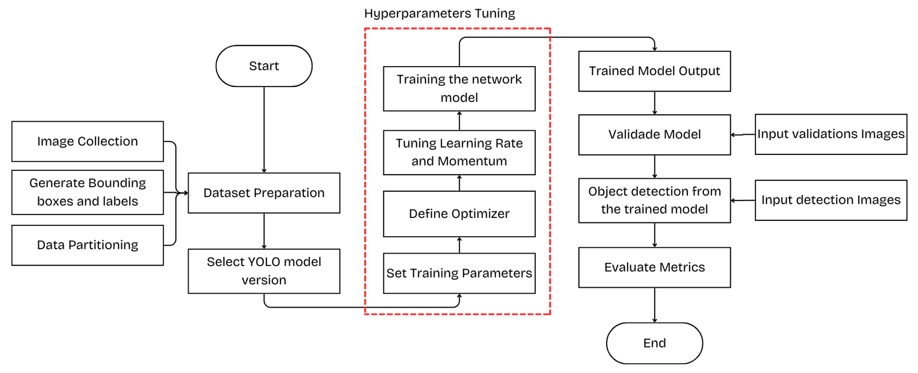
The first section of this article describes the concepts of architecture and the operation of the models used in the study. It also highlights the commonalities between YOLOv5, YOLOv8, and YOLOv11, detailing the evolution across these versions. Additionally, the section provides an overview of the hyperparameters and optimizers, emphasizing their role in optimizing the models used in this research. In the methodology section, the step-by-step process for extracting results is outlined, including key elements such as dataset creation, model training, model validation, and object detection using the trained models. Finally, the results section presents a comparison of the different simulation scenarios, allowing for an accurate assessment of the optimizations and adjustments applied during the study.

2. Literature Review

YOLO (You Only Look Once) is an object recognition architecture widely used in real-time detection scenarios. Its foundation is built on convolutional neural networks (CNNs), which represent image features in a manner that enables the precise identification and localization of objects within an image.

2.1. YOLOv5

Object detection architectures generally follow a common structure, which includes three key components: the Backbone, the Neck, and the Head. The Backbone is responsible for extracting features from the input image, compressing them using a feature extractor. The Neck (also known as the detection neck) aggregates these features, combining them to prepare for the final detection step. Finally, the Head (detection head) processes the aggregated features to identify and localize the objects within the image [15].

The YOLOv5 algorithm used in this work, in turn, has this architecture containing its three main parts:

The “Backbone”, a convolutional neural network structure which uses CSP-Darknet53. It has a topology of 53 convolutional layers and is based on the CSPNet architecture, ensuring a low computational cost [16,17].

The “Neck”, composed of an SPPF and CSP-PAN, which allow you to efficiently aggregate features and enable the CNN network to deal with inputs of variable size, without the need to resize or crop the original images [18].

The “Head” GIoU-loss, which is an evaluation metric commonly used in detecting objects. GIoU-loss consists of an extension of the IoU metric (Intersection over Union, Equation (1)) that takes into account the difference between the areas of the true and predicted bounding boxes [15].

$$IoU={\displaystyle \frac{(A\cap B)}{(A\cup B)}}$$

(1)

The GIoU loss, present in the Head of YOLOv5, is characterized by two arbitrary volumes $A,B\subseteq S\in {\mathbb{R}}^n$, and by the smallest space C that encompasses A and B, $C\subseteq S\in {\mathbb{R}}^n$. Equation (2) and Figure 1 demonstrate the calculation of GIoU, where C represents the smallest box that encloses A and B [19]:

$$GIoU=IoU={\displaystyle \frac{|C\setminus (A\cup B\left)\right|}{\left|C\right|}}$$

(2)

Figure 2 demonstrates a simplified example of the detection model used, in which the image is divided into S × S cells (grids) where each cell predicts the number of bounding boxes, where each box has its confidence value and its possibilities of belonging to a class of C objects, followed by the final detections delivered by the [20] algorithm.

2.2. YOLOv8

The eighth version of YOLO, released in January 2023, stands out for its superior performance in terms of both model accuracy and speed compared to previous versions. While its architecture remains similar to its predecessors, YOLOv8 retains the core components that define the YOLO framework: Backbone, Neck, and Head [21].

In this version, the Backbone continues to act as the feature extractor, while the Neck combines the extracted features, predicts object locations, and determines the object’s class [21].

One of the key innovations in YOLOv8 is the departure from anchor boxes, which were previously used to predict object locations and sizes. Unlike earlier versions, YOLOv8 adopts a model without anchors, directly predicting the center of an object. This change addresses challenges related to anchor boxes, such as poor generalization and difficulty handling irregular object shapes. It leads to a reduction in the number of predictions and improves the speed of the post-processing stage, which filters candidate detections after inference [6].

Another notable feature of YOLOv8 is its implementation of early stopping. This functionality automatically halts training when there are no improvements in the validation metric over a specified number of consecutive epochs. The patience parameter, which controls the number of epochs before stopping, can be adjusted as needed. For the simulations in this study, the default value of 50 epochs (patience = 50) was maintained.

In the present study, performance metrics were extracted from YOLOv5, YOLOv8, and YOLOv11, incorporating hyperparameter adjustments to assess improvements and provide a direct comparison between the models. The simulated hyperparameter values and the resulting performance comparisons will be discussed in the subsequent sections.

2.3. YOLOv11

YOLOv11 marks a new era in object detection in real time, bringing advances in precision, speed, and efficiency. This latest version, presented by Jocher and Qiu (2024), stands out for its enhanced architecture, which significantly improves feature extraction capabilities, and its optimized design, which effectively balances performance and computational cost. Compared to YOLOv8, YOLOv11 achieves higher mean average precision (mAP), making it ideal for applications on edge devices and cloud platforms. Furthermore, YOLOv11’s flexibility enables its application across a wide range of computer vision tasks, including object detection, instance segmentation, image classification, pose estimation, and oriented object detection (OBB) [22].

In comparison to its predecessors, YOLOv11 demonstrates a significant leap in balancing precision, speed, and computational efficiency. These advancements make it a prime candidate for deployment in real-time applications, ranging from autonomous vehicles to surveillance systems. Its adaptability across diverse hardware environments further underscores its practicality, catering to both resource-constrained edge devices and high-performance servers. By integrating state-of-the-art components like C2PSA and SPPF, YOLOv11 not only sets a new benchmark in object detection but also paves the way for further exploration in advanced computer vision tasks [23].

2.4. Hyperparameters

In general, hyperparameters are adjustable values that influence the model training process. They are not directly learned by the training algorithms, but can be adjusted before starting training. Their values directly impact the performance and effectiveness of the resulting model.

As highlighted by [8], several hyperparameters, such as input image size, number of epochs, batch size, learning rate, and momentum, can be tuned to optimize YOLO performance. Additionally, adjusting hyperparameters like the learning rate and momentum can significantly reduce training time and improve the model’s performance metrics.

2.5. SGD, Adam and AdamW Optimizers

When training convolutional neural networks for object detection, optimization algorithms play a crucial role. In the case of YOLOv5, YOLOv8, and YOLOv11, three distinct types of optimizers are employed: SGD (stochastic gradient descent), Adam (adaptive moment estimation), and AdamW (a variant of Adam). The choice of optimizer significantly influences the effectiveness of the model in object detection tasks [8].

SGD is a widely used optimization algorithm in machine learning and neural network training. By default, YOLO implementations use this optimizer in their codebase.

SGD calculates the gradient of the cost function with respect to the model parameters $\theta$ (the adjustable parameters of the neural network), as shown in Equation (3) below. The primary objective of SGD is to minimize the objective function $J\left(\theta \right)$, which represents the error or cost the model aims to reduce during training. The parameters $\theta \in {\mathbb{R}}^d$ are updated in the opposite direction of the gradient of $J\left(\theta \right)$, denoted as ${\nabla }_{\theta }J\left(\theta \right)$. The learning rate, $\eta$, controls the step size taken towards a local minimum. The parameter update rule for each training example, $x_i$, and its corresponding label, $y_i$, is given by Equation (4) below. In summary, SGD seeks to find the values of $\theta$ that minimize the objective function $J\left(\theta \right)$, thereby improving the model’s accuracy when evaluated against the training data [8].

$$\theta =\theta -\eta ·{\nabla }_{\theta }J\left(\theta \right)$$

(3)

$$\theta =\theta -\eta ·{\nabla }_{\theta }J(\theta ;x^i;y^i)$$

(4)

Both the Adam and AdamW optimizers build on the concepts of SGD but introduce adaptive learning rate adjustment techniques. These optimizers are used to adjust the network weights by calculating gradients, much like SGD. However, AdamW introduces weight regularization through weight decay, which generally leads to faster convergence to the optimal result.

Adam and AdamW are extensions of SGD, incorporating adaptive moment estimation. They calculate running averages of the gradients, denoted as $m_t$, and the squared gradients, denoted as $v_t$, as shown in Equations (5) and (6), respectively. These running averages represent the first and second moments of the gradients. The parameters are updated using the Adam rule, given in Equation (7). In this context, ${\beta }_1$ controls the exponential decay rate for the first moment estimate, ${\beta }_2$ controls the decay rate for the second moment estimate, and $g_t$ is the gradient calculated on the current batch of data. These elements are used to update $m_t$ and $v_t$ during the training process, ultimately leading to improved convergence in optimization [8].

$$m_t={\beta }_1{m}_{t-1}+(1-{\beta }_1)g_t$$

(5)

$$v_t={\beta }_2{v}_{t-1}+(1-{\beta }_2){g_t}^2$$

(6)

$${\theta }_t={\theta }_{t-1}-{\displaystyle \frac{\eta }{\sqrt{{\hat{v}}_t}}}+\epsilon +{\hat{m}}_t$$

(7)

3. Methodology

The research was conducted using the Google Colab tool, which offers an interactive notebook environment in the cloud, enabling code execution directly in the browser. The default environment includes Python 3, a T4 GPU hardware accelerator with 15 GB of GPU RAM, 12 GB of system RAM, and 80 GB of available storage.

In this context, Figure 3 illustrates the process followed, from the initial setup to the evaluation of the results. The first step involved creating a custom image bank for training. A database of 211 images was required to compare the performance of different models using the same dataset. The Roboflow platform was used to create and manage the image bank for model training, and the step-by-step process is described below.

Table 1. Characteristics of the image database used.

Database	Total	Training	Validation	Test
Dataset	211	157	32	22

outlines the characteristics of the image bank used in the training. The dataset consists of 211 images, with 75% designated for training, 15% for validation, and 10% for testing.

The dataset must follow a standard specific to the YOLO algorithm, where images for training, validation, and detection (testing) must be provided in separate folders. This configuration was carried out using Roboflow.

3.1. Creating a Dataset

To create the image bank, a selection of images featuring trees in various scenarios was made. These images were gathered from publicly available repositories on the internet. Once the 211 images were selected, labels were assigned to indicate which objects the model should learn to identify. This labeling process was carried out using the Roboflow tool, which involves defining regions within the images that represent a specific class— in this case, “tree”.

Each object is manually outlined with a rectangle, known as a bounding box, and its dimensions are provided in relation to the image, with boundaries described in text format. As a result, each image is accompanied by two files: the image itself in .JPG format, and a .txt file containing the coordinates of each bounding box that represents a tree in the image. This text file is referred to as the Labels file. An example of this process is shown in Figure 4.

For this example, two bounding boxes were created to represent the “tree” class. Along with the image, a .txt file is generated, where the first number indicates the class, and the subsequent numbers represent the coordinates of the bounding box, as shown in Figure 5. Each line in this file corresponds to a delimited object within the image, with the second number in each line representing class 0 (tree).

Once the bounding boxes were defined, the dataset was exported, and the model to be used was selected. At this stage, the proportions and quantities of images required for each phase of the training process (training, validation, and testing) were also determined.

3.2. Model Training

For training the model, the following parameters were used:

-

img 640: This parameter specifies the size of the images during training. In this case, the images are resized to 640 × 640 pixels.

-

batch 16: This refers to the batch size, or the number of images that will be processed in parallel during each training iteration.

-

epochs 100: This command defines the number of training epochs, meaning the number of times the algorithm will process the entire training dataset.

-

yolov5s.pt: YOLOv5 offers pre-trained models that can be selected in advance. For this study, the smallest and fastest model, YOLOv5s, was used, as it is considered optimal for speed and performance according to its documentation [21].

Following the same application as YOLOv5, we use the configurations that the YOLOv8s and YOLOv11s models bring, maintaining the standards when carrying out the training, and varying the model between 5, 8 and 11.

Furthermore, it was necessary to define the hyperparameters, create text files containing these settings, and modify the initial learning rate (lr0) and momentum (m) values. The variations in hyperparameters are shown in

Table 2. Values of the hyperparameters used for each training with each optimizer.

Learning Rate	Momentum
0.01	0.937
0.001	0.9
0.001	0.99
0.001	0.999
0.0001	0.9
0.0001	0.99
0.0001	0.999

. It is important to note that these values were applied consistently across the three optimizers (SGD, Adam, and AdamW) and for all three models (YOLOv5, YOLOv8, and YOLOv11).

3.3. Model Validation

The validation process involves using the “weights” generated during training to extract metrics and assess the performance of the trained model. At this stage, images that were not part of the training set are used.

During validation, model accuracy, recall, and precision curves are generated. Additionally, object detection results are evaluated, as shown in Figure 6. For this study, specific comparative values were used, which will be discussed in detail in the results section of this article.

3.4. Object Detection from the Trained Model

The detection process is the stage where the model’s training is put to the test. For this step, the “test” set of images was used, which consisted of completely different images from those used in the training and validation phases.

The outcome of this stage is an image with the detected object and its associated accuracy rate. In other words, it shows the model’s confidence level in the detection, as illustrated in Figure 7.

4. Results and Discussion

After the training carried out, important metrics were obtained to evaluate the results of the model obtained.

Among the metrics extracted, precision is observed, which is equivalent to the measurement of the proportion of positive examples correctly identified in relation to the sum of true positives and false positives. In other words, an accuracy of 1 indicates that all examples identified as positive by the model are really positive; therefore, there are no false positives. A precision of 0 represents that all examples identified as positive by the model are negative; that is, they are all false positives.

The recall graph evaluates the proportion of positive examples that were correctly identified by the model in relation to the total number of positive examples in the data set. Thus, a recall of 1 means that the model correctly identified all positive examples, with no false negatives. On the other hand, a recall of 0 represents that the model was unable to identify any positive examples, with only false negatives.

Thus, with the precision and recall values, it becomes possible to calculate the average precision, the mAP (mean average precision). As presented in [24], the mAP, precision (P) and recall (R) are initially calculated:

$$P={\displaystyle \frac{TP}{TP+FP}}$$

(8)

$$R={\displaystyle \frac{TP}{TP+FN}}$$

(9)

where:

• TP (true positive) represents the number of samples whose labels are positive, meaning the true predictions are positive;
• FP (false positive) indicates the number of samples whose labels are negative, meaning the real predictions are positive;
• FN (false negative) represents the number of samples whose labels are positive, meaning the real predictions are negative (not detected).

Therefore, the mAP represents the average of different APs, where AP represents the area under the PR curve. The mAP is calculated as follows:

$$mAP={\displaystyle \frac{1}{K}}\sum _{i=1}^K(R_i-R_{i-1})P_i$$

(10)

where K represents the number of categories, R is recall, and P is precision.

The F1 score is a widely used metric in the evaluation of object detection models, particularly for adjusting the balance between precision and recall. Precision is related to the model’s ability to correctly identify objects present in an image, while recall is associated with the model’s ability to detect all objects, including those that may be more difficult to identify. However, there is a trade-off between these two metrics, where an increase in precision typically results in a decrease in recall, and vice versa. The F1 score, which represents the harmonic mean between precision and recall, is an effective metric for evaluating the performance of object detection models, as it takes into account both precision and recall in a balanced way [8,25,26].

$$F1Score=2\ast {\displaystyle \frac{Precision\ast Recall}{Precision+Recall}}$$

(11)

This mAP value is represented over a specific range of confidence values. That is, the detection is considered correct if the model confidence is equal to or greater than the mAP value. In this case, YOLOv5, YOLOv8, and YOLOv11 provide two types of data and graphs: one with a confidence interval greater than 0.5, and another with values ranging between 0.5 and 0.95

Next, the values obtained after validating the trained model will be demonstrated, consisting of precision values, recall, mAP50, mAP50-95. This is carried out, initially for YOLOv5 and later for YOLOv8 and YOLOv11, using an image bank composed of 211 images, created specifically by the author in this study.

The different training scenarios can be seen in

Table 3. Results of training with hyperparameter variation, using the SGD optimizer and YOLOv5.

Learning Rate	Momentum	Precision	Recall	mAP50	mAP50-95	F1 Score
0.01	0.937	0.955	0.84	0.902	0.641	0.894
0.001	0.9	0.908	0.776	0.865	0.586	0.836
0.001	0.99	0.89	0.791	0.879	0.625	0.836
0.001	0.999	0.864	0.872	0.877	0.623	0.868
0.0001	0.9	0.332	0.314	0.311	0.103	0.323
0.0001	0.99	0.881	0.686	0.761	0.476	0.772
0.0001	0.999	0.888	0.667	0.76	0.494	0.765

and

Table 4. Results of training with hyperparameter variation, using the Adam optimizer and YOLOv5.

Learning Rate	Momentum	Precision	Recall	mAP50	mAP50-95	F1 Score
0.01	0.937	0.905	0.863	0.920	0.586	0.884
0.001	0.9	0.916	0.882	0.919	0.646	0.899
0.001	0.99	0.881	0.824	0.884	0.575	0.852
0.001	0.999	0.841	0.745	0.842	0.555	0.791
0.0001	0.9	0.879	0.843	0.846	0.575	0.860
0.0001	0.99	0.824	0.843	0.869	0.555	0.833
0.0001	0.999	0.970	0.725	0.842	0.515	0.826

. Thus, for each table, the highest values for each extracted metric have been highlighted. It is worth mentioning that the first case in each table relates to the standard values brought by the YOLOv5 algorithm, with values of 0.01 and 0.937, for the learning rate and momentum, respectively.

As shown in Table 3, for example, it is noted that when using the SGD optimizer with YOLOv5, the configuration that achieved the highest precison and recall values for the model was obtained by adjusting the hyperparameters with a learning rate of 0.001 and a momentum of 0.999, producing values of 0.864 and 0.872, respectively. This indicated an improvement in performance in terms of correctly identifying positive examples, thereby reducing the false positive rate in the results.

Meanwhile, the F1 score values calculated for the different configurations show that although variations in the learning rate and momentum significantly impact the model’s performance, the F1 score provides a comprehensive view of overall effectiveness, considering both precision and recall. In the case of a configuration with a learning rate of 0.001 and momentum of 0.999, the F1 score of 0.868 reflects a good balance between precision and recall, indicating that the model was able to maintain a solid equilibrium between true positives and the identification of all relevant instances.

Table 4 presents the scenario with the Adam optimizer, where an improvement in the recall (0.882) and mAP50-95 (0.646) metrics was observed when using hyperparameters with values of 0.001 and 0.9. The best precision scenario, 0.97, was achieved by adjusting the learning rate and momentum parameters to 0.0001 and 0.999, respectively. Therefore, it can be concluded that hyperparameter adjustments, in these scenarios, lead to improvements in both precision and confidence intervals in image detection, as evidenced by the increase in mAP, which reached 0.646 for mAP50-95 and 0.920 for mAP50.

The hyperparameter adjustment, lr = 0.0001 and m = 0.999, also resulted in an F1 score of 0.826. This configuration stood out for its balance between precision (0.970) and recall (0.725), reflecting robust and optimized performance, indicating a significant improvement in results, and showing that a lower learning rate contributed to higher precision in training.

Finally, when using the AdamW optimizer, improvements were observed by adjusting the parameters to 0.001 and 0.9. In this scenario, the model demonstrated better precision (0.916) and a higher mAP rate (0.916 and 0.657), as presented in

Table 5. Results of training with hyperparameter variation, using the AdamW optimizer and YOLOv5.

Learning Rate	Momentum	Precision	Recall	mAP50	mAP50-95	F1 Score
0.01	0.937	0.891	0.843	0.890	0.594	0.866
0.001	0.9	0.916	0.860	0.916	0.657	0.888
0.001	0.99	0.904	0.804	0.876	0.583	0.852
0.001	0.999	0.802	0.804	0.851	0.551	0.803
0.0001	0.9	0.864	0.875	0.878	0.599	0.869
0.0001	0.99	0.854	0.804	0.867	0.554	0.828
0.0001	0.999	0.815	0.765	0.819	0.494	0.790

. In this way, the best result presented by the YOLOv5 model in terms of mAP50-95 stands out, representing the scenario with the highest confidence interval in detection, where its value reached 0.657.

In this table, the best F1 score values are also observed with the combination of learning rate = 0.001 and momentum = 0.9, with an F1 score of 0.888. This value stands out not only for its superior precision and recall but also for providing a significant gain compared to other configurations, reflecting a good balance between the learning rate and momentum. The variation in momentum, especially for higher values like 0.99 and 0.999, did not bring considerable improvements, suggesting that a more balanced choice of 0.9 is more effective.

As shown in

Table 6. Results of training with hyperparameter variation, using the SGD optimizer and YOLOv8.

Learning Rate	Momentum	Precision	Recall	mAP50	mAP50-95	F1-Score
0.01	0.937	0.950	0.804	0.888	0.657	0.869
0.001	0.9	0.973	0.804	0.928	0.676	0.878
0.001	0.99	0.932	0.811	0.893	0.662	0.869
0.001	0.999	0.913	0.804	0.913	0.693	0.856
0.0001	0.9	0.787	0.797	0.821	0.591	0.792
0.0001	0.99	0.935	0.882	0.931	0.646	0.908
0.0001	0.999	0.900	0.881	0.936	0.665	0.890

, the use of YOLOv8 with the SGD optimizer and the variation of the hyperparameter with the selected values is evident. In this context, the value that brought the highest precision (0.973) to the model was achieved by adjusting the hyperparameters to have a learning rate of 0.001 and a momentum of 0.9.

Another important aspect to highlight in this scenario is that a learning rate of 0.0001 and a momentum of 0.999 were associated with the highest average mAP (0.936), indicating a greater number of cases where object detection had a confidence rate above 50%. Furthermore, using hyperparameter values of 0.001 and 0.999, the best result was obtained for the confidence interval between 50% and 95% in mean mAP (0.693).

In the case of the SGD optimizer and YOLOv8, the best F1 score value was achieved with a learning rate = 0.0001 and momentum = 0.99, with an F1 score of 0.908. This value is remarkable because it reflects an excellent balance between precision and recall, with an impressive recovery for higher momentum values. Although the model with learning rate = 0.001 and momentum = 0.9 achieved higher precision (0.973), its performance in recall and F1 score of 0.878 was not surpassed. The improvement in F1 score across the different learning rate combinations also emphasizes the importance of optimally adjusted hyperparameters.

The training results using the Adam optimizer and YOLOv8 can be seen in

Table 7. Results of training with hyperparameter variation, using the Adam optimizer and YOLOv8.

Learning Rate	Momentum	Precision	Recall	mAP50	mAP50-95	F1 Score
0.01	0.937	0.798	0.774	0.849	0.590	0.786
0.001	0.9	0.907	0.804	0.914	0.688	0.854
0.001	0.99	1.0	0.842	0.883	0.659	0.912
0.001	0.999	0.922	0.784	0.908	0.650	0.850
0.0001	0.9	0.958	0.893	0.931	0.697	0.924
0.0001	0.99	0.956	0.859	0.928	0.669	0.906
0.0001	0.999	0.932	0.863	0.900	0.667	0.897

, and they demonstrate that, out of all the configurations, this one achieved the best result in terms of precision. With a precision value of 1.00 for a learning rate of 0.001 and momentum of 0.99, it indicates that all examples identified as positive by the model are indeed positive. Therefore, there are no false positives in this case.

Additionally, another notable scenario used values of learning rate = 0.0001 and momentum = 0.9, which led to an improvement in results related to recall (0.893) and an average mAP of 0.931 and 0.697.

In the table with Adam and YOLOv8, the best performance was also achieved for the F1 score with a learning rate = 0.0001 and momentum = 0.9, reaching a value of the F1 score of 0.924. This value stood out due to the optimized balance between precision (0.902) and recall (0.882), providing an excellent combination of object detection capability and minimization of false negatives. The significant improvement in F1 score with this configuration reflects a considerable gain compared to other hyperparameter combinations. The choice of a lower learning rate with momentum = 0.9 appears to be one of the main contributors to this strong performance. The high precision value, compared to other momentum combinations, further highlights the model’s ability to correctly classify objects.

The results in

Table 8. Results of training with hyperparameter variation, using the AdamW optimizer and YOLOv8.

Learning Rate	Momentum	Precision	Recall	mAP50	mAP50-95	F1 Score
0.01	0.937	0.829	0.858	0.870	0.600	0.843
0.001	0.9	0.854	0.915	0.933	0.674	0.884
0.001	0.99	0.910	0.795	0.912	0.658	0.849
0.001	0.999	0.968	0.784	0.876	0.653	0.858
0.0001	0.9	0.902	0.882	0.956	0.707	0.892
0.0001	0.99	0.895	0.840	0.916	0.688	0.866
0.0001	0.999	0.940	0.843	0.918	0.675	0.889

demonstrated an improvement when using the parameters 0.001 and 0.9 for the learning rate and momentum. In this case, the best scenario for recall (0.915) is highlighted, where the model correctly identified a larger number of positive examples, resulting in fewer false negatives. The scenario with the best mAP index (0.956) was also achieved using the AdamW optimizer, but with learning rate values of 0.0001 and momentum values of 0.9. For precision (0.968), the improvement was notable when using learning rate = 0.001 and momentum = 0.999.

The highest F1 score was recorded with learning rate = 0.0001 and momentum = 0.9, with an F1 score of 0.892. The improvement in F1 score is significant compared to the other hyperparameters, especially considering that the model with learning rate = 0.0001 and momentum = 0.999 achieved only a slightly lower performance (0.889). The increase in F1 score when using momentum = 0.9 instead of higher values, such as 0.99 and 0.999, suggests that more subtle adjustments to this parameter can lead to substantial improvements. The improvement in F1 score reflects not only an increase in precision but also a significant recovery in terms of recall, resulting in a very efficient overall combination.

Table 9. Results of training with hyperparameter variation using the SGD optimizer and YOLOv11.

Learning Rate	Momentum	Precision	Recall	mAP50	mAP50-95	F1 Score
0.01	0.937	0.968	0.784	0.905	0.658	0.866
0.001	0.9	1.000	0.862	0.934	0.674	0.926
0.001	0.99	0.952	0.784	0.909	0.704	0.860
0.001	0.999	0.977	0.784	0.914	0.659	0.870
0.0001	0.9	0.870	0.790	0.868	0.607	0.828
0.0001	0.99	0.937	0.879	0.936	0.683	0.907
0.0001	0.999	0.919	0.894	0.952	0.689	0.906

presents an analysis of the impact of hyperparameter adjustments during the training of the YOLOv11 model using the SGD optimizer. Among the configurations evaluated, the combination of a learning rate of 0.001 and a momentum of 0.9 achieved the highest performance in terms of precision (1.000) and F1 score (0.926). However, in terms of the average mAP50 and mAP50-95 metrics, the configuration with a learning rate of 0.0001 and a momentum of 0.999 proved to be more effective (0.952 and 0.689). These results highlight that different objectives can be achieved through specific hyperparameter adjustments, emphasizing the importance of careful calibration to optimize the model’s overall performance according to the training priorities.

Table 10. Results of training with hyperparameter variation using the Adam optimizer and YOLOv11.

Learning Rate	Momentum	Precision	Recall	mAP50	mAP50-95	F1 Score
0.01	0.937	0.865	0.754	0.832	0.598	0.806
0.001	0.9	0.976	0.802	0.897	0.688	0.880
0.001	0.99	0.930	0.776	0.888	0.645	0.846
0.001	0.999	0.926	0.824	0.884	0.633	0.872
0.0001	0.9	0.922	0.784	0.917	0.706	0.847
0.0001	0.99	0.933	0.822	0.932	0.704	0.874
0.0001	0.999	0.914	0.863	0.926	0.684	0.888

presents the hyperparameter adjustments using the Adam optimizer, highlighting significant improvements in accuracy across all simulated scenarios. Notably, the case where the learning rate was adjusted to 0.001 achieved an accuracy of 0.976 and a balance between precision and recall, as demonstrated by the F1 score of 0.880. Additionally, by adjusting the hyperparameters to a learning rate of 0.0001 and momentum of 0.999, the trained model showed remarkable evolution in terms of recall (0.863), mAP50 (0.926), and mAP50-90 (0.684).

In the case of the AdamW optimizer applied to the YOLOv11 model, as indicated in

Table 11. Results of training with hyperparameter variation using the AdamW optimizer and YOLOv11.

Learning Rate	Momentum	Precision	Recall	mAP50	mAP50-95	F1 Score
0.01	0.937	0.878	0.765	0.844	0.631	0.818
0.001	0.9	0.968	0.843	0.930	0.677	0.901
0.001	0.99	0.898	0.859	0.896	0.654	0.878
0.001	0.999	0.858	0.843	0.867	0.631	0.850
0.0001	0.9	0.933	0.814	0.918	0.702	0.869
0.0001	0.99	0.954	0.816	0.896	0.691	0.880
0.0001	0.999	0.953	0.800	0.912	0.673	0.870

, significant advancements in the evaluated metrics were observed. The most prominent scenario occurred when the learning rate was set to 0.001 and momentum to 0.9, where the model achieved an accuracy of 0.968, recall of 0.843, mAP50 of 0.930, and F1 score of 0.901. It is worth noting that in the other analyzed scenarios, improvements were also observed in all metrics, with consistently higher values than the standard benchmarks. In particular, the accuracies and mAP50 indices exceeded 0.9 in most cases of hyperparameter adjustment.

Next, we observe the evolution of the mAP indices throughout the model iterations, for each hyperparameter adjustment performed with each optimizer and for YOLOv5, YOLOv8, and YOLOv11 models.

Figure 8, Figure 9, Figure 10, Figure 11, Figure 12, Figure 13, Figure 14, Figure 15 and Figure 16 show the evolution of this metric, where each line in the graph represents a combination of hyperparameters composed of a learning rate (lr) and momentum (m). Furthermore, it is worth highlighting that each figure corresponds to an optimizer used, i.e., SGD, Adam, or AdamW for a given model, be it YOLOv5, YOLOv8, or YOLOv11.

In Figure 8, it is shown that the best case for an mAP:50 effectively occurred when using the default value of lr = 0.01 and m = 0.937. It is also observed that some cases maintained behavior very close to the standard, without significant gains, while others had a decline in performance, bringing values below the standard.

When using the Adam optimizer in conjunction with YOLOv5, positive gains were obtained when adjusting the hyperparameters to lr = 0.001 and m = 0.9. As shown in Figure 9, the curve that represents the model’s behavior, with these values converging to its value far more rapidly. It is also observed that around the time 60, the curve already becomes more constant, meaning that there are no longer significant improvements in the validation metric for a specified number of consecutive epochs. With the standard values, the curve takes longer to converge, occurring only from the 90s onwards, proving a gain in performance and speed when reaching these values.

Similarly, an improvement is observed when reaching the mAP metrics in Figure 10, through faster convergence to its final value. In this scenario, the best mAP value also stands out for lr = 0.001 and m = 0.9. Another positive result is for cases in which lr = 0.001 and momentum vary with values of 0.99 and 0.999, as in these cases, the values were also reached more quickly compared to the standard.

These same scenarios were also replicated in YOLOv8, as represented in Figure 11, Figure 12 and Figure 13, in which we have the result of the behavior when generating the mAP50 metrics.

For the SGD, the hyperparameters that best generated an average mAP50 were the values of lr = 0.0001 and momentum = 0.999. In addition to being the best value scenario, it is a quick approximation of the final value. From the 60th epoch onwards, a value closer to the end was already obtained, unlike the standard case, which presented a lower performance characterized by large variations in its mAP value until approximately the 80th epoch. All other scenarios with different hyperparameter values had a good result, with similar behavior between them and a close average value, with the exception of the case where lr = 0.0001 and momentum = 0.9, which performed poorly. Figure 11 exemplifies these results.

When using Adam as an optimizer for YOLOv8, the case that stood out the most was using hyperparameters lr = 0.0001 and momentum = 0.9, in which it presented the highest value of mAP50. At this stage, good behavior stands out for all curves referring to lr = 0.0001. Even with momentum 0.9, 0.99 or 0.99, the model converged to a good mAP value of close to 0.900. An advantage observed when using momentum = 0.999 was a case of early stopping, in which around the 80th epoch, the model had already stabilized without presenting significant changes in the metric values, thus ending the simulation early. This reinforces a performance gain in this case (Figure 12).

For the AdamW optimizer applied to YOLOv8, the worst performance case was obtained with the default values, proving the gain when adjusting the hyperparameters. For the best case, we have lr = 0.0001 and m = 0.9. A peculiarity of YOLOv8 is the early stopping, which can be seen in the following graph, as from the 80th iteration executed (epoch) onwards, there were no significant gains in improving metrics. Therefore, the model automatically terminates the process. In this way, you obtain a much faster result, as you have identified that it would no longer be necessary to carry out further iterations, as you have reached your best value. Also noteworthy is the behavior of other values, which, in turn, converge quickly, being faster than the standard case (Figure 13).

Regarding the evolution of the mAP50 metric using SGD and YOLOv11, as illustrated in Figure 14, a consistent improvement in model performance was observed when applying the combination of a learning rate of 0.0001 and a momentum of 0.999. This configuration resulted in higher mAP50 values and exhibited a faster convergence to the maximum value, highlighting the effectiveness of hyperparameter adjustments. In contrast, the default configuration, with a learning rate of 0.01 and a momentum of 0.973, showed frequent oscillations, a longer convergence time, and lower values compared to the other configurations.

Regarding the evolution of mAP50 when using the Adam optimizer and the YOLOv11 model, as illustrated in Figure 15, it is observed that hyperparameter adjustments resulted in significant improvements. All curves reach higher values and converge more quickly compared to the standard settings (lr = 0.001 and m = 0.937). The best scenarios are highlighted, where the mAP50 metric exceeded 0.9 when using combinations of lr and momentum such as 0.001 and 0.99, 0.0001 and 0.99, and 0.0001 and 0.999. These results demonstrate that lower learning rate values and higher momentum values yield better performances for this model.

Finally, Figure 16 shows the evolution of mAP50 for the AdamW optimizer applied to the YOLOv1 model. This case also highlights the model’s improvement with hyperparameter adjustments, as once again, the curves corresponding to the adjusted learning rate and momentum values outperform the standard curve.

5. Conclusions

This study implemented improvements in the performance of YOLO models in tree detection through the optimization of hyperparameters combined with the SGD, Adam, and AdamW optimizers. When comparing the different scenarios, the adjustments to these parameters actually brought improvements in relation to precision, recall, F1 score, and average mAP.

Regarding YOlOv5, when using AdamW together with learning rate = 0.001 and momentum, it resulted in the highest mAP index, with values of 0.916 for mAP50 and 0.657 for mAP50-95, in the general context. We also noted gains in precision and recall for all simulated cases, in addition to the improvement in the speed with which the mAP graphs converge to the metric value, as presented in the discussion.

In the YOLOv8 model, improvements were observed across all metrics, with emphasis on the case where the Adam optimizer was used with a learning rate of 0.0001 and momentum of 0.9, achieving precision of 95.8%, recall of 89.3%, mAP50 of 93.31%, mAP50:95 of 69.7%, and an F1 score of 92.4%. Additionally, AdamW demonstrated effectiveness with configurations of learning rate = 0.0001 and momentum = 0.9, as well as learning rate = 0.0001 and momentum = 0.999, where early stopping occurred due to metric values stabilizing without significant changes. These AdamW configurations yielded higher mAP50 values (0.956 and 0.918), further validating the performance gains achieved through the implemented changes.

Regarding the latest YOLOv11 version, the improvements obtained through hyperparameter adjustments were observed in the majority of simulated scenarios. The model demonstrated higher accuracy metrics compared to standard configurations when using SGD. Specifically, it achieved a precision of 1.000 with a learning rate (lr) of 0.001 and momentum (m) of 0.9, and 0.977 for lr = 0.001 and m = 0.999. The most notable case occurred with lr = 0.0001 and m = 0.999, achieving a recall of 0.894, mAP50 of 0.952, mAP50:95 of 0.689, and an F1 score of 0.906.

When using the ADAM optimizer, the best results for recall (0.863), mAP50 (0.932), mAP50:95 (0.706), and F1 score (0.888) were achieved with a learning rate of 0.0001 and momentum values ranging from 0.9 to 0.999. The highest precision value (0.976) was obtained with a learning rate of 0.001 and momentum (m) of 0.9. These findings demonstrate that combining a reduced learning rate with appropriate momentum values can maximize the model’s performance across the evaluated metrics.

For the configuration using the AdamW optimizer with YOLOv11, the highest precision values (0.968), recall (0.843), mAP50 (0.930), mAP50:95 (0.677), and F1 score (0.901) were obtained with a learning rate of 0.001 and a momentum of 0.9. This configuration highlights that a moderate learning rate combined with well-tuned momentum can offer superior performance by ensuring effective model training. Furthermore, AdamW’s weight regularization improvements significantly contributed to the improvement in performance metrics.

In fact, more effective values were observed in relation to YOLOv11 when compared to YOLOv5 and YOLOv8, but it was also concluded that when adjusting the hyperparameters combined with different optimizers, they became effective for all and gave better results and metrics. The performances of YOLOv5, YOLOv8, and YOLOv11 were satisfactory when identifying trees in a non-standard image bank, and the present study presented the behavior of each model so that, in future applications, they can assist in decision-making when implementing the algorithm in an application.