Standards for the Weighting of Criteria and the Measurement of Interaction

Abstract

This article discusses the need for standards for the assignment of importance to criteria and the measurement of interaction between them in multiple criteria analyses of complex systems. A strategy for criteria evaluation is considered that is suitable to account for the interaction among a wide variety of imprecisely assessed criteria applied simultaneously. It is based on the results of collecting sample information on preferences according to the specified criteria instead of merely an abstract comparison of the criteria. The comparison of alternatives is based on objectives that determine the formation of preferences. It is facilitated by a rating in terms of preference probabilities. Probabilistic standards grant homogeneity of measurements by different criteria, which is useful for the combination of the criteria. These standards apply to a sampling evaluation conducted via pairwise trichotomic comparison of the alternatives according to each criterion, followed by the combination of these multiple evaluations into a single global score by means of the Choquet Integral with respect to a capacity determined by applying preference concentration to the sets of probabilistic assessments. Examples of practical application are discussed.

1. Introduction

The main motivation for this study comes from the need for standards for the assignment of importance to criteria and for the modeling of the interactions between them in a multiple criteria decision analysis (MCDA) dealing with a large variety of criteria subject to random disturbances and interacting with each other. The abundance of distinct methods in the field [1,2] makes the search for such standards more relevant. Standards streamline decisions, for instance, in situations such as making an emergency health decision [3], facing a sudden enemy military attack [4], offering advice regarding stock trading under volatile market conditions [5], or choosing a supplier for a failing critical component [6].

Another aspect of situations that makes the establishment of standards important is the complexity and subjectivity of the application of the related criteria [7,8]. As a consequence, it is important not only to simplify the measurements but also to make them comparable and to ensure that the relations between the measurements according to different criteria, the forms of criteria importance assessment, and the criteria combination rules can be easily explained. In these situations, combining a large variety of criteria, avoiding arbitrarily assigning unequal importance to them, and accounting for the complexity of their relations necessitates a set of simple and well-defined standards governing the key analysis procedures.

One situation involving complex and subjective decisions is that of the prediction of electoral preferences. Electoral preference prediction models can be classified into two categories: fundamental models and polling models. Fundamental models attempt to derive votes from economic and social explanatory variables. Polling models address only the final voting preferences. They pose the single question: “if the election were today, who would you vote for?”

Due to a low predictive power observed in the models of the first category, the currently prevailing models tend to combine variables from poll models with other variables, which mostly serve to evaluate the personal qualities of the candidates or the approval of parties’ incumbents [9,10,11]. Formulating the choice in terms of individual preferences regarding individual qualities strengthens individualistic motives.

Behind such an assessment model for individuals is the rational choice assumption that the members of the sample weigh their reasons mentally. In contrast, by making explicit the multiple objectives that interact in the formation of personal preference, complex MCDA models emphasize these objectives themselves. In an assessment of the preferences of the population, this has the effect of strengthening the pursuit of the common good. To project a long-term goal, a nation must have it as a collective target.

Collective objectives that lose importance in the modeling of preferences also lose importance in the culture in which those preferences are formed. In contrast, the modeling of preferences based on matters of collective interest will favor the prevalence of a culture of collaboration around collective goals. If elicited in preference assessments, the positioning with respect to civil rights, the size of the government, environmental protection, development goals, and other objectives of high importance will, in turn, be more present in the political scenery.

In recent years, modern economic growth theory has shifted from the classical theory emphasizing capital and labor productivity to a theory emphasizing the roots of productivity in the form of ideas and institutions [12]. Countries that are open to ideas invest in education and create efficient institutions. The predictions based on economic and social objectives supply the motivation for these efforts.

From a parsimony perspective, a small number of variables with high predictive power for certain aspects of the decision can make a prediction model more efficient. To become competitive, models encompassing a large set of interacting variables must be supported by efficient fitting strategies.

The standard procedures in MCDA provide for the safe consideration of a large number of objectives that drive the choice of a model. These standards should be simple but comprehensive to allow for models that capture the complexity of the reality to be addressed.

The development of such standards is, then, an important research issue, and the lack of a reliable set of standards constitutes a serious gap in the MCDA research area. The present study fills this gap.

Here, standards for combining preferences established by multiple criteria whose importance is derived from their ability to identify the most preferred alternatives are discussed. Included are standards for the comparison of alternatives according to each criterion [13,14], standards for the combination of evaluations based on separate criteria into a global score [15,16], and standards for the measurement of the importance of interacting criteria [17,18,19]. The development of an analysis applying these standards will always serve as a basis for the comparison of the results of the application, in every case, of any MCDA method recommended by the peculiarities of the case.

The article is structured as follows. After this introduction, Section 2 sets the foundations for establishing standards for data collection, criteria comparison, and evaluations combination. Desirable properties of the decision rules are then established. Section 3 deals with the application of the principles and procedures advanced in the preceding section. Section 4 discusses the results obtained in Section 3 based on the analysis of practical situations. A set of conclusions on the viability and the usefulness of the standards established is presented in Section 5.

2. Materials and Methods

To be able to account for a wide variety of criteria, the assessment of preferences must be simple. By reducing the opportunities for the occurrence of errors in the measurement, simplicity engenders reliability.

Another important quality is comparability. To combine preferences among the alternatives being evaluated according to diverse criteria to obtain global scores, it is necessary to determine measurement standards that make the preferences assessed comparable in accordance with the different criteria.

An even more fundamental feature is representativeness. Alternatives must be evaluated based on their degree of commitment to an objective that is considered relevant to sustaining a criterion. How can such degrees of commitment be measured in a simple and comparable form?

The sampling of pairwise trichotomic comparisons exhibits all the desired properties. This assessment standard consists of assessing a sample of randomly selected representatives, either of the population or of experts, to determine, for every pair of alternatives, whether each of them is more capable than the other of reaching the desired objective. In the case of a tie, the preference measure is equal for both.

The small number of possible values, namely three, enhances robustness [20,21]. For instance, if, in a more detailed preliminary assessment, a distorted “very high” preference classification is given to one alternative, this alternative shares, in the comparison with an alternative with a “small” initial evaluation, the same preference assessment with any other alternative with a “high” classification.

If different scales of measurement of a single attribute have different meanings for different objectives, this same attribute may be used in different criteria with different roughness [22,23]. For instance, a complementary criterion can be built by imposing a transitivity requirement on experts’ ratings to tie more pairs of alternatives.

In the same sense, if considering more precise distances between alternatives is found to be useful, additional criteria can be created to represent narrower levels of variance. For instance, in a first criterion, two alternatives may be considered equivalent if the difference between their values in a certain attribute is smaller than 10, whereas, in a second criterion, they may be considered equivalent only if the difference is smaller than 1.

Counting the number of pairs exhibiting a preference for each alternative serves as the basis for calculating preference probabilities. Shifting from attribute measures to probabilities of preference has the benefit of unifying all evaluations to the same scale of measurement. This property of the commensurability is an essential condition to enable the combination of the criteria by means of the Choquet Integral [24].

From assessments of preference based on diverse criteria, we need to move to a measure of preference that considers all the criteria collectively. Counting favorable cases in pairwise trichotomic comparisons may still be useful to measure joint preference. However, this count does not consider the interactions between criteria. For such a calculation, the Choquet Integral of the preference probabilities according to each criterion is the simplest form. It will be calculated with respect to a capacity designed to adequately measure the relevance of each criterion considering their interactions.

The principle of concentration of preferences [19] makes it possible to derive such capacity. This principle, consistent with aversion to uncertainty in the decision-making process, leads a decision-maker to seek the maximization of the ability to discriminate the most preferred alternative. It leads, in the case of determining capacities of sets of criteria, to assign greater importance to those sets that exhibit a higher ability to point to an alternative as the most preferred. The importance of criteria is related to the personal aim of the decision-maker to choose the best among the available alternatives, and, barring possible gross mistakes, high measurements provide more reliable information about differences in preference than low measurements do.

Assuming an absence of interaction, the principle of preference concentration allows for the use of weighted averages with weights indirectly extracted from the results of the application of the criteria to the alternatives. In this case, the weights will be proportional to the maximal probabilities. However, by allowing for interaction, the combination via the Choquet Integral provides a more general standard. In the opposite direction, assumptions of generalized additive independence and other forms of modeling relations among criteria [25] are even less restrictive, but, compared to such approaches, the Choquet Integral has the advantage of simplicity.

When interaction is assumed to be absent and weighting average of the preference probabilities for isolated criteria is performed, the global preferences still add to 1, while, when the preferences are combined via the Choquet Integral with respect to a nonadditive capacity, this sum can vary. Nevertheless, the possibility of interaction being present must always be considered.

When pairs of criteria are evaluated, instead of isolated criteria, if two criteria agree in giving high preference to an alternative, even if it is not the most preferred by either of them, their high joint preference for this alternative results in a high capacity for the union of the two corresponding unitary sets. The capacities of sets of more than two criteria are determined similarly.

Why does this construction suitably consider interactions? Interaction is present in the selection process if a choice of an alternative according to a given criterion either increases or decreases the effect of the preference according to other criteria. A preference criterion interacts with others in the selection of the best alternative if its inclusion in addition to the others in the evaluation process increases or reduces the probability that the best alternative will be identified.

The same applies to groups of criteria regardless of the reason for the influence. Such reasons may include exchangeability, complementarity, substitutability, or preferential dependence [26], but only the effect, not the origin, of the interaction needs to be established.

This application of the principle of preference concentration is similar to maximum likelihood estimation. It attributes to a criterion a capacity proportional to the preference value that this criterion assigns to the alternative to which it assigns the highest preference.

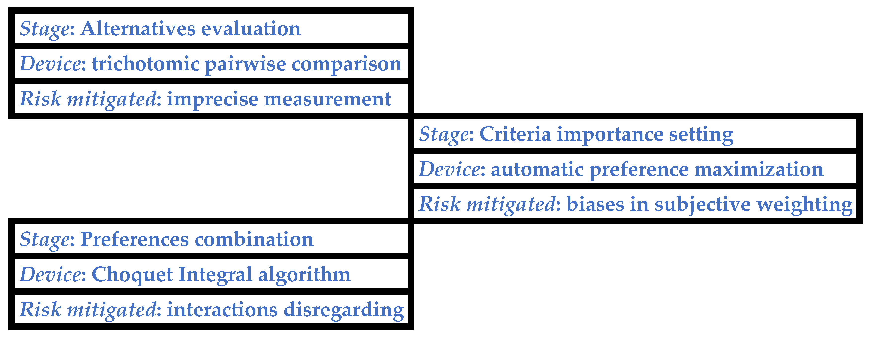
Finally, and more importantly in the search for standards, extracting information on preferences for criteria from available information about preferences for alternatives according to those criteria is simpler and more reliable than asking directly for information about the relative importance of the criteria in abstract comparisons.

Figure 1 highlights the benefits of the introduction in MCDA of the approaches advocated here.

3. Results

This section presents a set of procedures that constitute standards for (i) calculating the preference probabilities according to each criterion, (ii) deriving the capacities of the sets of criteria, and (iii) ranking the alternatives by the Choquet Integral.

3.1. Standards for the Individual Assessments

The probability of preference for each alternative according to each criterion is obtained from evaluations by a sample of the population whose preference is to be measured. Preference probabilities are derived from the values of the trichotomic pairwise comparisons that they produce.

The preference counts are transformed into probabilities by dividing the counts by the total number of evaluations. Let us denote by $C_{ij}$ the count of preferences for the i-th alternative according to the j-th criterion and by $A\left(k,j,i,u\right)$ the result of the trichotomic comparison between alternatives i and u according to the j-th criterion by the k-th evaluator. This result has three possible values: 1 if the k-th evaluator declares i preferable to u, 0 if the evaluator declares u preferable to i, and ½ if the evaluator declares indifference between i and u.

The preference count for i according to the j-th criterion, $C_{ij}$, is the sum

$$C_{ij}={{\displaystyle \sum }}_{ku}A\left(k,j,i,u\right)$$

(1)

for k varying across all the raters evaluating according to criterion j and u ranging over all the alternatives that i is compared with.

This count is, therefore, the sum of the number of pairwise comparisons where i is preferred with half the number of comparisons where i is considered equivalent to another alternative. The estimate of the probability of preference for i is the quotient

$$P_{ij}=C_{ij}/C_j$$

(2)

of the count $C_{ij}$ by the number of comparisons

$$C_j=K_j·N·\left(N-1\right)/2,$$

(3)

for $K_j$, denoting the number of evaluators by the j-th criterion, and N, the total number of alternatives.

The sum of these probabilities is exactly 1.

It is interesting to note that

$$A\left(k,j,i,u\right)=1-A\left(k,j,u,i\right),$$

(4)

granting antisymmetry.

However, the trichotomic pairwise comparison approach avoids the requirement for transitivity [27]. Transitivity need not hold, generally, in the evaluation of preferences. Consider, for instance, the case of ranking a group of tennis players when a criterion may be based on the observation of matches in some number of tournaments. In pairwise comparisons, the evaluator declares a player better than another by looking at the result of a match. It is possible to observe player $i_1$ beating player $i_2$, who beats player $i_3$, while player $i_3$ beats player $i_1$.

3.2. Standards for the Initial Joint Assessments

Once the preference probabilities according to each criterion have been obtained, the criteria capacities that will be used to combine these preference probabilities according to the individual criteria into a global score can be calculated.

Leaving aside the weighting of the criteria and the interactions between them, global scores can be obtained by using the preference counts to directly estimate the preference probabilities for each alternative. Extending the case of only one criterion, in the case of a set J of two or more criteria, a preference score P_iJ for alternative i according to J will then be obtained by adding the $C_{ij}$ given by Equation (1) along the criteria j in J. To avoid implicitly overvaluing those criteria j with a large $K_j$, it will instead be employed thusly:

$$P_{iJ}={{\displaystyle \sum }}_{j\in J}{P}_{ij}.$$

(5)

This initial assessment assumes additivity. Other forms of additive composition are described in [28]. They include probabilistic rules to obtain the preference according to at least one of the criteria in J. Assuming, respectively, the maximum dependence and independence between the indicators involved, $P_{iJ}$ will be given by max _j∈J $P_{ij}$ or by 1 − Π_j∈J(1 − $P_{ij}$). Nevertheless, counting is the easier form of evaluating the effect of joining the criteria.

These counts give all the criteria and all the experts equal importance, although weights can be included if there is sufficient information to consider the ratings differently by distinct criteria or by distinct experts. For instance, to control the effect of any factor unduly raising the preference according to some criteria, when translating the counting $C_{ij}$ into the probabilities of preference $P_{ij}$, the importance of any criterion j may be corrected by applying a proportional reduction to the vector of probabilities of preference according to j (for instance, dividing all $P_{ij}$ by $K_j$_j).

3.3. Standards for Considering Interactions

A capacity on S is a nondecreasing function μ defined on the power set of S with values of 0 at ø and 1 at S. Capacities are not-necessarily additive measures that express, for each subset of S, the subjective importance associated with that subset.

Estimates of the capacities of the criteria can be obtained directly from the experts’ evaluations. However, it is simpler to extract them from the preference counts.

Starting with the preferences according to each subset of criteria above denoted $P_{iJ}$, the principle of concentration of preferences leads to the measurement of the capacities as proportional to the vector of maxima along these preferences. The exact capacity values will be obtained by scaling such that a capacity of 1 is assigned to the set of all the criteria.

Formally, the capacity assignment algorithm for the subset J will have the central step of computing, along all the alternatives, the maximum of the joint preference probabilities

$$M\left(J\right)=ma{x}_i{P}_{iJ}.$$

(6)

The final value of the capacity is achieved with the final standardization that consists of dividing by the largest value. Thus, the capacity of J is

$$\mu \left(J\right)=M\left(J\right)/M\left(\mathrm{S}\right).$$

(7)

3.3.1. Simplified Capacities

In the case of a large number of criteria, the above derivation of capacities may be limited to sets with a small number L of criteria, while capacity 1 is assigned to all the sets of a larger size. That, is, while the sets of more than L criteria receive capacity 1, the sets J of 1, 2, … L criteria have the capacity given by

$$\mu \left(J\right)=M\left(J\right)/maxM\left(H\right)$$

(8)

for H varying along the sets of criteria of cardinality L.

This simplification may reduce the importance of the final score of criteria with strong interactions with large sets of criteria. To prevent distortions, computation for a few other small values of L is advisable if the scores for L = 2 do not present a clear preference for a best alternative.

3.3.2. Combination via the Choquet Integral

To consider in the global scores, in addition to the preferences between the criteria, the interactions between them, the preference probabilities according to the isolated criteria are combined via the Choquet Integral.

The Choquet Integral is a form of aggregation used in place of the weighted average when it is possible that interactions between criteria may invalidate the use of compensatory addition.

For any function x = (x₁, ..., x_t), of domain S = {1, ... , t} and values in R⁺, the Choquet Integral of x with respect to the capacity μ on S associates with x the non-negative real number

$$C_{\mu }\left(x\right)={{\displaystyle \sum }}_{j\in S}\left(x_{\tau \left(j\right)}-x_{\tau \left(j-1\right)}\right)·\mu \{\tau \left(j\right), ... , \tau \left(t\right)\},$$

(9)

for τ denoting a permutation of S such that

x_τ(1) ≤ x_τ(2) ≤ ... ≤ x_τ(t−1) ≤ x_τ(t) and x_τ(0) = 0.

(10)

The Choquet Integral is equivalently given replacing (9) by

$$C_{\mu }\left(x\right)={{\displaystyle \sum }}_{j\in S}{x}_{\tau \left(j\right)}·[\mu (Z_{\tau \left(j\right)})-\mu (Z_{\tau \left(j+1\right)})]$$

(11)

for

$$Z_{\tau \left(j\right)}=\left\{\mathsf{\tau }\right(j), ... , \mathsf{\tau }(t\left)\right\},$$

(12)

for all j from 1 to t, and

$$Z_{\tau \left(t+1\right)}=ø.$$

(13)

When combining preferences via the Choquet Integral, one is also following the principle of concentration of preferences. In fact, the Choquet Integral assigns greater value to the highest preferences if they are obtained by applying a criterion with greater positive interactions with other criteria and lesser value otherwise.

To see how this happens, let us consider the case of only two criteria. If the interaction between the two is positive, the capacity (equal to 1) of the set of both criteria is greater than the sum of the capacities of each in isolation. Thus, the integral value is closer to the highest value than the arithmetic mean is. In fact, the integral is the sum of the smallest value and the product of the multiplication of the difference between the two values by the complement of that smallest capacity, and this complement is higher than the capacity of the second criterion if there is positive interaction and lower if there is negative interaction. In the weighted average, this complement would be replaced by the capacity of the second criterion.

4. Discussion

A discussion of the results is developed here based on the application of the proposed standards to two numerical examples.

4.1. First Example

Let us first consider a case of 100 alternatives evaluated based on four criteria. For illustrative purposes, this case may be thought of as a choice among 100 candidates for some position in a representative democracy. They are evaluated according to four criteria, which may be related to their commitment to objectives concerning fiscal balance, inducement of economic development, social action, and environmental protection, for instance.

Table 1. Counts of preference by criterion.

Alternative	C11	C12	C13	C21	C22	C23	C31	C41
A1	97.5	96.5	97	94	93.5	96.5	99	96
A2	97.5	96.5	97	94	98	96.5	96	97
A3	97.5	93	97	98	95.5	96.5	98	94
A4	97.5	96.5	97	96	98	96.5	94	95
A5	94	96.5	93	94	93.5	93	95	98
A6	94	96.5	97	98	98	96.5	93	93
A7	94	96.5	94	98	95.5	96.5	97	99
A8	92	91.5	91	91.5	91.5	91	90.5	91.5
A9	91	91.5	91	91.5	91.5	91	90.5	90
A10	90	90	91	90	90	91	92	91.5
A1	89	89	89	89	89	89	89	89
A12/A100	44	44	44	44	44	44	44	44

presents the preference counts resulting from the trichotomic pairwise comparison of the alternatives. The first 11 numerical rows present the counts for the first 11 alternatives, A1 to A11. The other alternatives, of smaller preference, have all the same counts shown in the last row. For the first two criteria, C1 and C2, the evaluations are obtained from three experts, C11, C12, and C13 for the first criterion and C21, C22, and C23 for the second criterion. The last two columns present unique counts C31 and C41 for the last two criteria, C3 and C4, possibly derived from comparisons of party platforms. The score 89 for A11 according to each criterion may be associated to this alternative being always evaluated as worse than the first 10 and better than the last 89, and the score 44 for the last 89 alternatives, from A12 to A100, may be associated to them being tied and evaluated as worse than the other 11.

By dividing the count values by the total number of comparisons for each alternative, of 4950 for the last two criteria and three times that number for the first two criteria, the probabilities of preference for each alternative according to each criterion are obtained. Their values are shown in

Table 2. Probabilities of preference by criterion.

Alternative	C1	C2	C3	C4
A1	0.019596	0.019125	0.020000	0.019394
A2	0.019596	0.019428	0.019394	0.019596
A3	0.019360	0.019529	0.019798	0.018990
A4	0.019596	0.019562	0.018990	0.019192
A5	0.019091	0.018889	0.019192	0.019798
A6	0.019360	0.019697	0.018788	0.018788
A7	0.019158	0.019529	0.019596	0.020000
A8	0.018485	0.018451	0.018283	0.018485
A9	0.018418	0.018451	0.018283	0.018182
A10	0.018249	0.018249	0.018586	0.018485
A11	0.017980	0.017980	0.017980	0.017980
A12 a A100	0.008889	0.008889	0.008889	0.008889

. For each column of probabilities, the sum of the values of the first 11 rows with 89 times the value of the last row is equal to 1.

In

Table 3. Capacities of the criteria by ceiling.

Criteria	L = 2	L = 3	Full
{C1}	0.494898	0.331435	0.250323
{C2}	0.497449	0.333144	0.251613
{C3}	0.505102	0.338269	0.255484
{C4}	0.505102	0.338269	0.255484
{C1,C2}	0.988946	0.662301	0.500215
{C1,C3}	1	0.669704	0.505806
{C1,C4}	0.989796	0.662870	0.500645
{C2,C3}	0.993197	0.665148	0.502366
{C2,C4}	0.998299	0.668565	0.504946
{C3,C4}	1	0.669704	0.505806
{C1,C2,C3}	1	0.993166	0.750108
{C1,C2,C4}	1	0.992597	0.749677
{C1,C3,C4}	1	0.997722	0.753548
{C2,C3,C4}	1	1	0.755269

, it can be seen how the capacities change with the ceiling L. In Table 3, omitted is the capacity null for the empty set and 1 for the set of all four criteria.

It can be noted in Table 3 that, among the subsets of two criteria, the one with the highest capacity is formed by C1 and C3, which receives capacity 1 for L = 2. Notwithstanding, C1 is out of the set of three criteria with the highest capacity.

Table 4. Final Scores for 3 capacities.

Alternative	L = 2	L = 3	Full
A1	0.079200	0.078661	0.078132
A2	0.078377	0.078156	0.078014
A3	0.078654	0.078243	0.077684
A4	0.078299	0.077788	0.077340
A5	0.077992	0.077452	0.076988
A6	0.078086	0.077117	0.076636
A7	0.079200	0.078842	0.078301
A8	0.073938	0.073889	0.073704
A9	0.073731	0.073530	0.073334
A10	0.074143	0.073765	0.073577
A11	0.071919	0.071919	0.071919
A12/A100	0.035556	0.035556	0.035556

presents the final scores.

In Table 4, it can be seen how the variation in the capacities affects the final decision. Evident is the highest preference for alternative A7, with a tie with A1 if the simpler capacity resulting from assigning capacity 1 to all the sets of more than two criteria is employed.

4.2. Second Example

As our second example, we consider a real case with a number of criteria that is both larger than usual and larger than the number of alternatives.

It is based on data from [29], of a study of failure mode and effects analysis (FMEA) in the nuclear energy industry. In that study, a hybrid approach to FMEA was designed to handle high-risk environments considering two human reliability dimensions of intelligibility and stress in addition to the classical FMEA dimensions of severity, occurrence, and detectability. This led to the consideration of a set of nine factors: severity of the impact on people (S), on the facilities (F) and on the environment (E), frequency of occurrence (O), undetectability (U), complexity (C), time to diagnosis (T), workload (W), and duration of stressful tasks (D). In [30], ten main modes of human failure following a failure in the external source of energy were identified, which characterized successive stages of risk control. They are summarized in

Table 5. Modes of failure situations.

Mode of Failure	Situation
M1	align replacement generator
M2	manually activate water feed pump
M3	timely activate emptying tank prevention
M4	restore auxiliary feedwater system
M5	start bleed and feed
M6	close motorized isolation valve
M7	close manual valves
M8	establish safety injection
M9	start long-term refrigeration component
M10	align suction from containment well

.

In [29], these modes of failure were evaluated by a team of experts separately considering each of the nine factors. Here, instead, the aim is to employ the values of these evaluations to rank the nine factors. The idea is to obtain information useful for the development of risk management strategies based on the actions taken to control the factors to address the situations represented by the modes of failure.

The first step of this analysis is, then, the counting of pairs of factors with higher evaluation for each factor. The approximate measurements of [29] are presented in

Table 6. Evaluation of 10 modes of failure according to 9 factors.

Mode of Failure	P	F	E	O	D	C	T	W	D
M1	0.09	0.08	0.08	0.20	0.07	0.06	0.05	0.09	0.09
M2	0.03	0.03	0.03	0.10	0.09	0.05	0.04	0.03	0.03
M3	0.27	0.06	0.08	0.08	0.11	0.05	0.05	0.27	0.02
M4	0.06	0.03	0.03	0.13	0.09	0.05	0.04	0.06	0.03
M5	0.12	0.23	0.16	0.08	0.09	0.08	0.05	0.12	0.09
M6	0.06	0.04	0.04	0.06	0.14	0.19	0.28	0.06	0.26
M7	0.12	0.08	0.08	0.08	0.11	0.25	0.23	0.12	0.21
M8	0.07	0.12	0.19	0.10	0.11	0.16	0.15	0.07	0.21
M9	0.06	0.15	0.16	0.06	0.09	0.05	0.08	0.06	0.02
M10	0.12	0.19	0.16	0.08	0.11	0.06	0.06	0.12	0.04

, and the results of the trichotomic counts for each factor according to each mode of failure, divided by the total of 36 comparisons, are presented in

Table 7. Evaluation of the 9 factors according to the 10 modes of failure.

Mode of Failure	P	F	E	O	U	C	T	W	D
M1	0.17	0.10	0.10	0.22	0.06	0.03	0.00	0.17	0.17
M2	0.06	0.06	0.06	0.22	0.19	0.17	0.14	0.06	0.06
M3	0.21	0.08	0.13	0.13	0.17	0.04	0.04	0.21	0.00
M4	0.15	0.03	0.03	0.22	0.19	0.11	0.08	0.15	0.03
M5	0.15	0.22	0.19	0.04	0.10	0.04	0.00	0.15	0.10
M6	0.08	0.01	0.01	0.08	0.14	0.17	0.22	0.08	0.19
M7	0.13	0.03	0.03	0.03	0.08	0.22	0.19	0.13	0.17
M8	0.01	0.11	0.19	0.06	0.08	0.17	0.14	0.01	0.22
M9	0.08	0.19	0.22	0.08	0.17	0.03	0.14	0.08	0.00
M10	0.15	0.22	0.19	0.08	0.11	0.04	0.04	0.15	0.00

. As probabilistic preferences for the modes of failures according to the factors, the values in each column of Table 6 sum 1. The same is true for Table 7 since there the columns are filled by the vectors of measures of preference for the factors, which are then compared with reference to the modes of failure.

It can be seen, comparing Table 6 and Table 7, that, if a factor contributes with a high value in the evaluation of a mode of failure, conversely, the mode of failure presents a high value in the evaluation of the factor, but this is not an absolute rule as the evaluations are, in both cases, relative to the whole set of alternatives. For instance, M9 provides the highest evaluation for E in Table 7, while M8 is the mode of failure with the highest evaluation by E.

The application of the composition by the Choquet Integral with respect to the capacities for the values of L from 2 to 9 and full use of the interaction indirect assessments generates the final scores in

Table 8. Final scores for the 9 factors applying 9 capacities.

Factor	L = 2	L = 3	L = 4	L = 5	L = 6	L = 7	L = 8	L = 9	Full
P	0.01840	0.01736	0.01700	0.01648	0.01582	0.01544	0.01494	0.01422	0.01366
F	0.02222	0.02095	0.01925	0.01793	0.01702	0.01644	0.01561	0.01465	0.01408
E	0.02083	0.02037	0.02021	0.01917	0.01828	0.01763	0.01673	0.01570	0.01508
O	0.02222	0.02222	0.02047	0.01884	0.01785	0.01725	0.01650	0.01564	0.01508
U	0.01944	0.01852	0.01791	0.01716	0.01652	0.01615	0.01568	0.01518	0.01477
C	0.01944	0.01852	0.01762	0.01602	0.01490	0.01435	0.01364	0.01291	0.01247
T	0.02049	0.01829	0.01753	0.01646	0.01524	0.01467	0.01399	0.01305	0.01249
W	0.01840	0.01736	0.01700	0.01648	0.01582	0.01544	0.01494	0.01422	0.01366
D	0.02066	0.01933	0.01839	0.01685	0.01545	0.01441	0.01354	0.01262	0.01208

.

The analysis of Table 8 reveals factors E, related to the severity of the environmental impact, and O, occurrence, tied in the first position. E also ranks first for each of the five highest values of L, whereas O is the first for the other three. These factors are thus identified as the more relevant factors to be considered in the management of risks based on the mitigation of the factors. This is consistent with the classical three-dimensional FMEA analysis, which highlights severity and occurrence.

5. Conclusions

This article brings a new approach to MCDA based on the application of standard rules. A set of standards is proposed. Its validity is checked and its usefulness for practical situations of large numbers of alternatives and of criteria is demonstrated.

The combination of preferences based on multiple criteria can be achieved via the simple procedures developed here, which serve as standards for the analysis of complex decisions with a high degree of subjectivity. The simplest standards comprise the combination via the Choquet Integral, the consideration of the interactions between the criteria by assigning importance to the sets of criteria proportional to the highest preference that they assign, and the employment of trichotomic pairwise comparisons in the data collection.

The strategy for criteria evaluation proposed is designed to concentrate preferences. It is based on the information on preferences for the alternatives according to the criteria instead of on the direct comparison of the criteria.

The results of the application of these standards may serve as a basis for comparison with the application of any MCDA method recommended by the peculiarities of each case. Variations in the capacities, which may amplify the basis of comparison, were studied in practical applications, presenting consistent results.