Mathematical Standard-Parameters Dual Optimization for Metal Hip Arthroplasty Wear Modelling with Medical Physics Applications

Abstract

Total hip metal arthroplasty (THA) constitutes an important proportion of the standard clinical hip implant usage in Medical Physics and Biomedical Engineering. A computational nonlinear optimization is performed with two commonly metal materials in Metal-on-Metal (MoM) THA. Namely, Cast Co-Cr Alloy and Titanium. The principal result is the numerical determination of the K adimensional-constant parameter of the model. Results from a new more powerful algorithm than previous contributions, show significant improvements. Numerical standard figures for dual optimization give acceptable model-parameter values with low residuals. These results are demonstrated with 2D and 3D Graphical/Interior Optimization also. According to the findings/calculations, the standard optimized metal-model parameters are mathematically proven and verified. Mathematical consequences are obtained for model improvements and in vitro simulation methodology. The wear magnitude for in vitro determinations with these model parameter data constitute the innovation of the method. In consequence, the erosion prediction for laboratory experimental testing in THA adds valuable information to the literature. Applications lead to medical physics improvements for material/metal-THA designs.

1. Introduction

In general, there are currently three material groups widely used in total hip metal arthroplasty (THA). Namely, ceramic, metal, and polyethylene. The principal components of a THA are cup and head. Clinically, head-cup combinations could be even (CoC, MoM) or uneven (PoM, CoM, PoC). When a polyethylene cup constitutes at least one component of the THA, the bearing is considered soft [1,2,3,4], otherwise the bearing is hard. The wear of the THA implant occurs in-between the head and cup, specifically in erosion and abrasion biotribological phenomena. This biotribological wear-interface is based on complex biomechanical forces distribution and was presented in previous publications [1,2].

Biomaterials in orthopaedics have evolved significantly along several generations [4,5,6,7,8]. Ceramic materials is the generic group whose hardness magnitude is highest. It is followed in order of magnitude by the metal group and then the polyethylene one. In THA research, the wear/changes during post-operational and implant lifetime in patient can be clinically measured in vivo by using a number of imaging techniques available [3,9]. These are usually conventional XR, RSA (radiostereometric analysis), CT (computerized tomography), MRI (magnetic resonance imaging), and variants/combinations of these. Computational geometry, based on imaging systems, can obtain THA post-surgical and long-term evolution, checking the implant fit with radiomarkers. There are geometrical methods based on radiomarkers positioning to get precise evaluations of the implant up-to-date condition(s). For instance, radiomarkers for pre- and post-surgical positioning determination of lumbar artificial disks were clinically/industrially developed [2].

For in vitro THA wear simulations, the methods conjoin experimental work with modelling optimization. The correlation between in vitro and in vivo data-matching is rather difficult. Since the biomechanical loads are combined with almost continuous/variant daily moving and personal dynamics habits at any physical activity, the THA erosion wear constitutes a biomedical complicated factor. The approximate magnitude of its wear along usage-time has to be determined when manufacturing/designing any THA—no matter metal, ceramic, or polyethylene. Metal prostheses/materials are subject, in general, to erosion and corrosion physical of chemical phenomena, and tribocorrosion happens on human plasma medium, when corrosion, due to plasma free radicals, becomes synergic with erosion. Other types of complications are caused by debris particles of the eccentric wear in the acetabular cup or the cup dislocation [10] when bone hardness is weak and screws cannot hold sufficiently. The in vitro experiment of THA devices to obtain tentative/precise erosive data is an important stage in the manufacturing process. However, and additionally, the in vivo measurements differ from the lab experiments. If the THA prostheses fail, post-operative complications could be a serious surgical problem.

Therefore, the use of mathematical models represents a useful/efficacious tool for these predictions. The continuous improvements in modelling, both analytical and in finite elements, is performed with the combination of computational bioengineering meshed with experimental data. In previous contributions [1,2], a number of optimization models were developed with computational-mathematical methods. In consequence, the principal objective of this study was to obtain advances in an analytical model. This result is the numerical determination of the K adimensional-constant parameter of the model.

Formerly [1], a classification of clinical factors related to THA surgery were presented. Namely, the PF-TCF Hip Arthroplasty Functional Treatment Classification [1]. PF are factors depending on the patient, and TCF are technical-clinical factors of the hospital and/or traumatology-orthopedics service.

In summary, this study presents and demonstrates a mathematical optimization method(s) for in vitro wear prediction in dual metal THA, titanium, and cast Co-Cr alloy. A 3D algorithm is developed and then fitted to experimental data. Computational software method(s) are explained and proven. Applications on Medical Physics and Biomedical engineering emerge from the mathematical results.

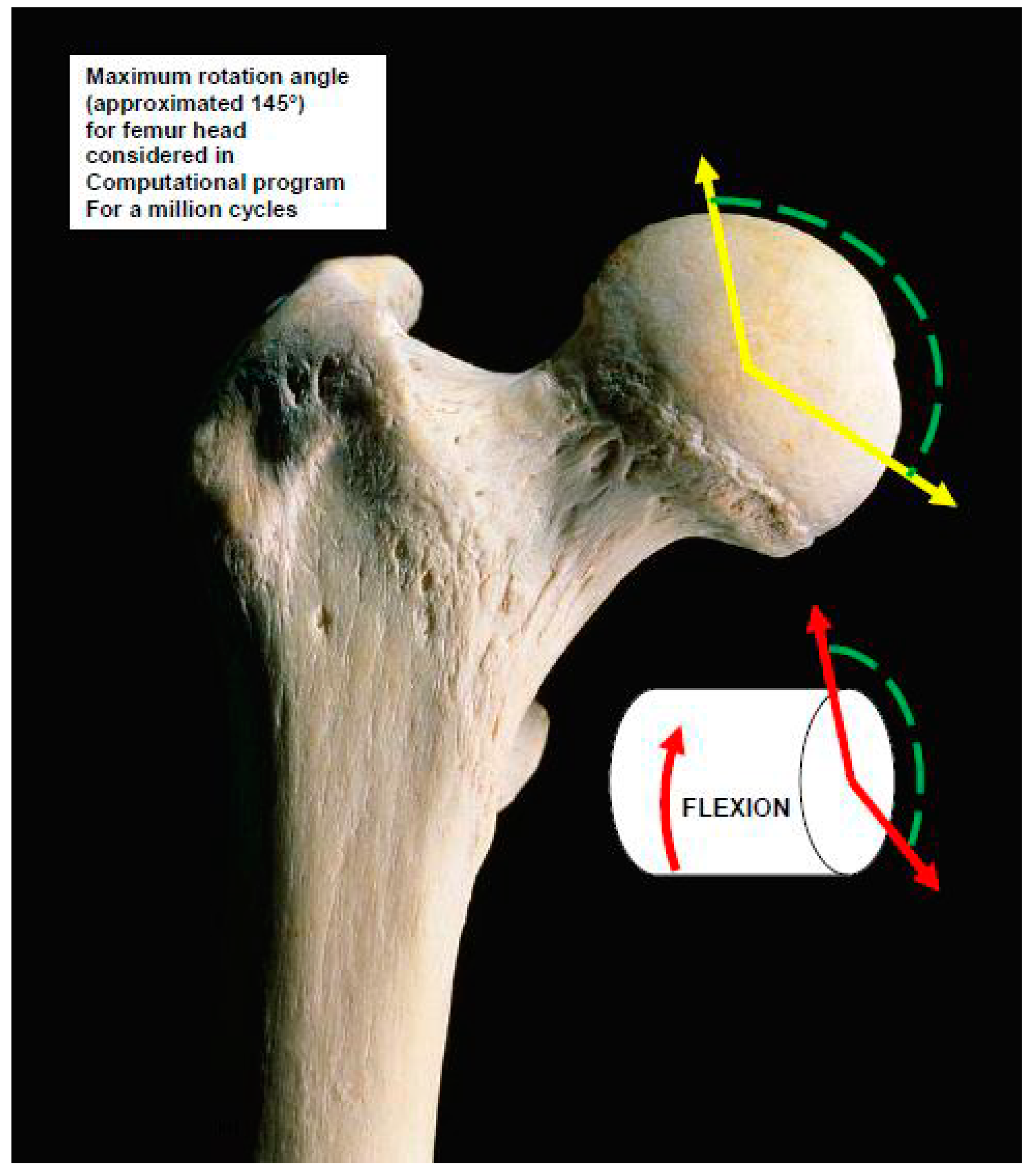
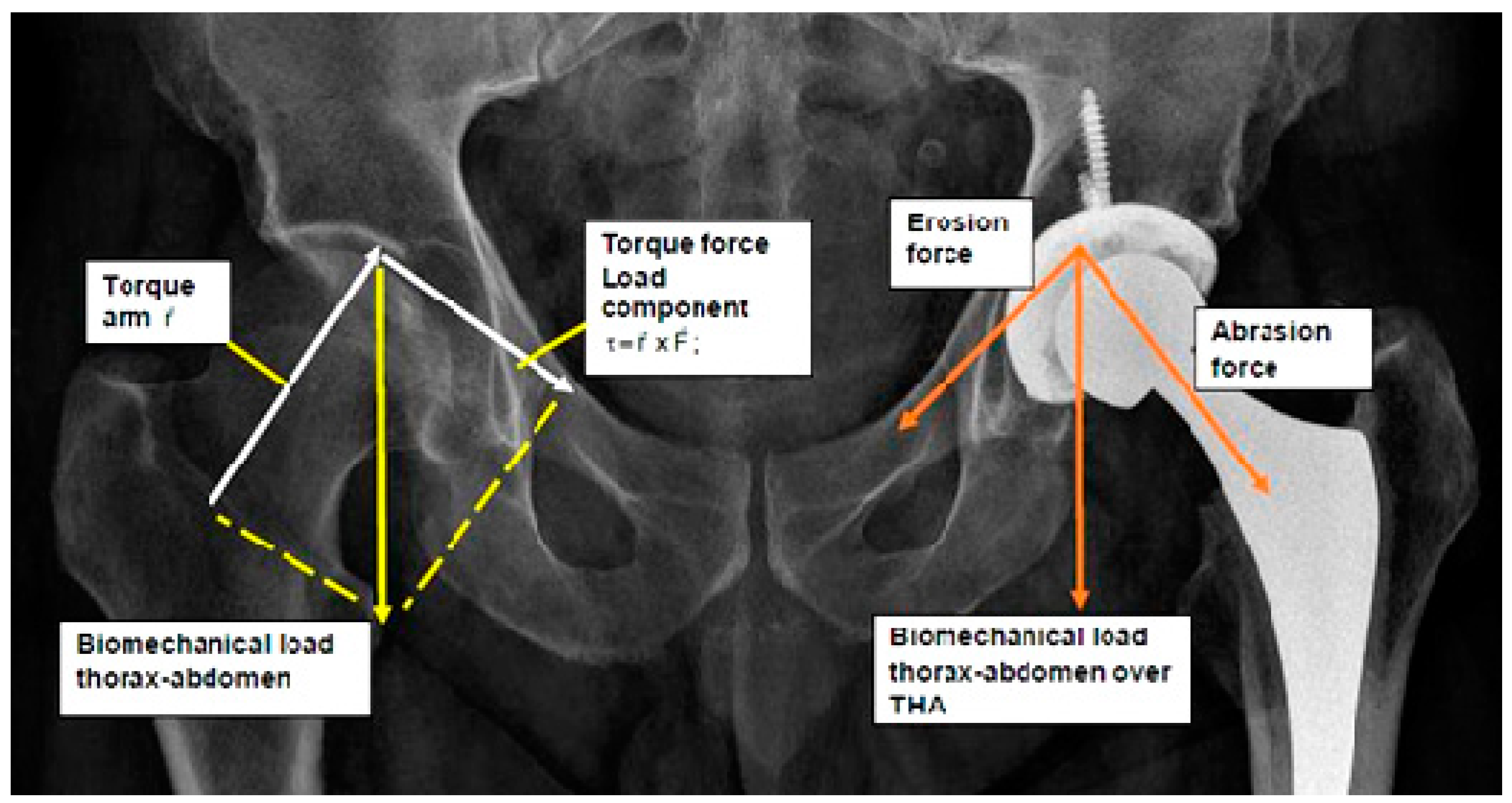
Theoretical and Clinical Biomechanics THA Modelling Pathogenesis with Physics Fundamentals

The pathogenesis of hip articulation malfunction is caused statistically mostly by the high incidence/prevalence of femur neck fracture due to osteoporosis. This happens usually in elderly patients. This incidence/prevalence increases in developed countries in correlation with the increment of the average population age and lifetime expectancy. According to statistics in the European Union and Europe, Germany and Switzerland are the countries where a higher number of THA are surgically implanted/fixed [11,12].

Given a femur neck with osteoporosis [11], as shown in Figure 1, the fracture happens because the head and trochanter are united by the neck, which is the weakest and thinnest bone zone. In addition, the hip load over the femur head causes a mechanical torque whose arm is along the neck and fixed on the trochanter. In other words, the extremes of this physical arm are the femur head and the trochanter. The hip biomechanical-load that makes the torque-magnitude is exerted over the head. Therefore, summing up all these causes, the pathological and biomechanical conditions become synergic in an elderly patient with osteoporosis, whose ligaments and muscles are also weak. When the patient moves abruptly or falls for any reason, the fracture could occur.

In these clinical-surgical circumstances, when a THA is implanted, the medical device is subject to a number of biomechanical forces/parameters. These act on the THA material components and cause mainly wear by erosion and abrasion. The mathematical-physical modelling to determine/measure them precisely is essential, both in vitro (at laboratory with a number of apparatus) and/or in vivo (through several imaging with/without computational geometry methods).

Grosso modo, for in vitro, there are two types of methods, analytical and numerical. Analytical models could involve integral-differential calculus [13,14,15,16], and are usually based on these model variants. The numerical group involves finite element techniques, both linear and nonlinear. In these finite element models, the element wear can be formulated using Archard’s variants [15,17]. A classical analytical method is based on modified Archard’s model Equation (1), which is the focus of this study [1,14,15,16].

Analytical models could be linear and nonlinear [1,14,15,16]. The linear models integrate the hardness within the K parameter. In this study, hardness is considered as an important separated parameter for optimization [1,2,14,15,16]. In the literature, some authors begin developing the nonlinear model through integral-differential calculus and perform finite element calculations [15]. Figure 1 shows a sketch of biomechanical theoretical base for the analytic model. The principal cause of wear in THA is abrasive wear type or three body abrasive wear [14,16].

2. Materials and Methods

Materials selected for dual optimization are cast Co-Cr alloy and titanium. There are several generations of titanium varieties [2,7,8]. Modern beta titanium alloys have metastable physical-chemical useful properties for THA. Their physical characteristics are detailed in

Table 1. Computational implementation numerical data and intervals for optimization.

Programming Numerical Data
Material	Hardness (Hv) and Histocompatibility	Head Diameter (mm)
Cast Co-Cr alloy	300 Average/good	28 [22, 28]
Titanium alloy	362 (approx) /excellent	28 [22, 28]
Optimization Data Intervals
Hardness (GPa)	[2.7, 4.0]
Experimental Erosion (mm3/Mc)	[0.01, 1.8]
Complementary Data	ElasticityModulus and Fracture Thoughness are useful for other type of calculations. The standard femoral head used diameter is 28mm. Cast Co-Cr alloy hardness varies in literature. There are a large number of Titanium alloys available with closely hardness.

. The material and corresponding experimental in vitro erosion data in this study were taken from the literature [3,9]. However, for THA ceramic modelling optimization in previous studies [1], other authors’ and publications were considered [17,18,19,20]. The in vitro wear rates published in [3] constitute acceptable approximated data for model optimization intervals, although in this study the interval-standards published in [9] were implemented in programming. The criteria for testing measurements/units and experimental apparatus varies in the literature [3,9,17,18,19,20,21]. For instance, in [19], the depth of wear for a unit of sliding distance is selected. Other authors [20] chose the criteria in mm³/year, (volumetric wear), or mm/year (linear wear). This research selection is mainly practical for getting precise optimization. In this line, if experimental wear is measured in mm³, it is straightforward guessed that K in Equation (1) becomes adimensional. In all cases, units are adapted on Section 2.1 criteria. Mathematical method(s) and algorithms are explained in Section 2.2. The software implemented constitutes an improvement stage from a former ceramic and metal THA modelling contribution and related publications whose programming tools are similar [1,2,6,22,23,24,25].

2.1. Material and Computational Data

Table 1 shows the material selection data and computational intervals. Provided the units are set in mm, mm³, kg, and s, the standard K parameter of the model becomes adimensional [1,2]. This constitutes an advantage for simplicity/easy calculations with experimental data in vitro.

The hardness of cast Co-Cr alloy is 300 Hv (approximately 3.00 GPa); it is an average value since there are several types of this material. Titanium materials are also manufactured in a number of variant chemical compositions. The average is 362 Hv (approximately 3.62 GPa). The head diameter of the THA is selected as the most frequent standard of 28 mm. Therefore, to make a suitable range of hardness optimization, these hardness values are slightly extrapolated to enlarge the interval extremes, that is, in GPa [2.7, 4.0]. Experimental values are taken from published data [3], and the same technique as hardness interval construction was performed. That is, [0.01, 1.8] mm³ per Mc. Additional material parameters such as elasticity modulus and fracture toughness are important to characterize the material, but not useful for this type of optimization.

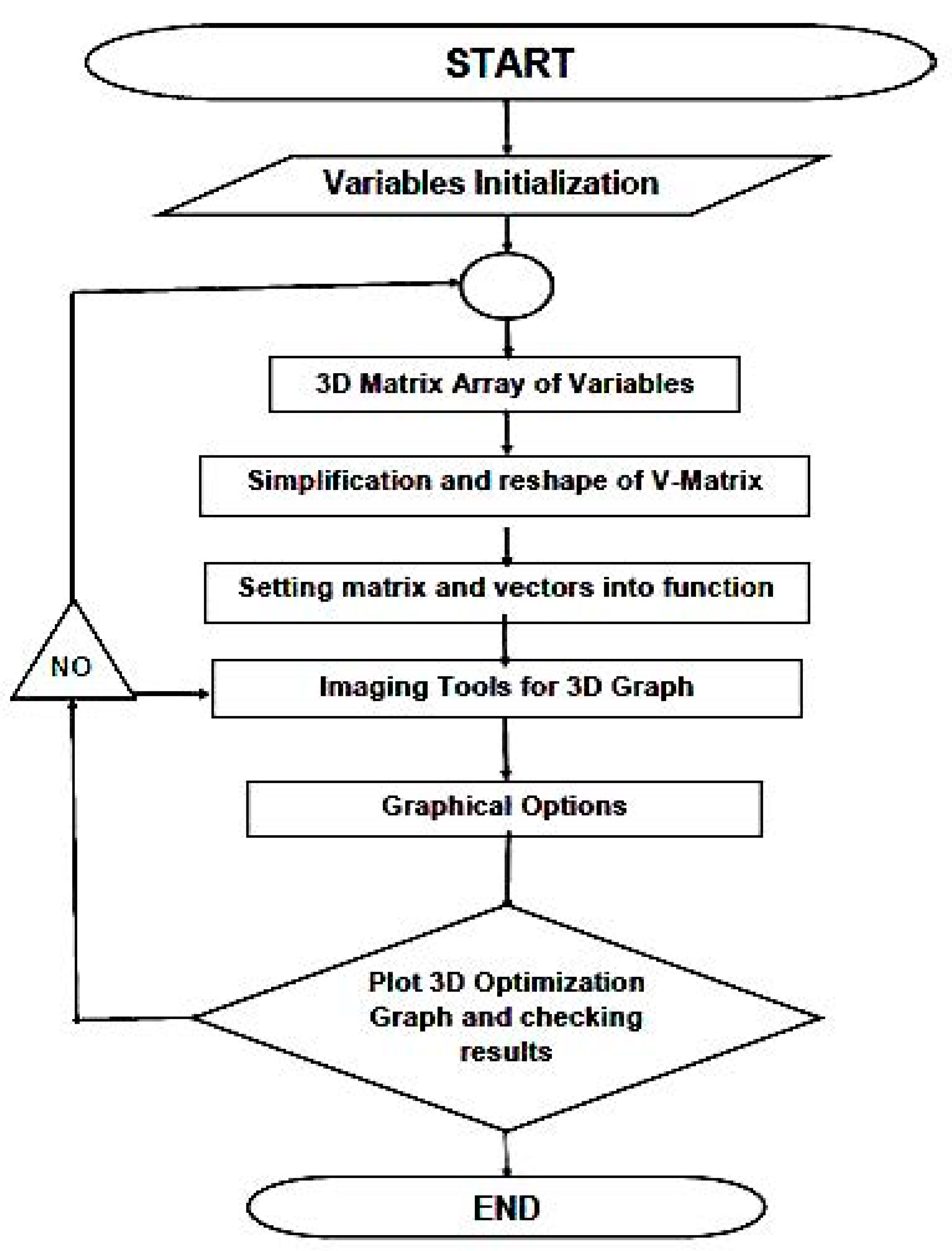
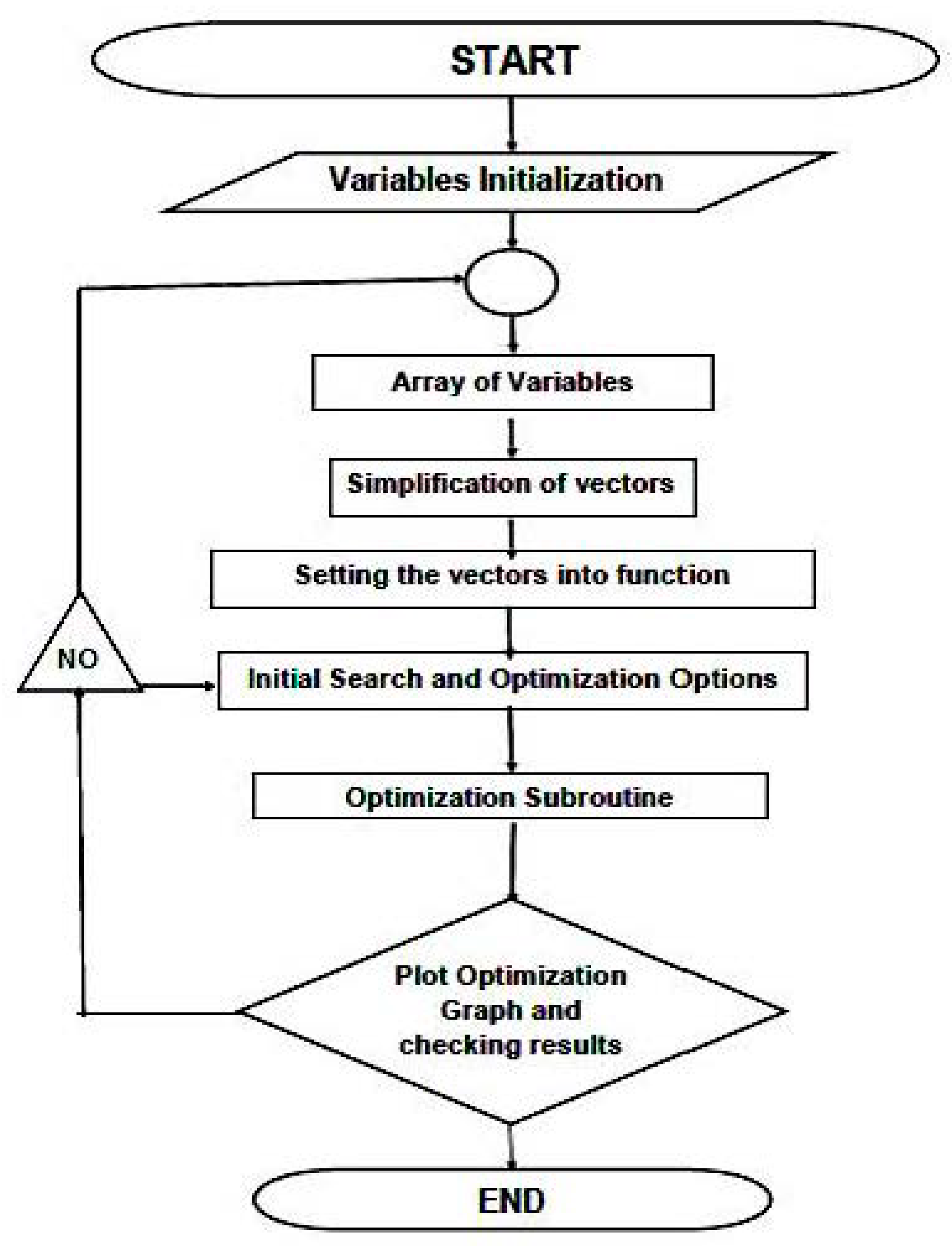
2.2. Optimization Algorithms and Programming-Software Design

The algorithms implemented are based on classical Archard’s model [1,2,14,16], but with vector-matrix and units modifications [1,2]. A variant from this model with evolution algorithms was developed in previous contributions [1,2,24]. The classical equation for wear optimization of hip implants reads,

$$\mathrm{W}\hspace{0.17em}=\hspace{0.17em}\hspace{0.17em}\mathrm{K}\hspace{0.17em}\hspace{0.17em}\frac{\mathrm{L}\times \mathrm{X}}{\mathrm{H}}\hspace{0.17em}\hspace{0.17em}\hspace{0.17em};$$

(1)

where K is the wear constant specific for each material, L is the biomechanical load (N, passed here to kg and mm), X is the sliding distance of the acetabular semi-sphere of the implant (mm), W is the wear (mm³), and H is the hardness of the implant material (MPa, here it is used always as kg and mm). X is measured as the number of rotations of the implant multiplied by half the distance of its circular-spherical length. However, in this study it is better approximated according to human biomechanics and kinesiology. The average rotation of femur head cannot reach 180° at any biomechanical movement in common patients. This is valid for flexion, extension, flexion-rotation, extension-rotation, abduction, adduction, and external/internal rotation [3,19,20]. For the program settings, one cycle is taken as the length corresponding to the maximum kinesiologic rotation angle. The maximum femur rotation angle value is 145° in flexion. In the software, this magnitude is implemented.

A Mc is defined as the length of the femur head circumference during the hip articulation movement (X). That is the standard for many in vitro experimental studies. If at the laboratory the erosion for 1 Mc is determined, then several million cycles (Mcs) can be approximated with the model. Arithmetically, a Mc (a million cycles of femur head during movement) of rotation length is calculated: circumference implant-head radius R by π for a factor of angle of 145° and by 10⁶. Therefore, the erosion in vitro data resulted from this optimization always has to be considered as the maximum possible. Figure 2 shows the biomechanical kinetics for rotation angles implemented in programming. Number of rotations also depends on the daily physical activity of the patient, age, race, genetic heritage, associated diseases, country, sport habits, profession, climate, physical-activity culture, etc.

The load magnitude to be implemented is rather difficult because usually the load is divided in X, Y, Z components [25,26]. Average values and/or forces resultant values are taken. For nonlinear optimization, the average values will be implemented in the program [1,2,26]. In this study, a load of around 200% of body weight (200%BW) is applied for optimization constraints, according to the most usual values of literature [2,3,19,20,26,27]. Constraints for load are set from a 50 kg patient to a 80 kg patient. Fifty kilograms corresponds, for example, to the body weight of elderly women, who present a high incidence/prevalence of femur head fractures.

Model (1) is also used in integral form for finite elements techniques in hip implants. K is a parameter, although in previous contributions, [1,2] this algorithm was implemented for more parameters, such as optimal hardness or number of rotations.

The algorithm is based on vectorial and matrix calculus. These vectors and matrices are set into the software. The parameters such as hardness, load, and experimental wear are set as vectors of 10³ elements within the data interval set. The mathematical operations of these vectors when setting into the model require a careful and precise method to obtain the objective function ready for the subroutine. Least squares optimization method was widely applied in previous studies [2,18,22,24,26,27,28,29,30,31,32,33,34].

Least squares method with L₂ norm is widely used and has the advantage that the OF is always positive. For setting the inverse optimization problem, this technique can be considered acceptable [30,31,32,33].

Therefore, the least squares OF with L₂ norm that is used, [1], without fixed constraints reads,

Minimize,

$${\Vert \overrightarrow{\mathrm{W}}-\overrightarrow{\mathrm{K}}\hspace{0.17em}\frac{\overrightarrow{\mathrm{L}}\times \overrightarrow{\mathrm{X}}}{\overrightarrow{\mathrm{H}}}\Vert }_2^2\hspace{0.17em}\cong \hspace{0.17em}0\hspace{0.17em};\hspace{0.17em}$$

subject to (generically),

$$\left[\begin{array}{c}\mathrm{a}\\ \mathrm{b}\\ \mathrm{c}\\ \mathrm{d}\\ \mathrm{e}\end{array}\right]\hspace{0.17em}\le \hspace{0.17em}\left[\begin{array}{c}\left|{\mathrm{K}}_{\mathrm{i}}\right|\\ \left|{\mathrm{L}}_{\mathrm{i}}\right|\\ \left|{\mathrm{X}}_{\mathrm{i}}\right|\\ \left|{\mathrm{H}}_{\mathrm{i}}\right|\\ \left|{\mathrm{W}}_{\mathrm{i}}\right|\end{array}\right]\hspace{0.17em}\le \hspace{0.17em}\left[\begin{array}{c}{\mathrm{a}}_1\\ {\mathrm{b}}_1\\ {\mathrm{c}}_1\\ {\mathrm{d}}_1\\ {\mathrm{e}}_1\end{array}\right]\hspace{0.17em};$$

(2)

The software and mathematical methods of this contribution constitute both an improved evolution and completely different programs from previous publications [2,22,25,34,35,36] with Matlab and L₂ norm. 2D, Figure 3 and Figure 4, and 3D graphical subroutines have been used in previous contributions [31,33]. In [37], biomechanical data was used to design software. Fortran 90 [22,32] was used to check/validate the numerical precision of the results. Freemat [18,22,32] was used to verify 3D Interior Optimization, as shown in Figure 5, Figure 6, Figure 7, Figure 8 and Figure 9. The variations/improvements are usage of 2D Graphical Optimization and 3D Interior Optimization methods [2,22,35,36]. The software is different in every case. The least-squares OF inverse algorithm [1,2,22,24,32,34] implemented reads,

$$\begin{array}{l}\mathrm{minimize},\\ {\Vert \hspace{0.17em}\mathrm{F}\left(\overrightarrow{\mathrm{W}},\overrightarrow{\mathrm{K}},\overrightarrow{\mathrm{H}},\overrightarrow{\mathrm{L}},\overrightarrow{\mathrm{X}}\right)\Vert }_2^2\hspace{0.17em}\hspace{0.17em}\cong \hspace{0.17em}\dots \\ \dots \cong \hspace{0.17em}\hspace{0.17em}\hspace{0.17em}{\displaystyle \sum _{\mathrm{i}=1}^{\mathrm{i}=\mathrm{N}}}{\displaystyle \sum _{\mathrm{j}=1}^{\mathrm{j}=\mathrm{N}}}\dots \\ \dots {\displaystyle \sum _{\mathrm{k}=1}^{\mathrm{k}=\mathrm{N}}({\mathrm{F}}_{\mathrm{i}\mathrm{j}\mathrm{k}}{\left({\mathrm{W}}_{\mathrm{i}\mathrm{j}\mathrm{k}},{\mathrm{K}}_{\mathrm{i}\mathrm{j}\mathrm{k}},{\mathrm{H}}_{\mathrm{i}\mathrm{j}\mathrm{k}},{\mathrm{L}}_{\mathrm{i}\mathrm{j}\mathrm{k}},{\mathrm{X}}_{\mathrm{i}\mathrm{j}\mathrm{k}}\right)}^2\hspace{0.17em}+\dots }\\ \dots +{\mathrm{F}}_{\mathrm{N}}{\left({\mathrm{W}}_{\mathrm{N},\mathrm{N},\mathrm{N}},{\mathrm{K}}_{\mathrm{N},\mathrm{N},\mathrm{N}},{\mathrm{H}}_{\mathrm{N},\mathrm{N},\mathrm{N}},{\mathrm{L}}_{\mathrm{N},\mathrm{N},\mathrm{N}},{\mathrm{X}}_{\mathrm{N},\mathrm{N},\mathrm{N}}\right)}^2);\\ \mathrm{s}\mathrm{u}\mathrm{b}\mathrm{j}\mathrm{e}\mathrm{c}\mathrm{t}\hspace{0.17em}\mathrm{g}\mathrm{e}\mathrm{n}\mathrm{e}\mathrm{r}\mathrm{i}\mathrm{c}\mathrm{a}\mathrm{l}\mathrm{l}\mathrm{y}\hspace{0.17em}\mathrm{t}\mathrm{o},\\ \left[\begin{array}{c}\mathrm{a}\\ \mathrm{b}\\ \mathrm{c}\\ \mathrm{d}\\ \mathrm{e}\end{array}\right]\hspace{0.17em}\le \hspace{0.17em}\left[\begin{array}{c}\left|{\mathrm{K}}_{\mathrm{i}}\right|\\ \left|{\mathrm{L}}_{\mathrm{i}}\right|\\ \left|{\mathrm{X}}_{\mathrm{i}}\right|\\ \left|{\mathrm{H}}_{\mathrm{i}}\right|\\ \left|{\mathrm{W}}_{\mathrm{i}}\right|\end{array}\right]\hspace{0.17em}\le \hspace{0.17em}\left[\begin{array}{c}{\mathrm{a}}_1\\ {\mathrm{b}}_1\\ {\mathrm{c}}_1\\ {\mathrm{d}}_1\\ {\mathrm{e}}_1\end{array}\right]\hspace{0.17em};\end{array}$$

(3)

K is the principal variable for optimization. The reason is that with a multiobjective K parameter it is possible to carry out in vitro simulations in the materials selection process. The hardness for simulations in vitro, within the optimization hardness interval, could, therefore, be different than titanium and/or cast Co-Cr alloy [6]. Constraints are selected as follows,

$$\begin{array}{l}\mathrm{minimize}\hspace{0.17em}\mathrm{O}\mathrm{F},\hspace{0.17em}\mathrm{s}\mathrm{u}\mathrm{b}\mathrm{j}\mathrm{e}\mathrm{c}\mathrm{t}\hspace{0.17em}\mathrm{t}\mathrm{o},\\ \mathrm{N}=\hspace{0.17em}2\times {10}^6\hspace{0.17em},\\ \forall \hspace{0.17em}\mathrm{W}\in \overrightarrow{\mathrm{W}}\hspace{0.17em},\hspace{0.17em}\mathrm{H}\in \hspace{0.17em}\hspace{0.17em}\overrightarrow{\mathrm{H}}\hspace{0.17em},\hspace{0.17em}\mathrm{L}\in \hspace{0.17em}\hspace{0.17em}\overrightarrow{\mathrm{L}}\hspace{0.17em},\hspace{0.17em}\mathrm{X}\in \hspace{0.17em}\overrightarrow{\mathrm{X}}\hspace{0.17em},\\ 0.01\hspace{0.17em}\le \hspace{0.17em}\left|\mathrm{W}\right|\hspace{0.17em}\le \hspace{0.17em}1.8\mathrm{m}{\mathrm{m}}^3\hspace{0.17em},\\ 2.7\times {10}^6\hspace{0.17em}\le \hspace{0.17em}\left|\mathrm{H}\right|\hspace{0.17em}\le \hspace{0.17em}4.0\times {10}^6\hspace{0.17em}\mathrm{kg},\mathrm{mm}\hspace{0.17em};\\ 7.5\times {10}^4\times 9.8066\hspace{0.17em}\le \hspace{0.17em}\left|\mathrm{L}\right|\hspace{0.17em}\le \hspace{0.17em}2.0\times {10}^5\times 9.8066\hspace{0.17em}\left(200\%\hspace{0.17em}\mathrm{B}\mathrm{W}\right);\\ \Vert \overrightarrow{\mathrm{X}}\Vert \hspace{0.17em}=\hspace{0.17em}\mathrm{\pi }\times 28\times (145\times {10}^6)/180\hspace{0.17em}(1\hspace{0.17em}\mathrm{Million}\hspace{0.17em}\mathrm{cycles})\hspace{0.17em};\end{array}$$

(4)

Provided this OF and constraints, the running program time resulted in between 2–8 min, with a standard current microprocessor and pc memory. 3D Interior Optimization takes a longer time because the number of nested arrays and patterns is higher than 2D Graphical Optimization. Scale factors are essential in both types of codes for sharp visualization [1,2,22,24,32].

Figure 3 and Figure 4 show flowcharts for 2D Graphical Optimization and 3D Interior Optimization software design. Both programs demand a high level of precision and systematic consistency. The 2D Graphical Optimization program has several variants corresponding to the choice of the selected parameter for optimization, as visualized on the graph.

3. Results

The numerical results are obtained both from the optimization algorithm program numerical output and 2D Graphical and Interior Optimization charts;

Table 2. Summary of numerical results.

Dual 2D Optimization Results and 3D Interior Optimization Results
Material	Optimal K Adimensional	Optimal Hardness (kg, mm)
Cast Co-Cr alloy	28.93 × 10−9 (truncated)	3.05 × 106 (truncated)
Titanium
Residual for Optimal K	660.44 × 103 (truncated)
3D Interior Optimization Results
3D matrix Program	Validation of K optimal adimensional parameter. In chart. Validation of erosion rises when Hardness decreases

shows all the numbers. The first figures that are obtained are the optimal K (local minimum) and the residual. With these values, the search for optimal hardness commences. This numerical tentative exploration is firstly done by using the Graphical Optimization plots—Figure 4 and Figure 5. When plotting hardness interval versus absolute difference between model and experimental results, the concavity shows the optimal harness value with a cursor, as shown in Figure 6.

Once the optimal K and hardness are obtained, the 3D Interior Optimization process starts. Around the K optimal value, a wide interval is set on one axis. The other axis has the dual hardness interval. The Z axis shows the model wear. These 3D plot patterns are designed firstly with a 3D array (10⁵ and 10⁶ element matrices). These 3D volume matrices contain the elements L, H, and K. The plotting result is a 3D Graphical Optimization chart that verifies the optimal K value, since it is around the K optimal value. It is also clear that the erosion is higher at lower values of hardness, and those stair intervals correspond to the increasing loads for every K sub-interval of the array-matrix, as shown in Figure 7, Figure 8 and Figure 9. When doing a 10⁶ array-matrix, the plot results as a solid block that shows the increased erosion when hardness decreases.

3.1. Optimization Numerical Results

The numerical results are presented in Table 2 and can be read from graphics with Matlab. Graphics software was designed to show the local minimum as a function of several parameters. In Table 2, the dual nonlinear optimization for cast Co-Cr alloy and titanium is shown. The optimal K value obtained is 28.9295 × 10⁻⁹ with residual 660.4426 × 10³. The optimal hardness obtained is 3.054 × 10⁶. Figure 4 and Figure 5 show the model 2D Graphical Optimization. The curves and areas correspond to the model objective function (Y axis) related to parameter values (X axis). Nonlinear dual 2D optimization matrix was set with 2 million functions. Running time was about 2–8 min to obtain local minima and graphics. The 2D surfaces obtained are filled with all the OF values for 2 million functions. As it occurred for THA ceramic modelling optimization [1], the exclusive existence of local minima is demonstrated. Residuals are low considering the 2 million OFs of the optimization matrix. 3D Interior Optimization graphs are shown in Figure 6, Figure 7 and Figure 8. These prove the consistency of 2D Graphical and Numerical Optimization. Freemat [22,24] was used to verify 3D graphics and Fortran [5,24] for all numerical results. The Freemat images for 3D Interior Optimization are high quality.

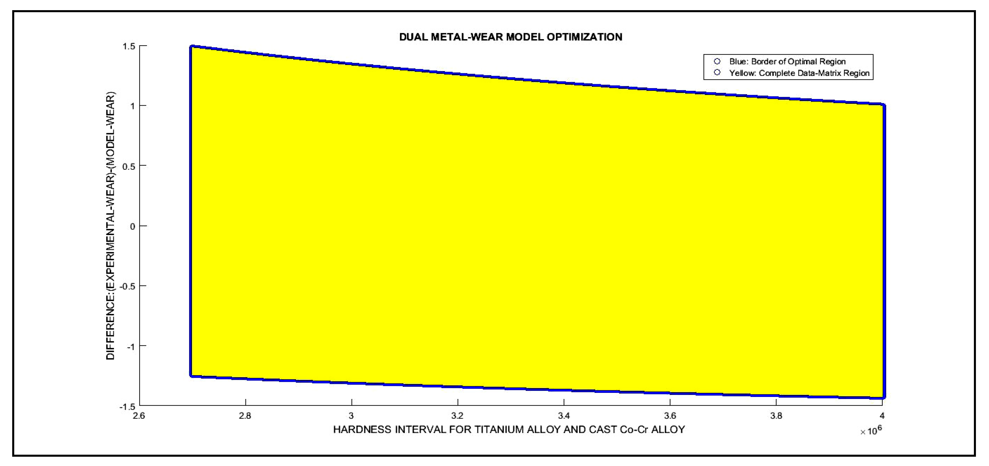
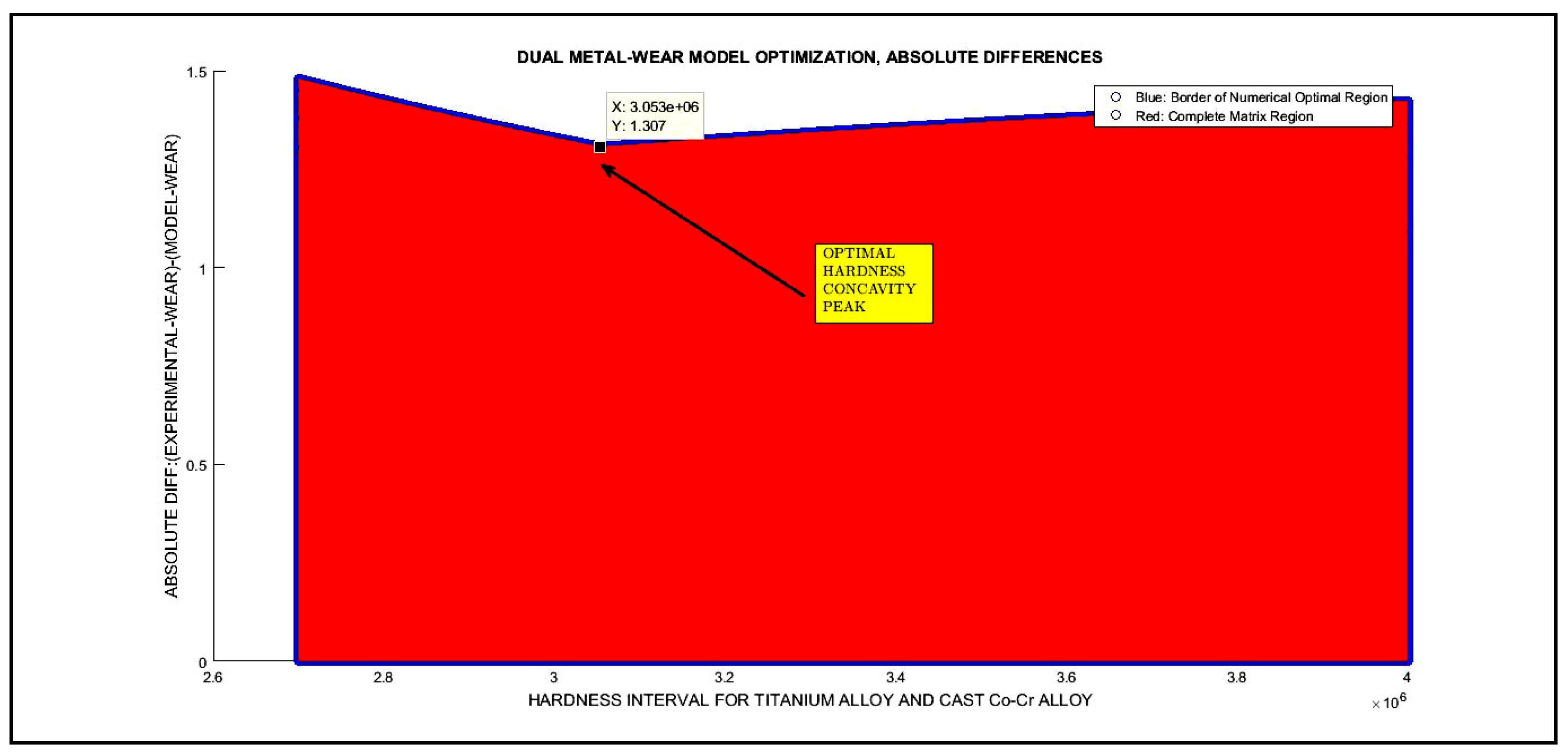
3.2. 2D Optimization Results

The first optimization program has two parts. The first one is related to numerical results for K and optimal hardness. The second is the plotting of 2D Graphical Optimization. Table 1 details numerical results. Figure 5 and Figure 6 show the 2D Graphical Optimization results for about 2 × 10⁶ functions. Figure 5 demonstrates the optimization region and the decrease of erosion when hardness increases and the difference between experimental values and model figures. Figure 6 shows the optimal hardness obtained verification with 2D Graphical Optimization. The optimal K value obtained is 28.9295 × 10⁻⁹ with residual 660.4426 × 10³. The optimal hardness obtained is 3.054 × 10⁶. All numerical values are expressed in mm, mm³, and kg. The K-metal magnitude results are higher than K-ceramic standard parameters for ceramic THA optimization [1,2].

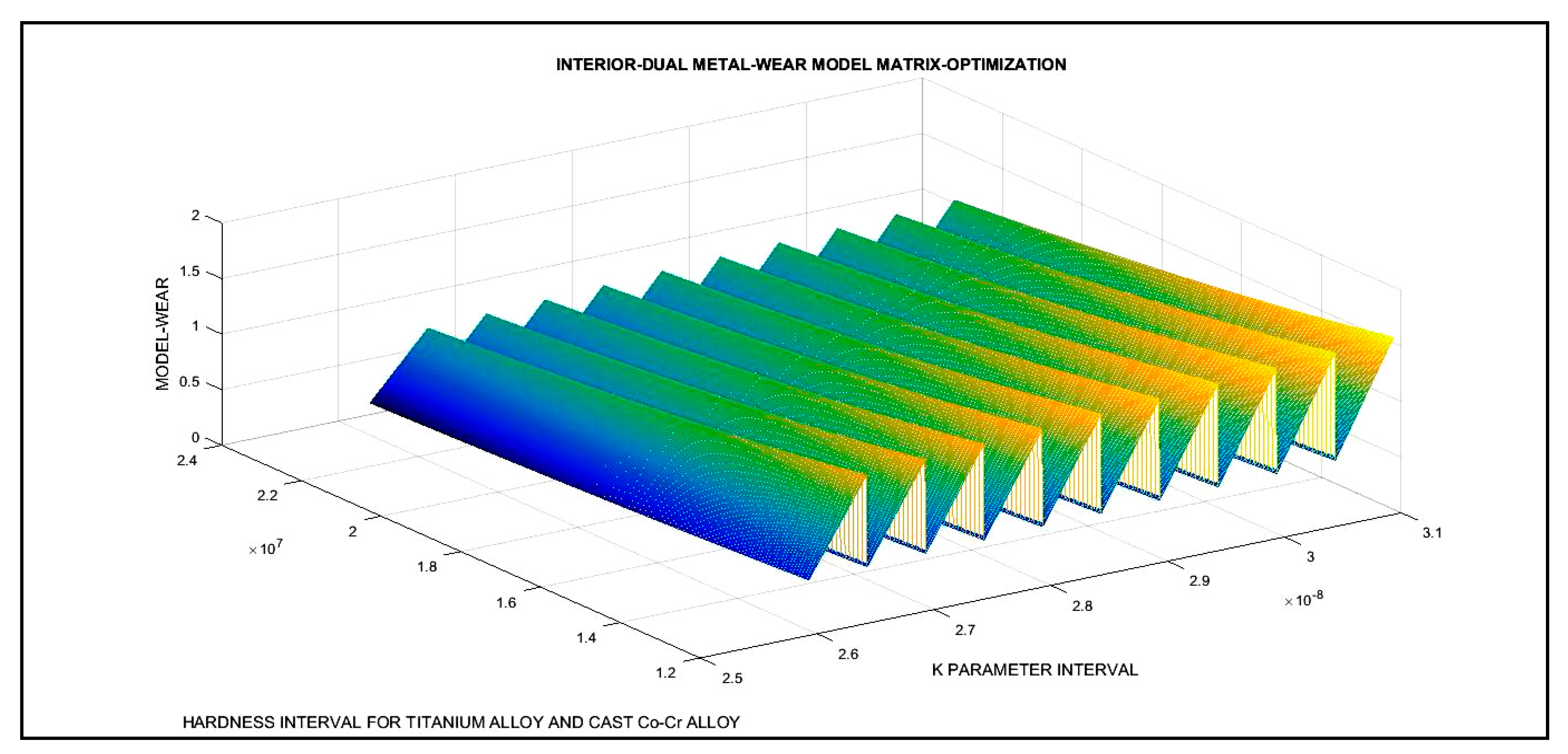
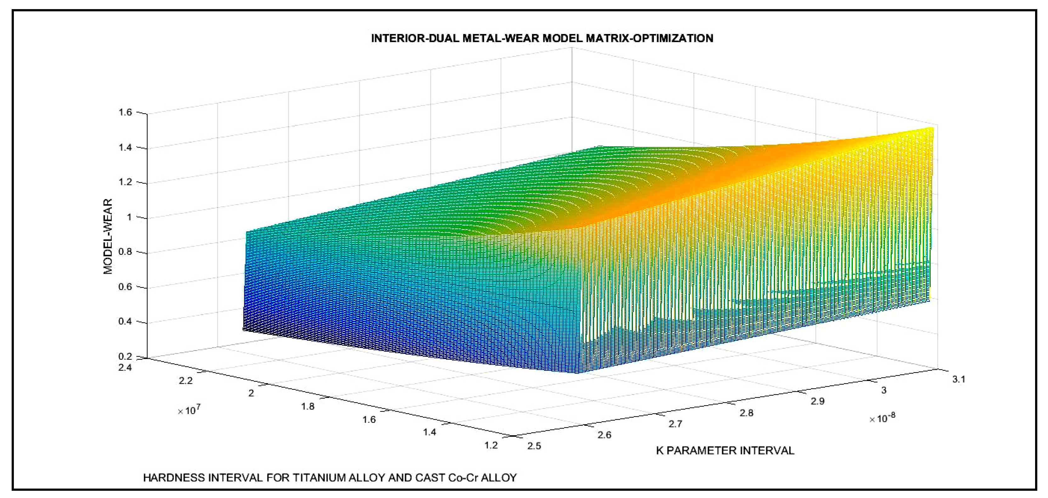
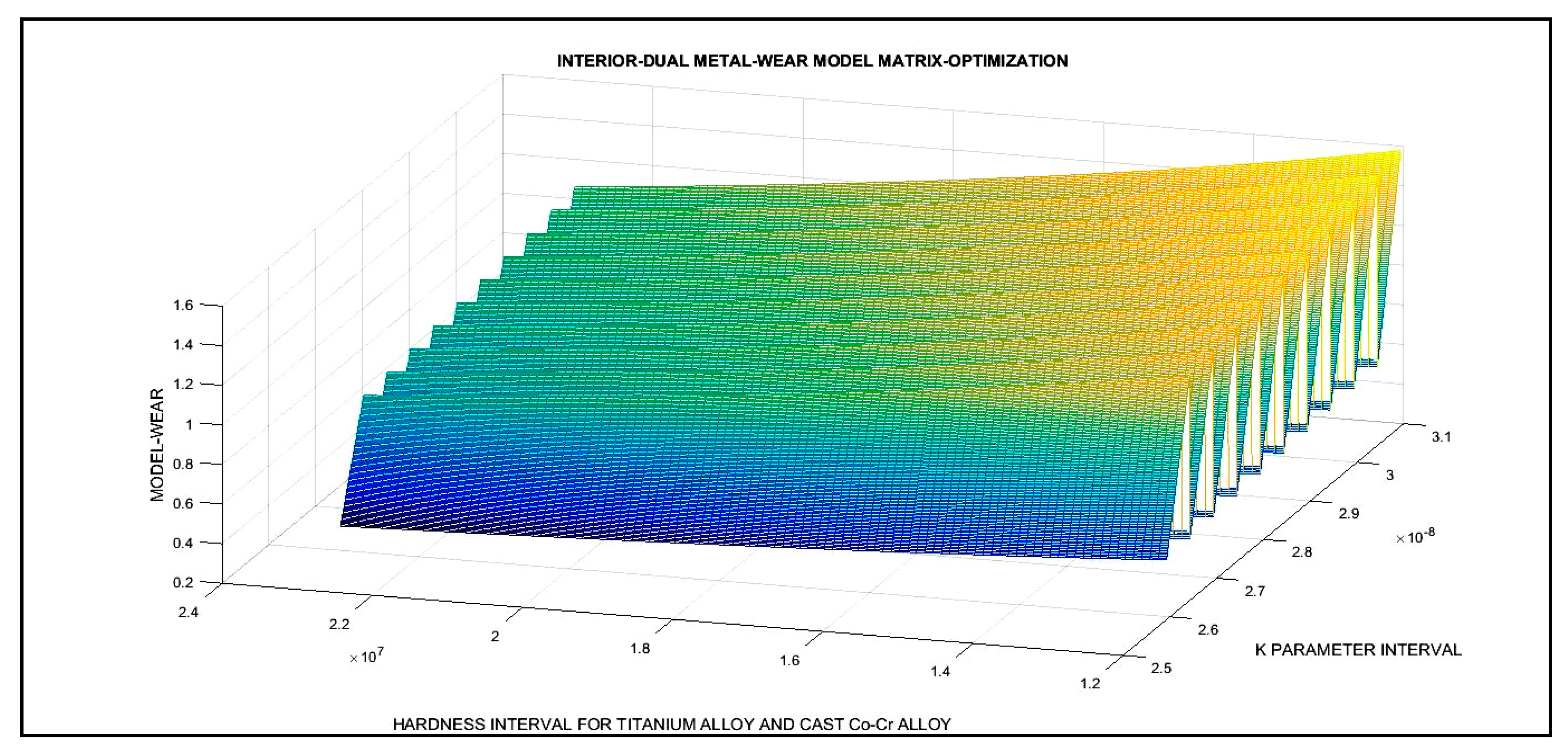
3.3. 3D Optimization Results

Second optimization program(s) are based on nested arrays and a 3D volume-matrix with 10⁵ elements (Figure 7 and Figure 8, first program) and 10⁶ elements (Figure 9, second program). The X axis shows a K interval around the optimal value obtained with the optimization program. The Y axis shows the hardness interval. All numerical values are expressed in mm, mm³, and kg. The software design was rather complicated [1,2,22,24].

3.4. Optimization Numerical Results Verification

The numerical results verification can be checked in two ways. The first one is the 2D and 3D graphics parameters and intervals that provide numerical data distribution. The second is, for instance, to check whether the model optimal values are within the experimental interval. Hence, to verify the numerical results, the optimal values are implemented in the model as follows,

$$\begin{array}{l}\left|\mathrm{K}\left(\mathrm{optimal}\right)\times \frac{\mathrm{Load}\hspace{0.17em}\left(\mathrm{average}\right)\hspace{0.17em}\times \hspace{0.17em}\mathrm{Mc}}{\mathrm{Hardness}\hspace{0.17em}\left(\mathrm{optimal}\right)}\right|\\ =\hspace{0.17em}28.93\times {10}^{-9}\hspace{0.17em}\times \frac{1.10\times {10}^6\times \mathrm{M}\mathrm{c}}{3.05\hspace{0.17em}\times {10}^6}\\ =0.7393\hspace{0.17em}{\mathrm{mm}}^3\hspace{0.17em}\hspace{0.17em}\in \hspace{0.17em}[0.01\hspace{0.17em},\hspace{0.17em}1.8\hspace{0.17em}];\end{array}$$

(5)

This was verified, since 0.7393 mm³ belongs to the experimental interval [0.01, 1.8], approximately at its middle values. This implies that the theoretical model optimization is acceptable and matches the experimental in vitro laboratory measurements.

4. Discussion and Conclusions

An inverse dual optimization study was presented with an improved classical wear model and an original computational algorithm. The model was applied on material wear for metal THA. The selected materials were titanium and cast Co-Cr alloy. The software implemented for the algorithm [1,2] resulted in an acceptable standard K parameter and optimal hardness for the model. It is designed based on previous contributions [38,39,40], and THA/anatomical-physiological contributions [6,41]. The K parameter and optimal hardness can be used for any material wear prediction within the interval model whose parameters were computationally chosen. From a former contribution using this model, the obtained K-metal magnitude is higher compared to K-metal standard parameter [1,2]. Residuals in optimization performance are acceptable. The graphs presented resulted in being sharp with good magnitude visualization. The running time for programs was from 2 to 8 min. 2D Graphical Optimization graphs show the erosion distribution related to hardness. That is useful for wear magnitude prediction when in vitro experiments are carried out. The comparative study with previous research, namely THA erosion wear with the same model, confirms the optimal K figure of this study. The main reason is that the K order of magnitude, in ceramic one order lower, matches the in vitro experimental data with the model. 3D Graphical Optimization gives a range of K values that are also acceptable for wear at the hardness interval with low error dispersion.

The objective of the study was to obtain standard parameters for these two common metal materials in THA. The utility of the results is mainly focused on extrapolated-simulations/predictions of erosion rates for in vitro THA studies. Other variant materials within the selected interval ranges can be implemented in the model whose optimal parameters are determined. Improvements in algorithms, software, and model design are feasible from these findings. The contribution of these results in predictive wear methods is focused on in vitro experimental-computational erosion determinations. This means that the obtained K and hardness values for this model could be used as a numerical exact/approximated reference to get tentative data when planning an experiment. A useful, complementary advantage of the algorithm-model is the setting of K as an adimensional model-constant. That makes the experimental work easier with the units implemented into the model.

In brief, an accurate and efficacious dual optimization to obtain functional modelling parameters in metal THA erosion was presented. Applications in Medical Physics come from all these biotribological modelling improvements.

5. Scientific Ethics Standards

2D/3D Graphical-Optimization Methods were created by Dr Francisco Casesnoves on December 2016, and Interior Optimization Methods in 2019. This software was originally developed by the author. This article uses information from previous papers, whose inclusion is essential to make the contribution understandable. The nonlinear optimization software was improved from previous contributions in subroutines modifications, patterns, loops, graphics, and optimal visualization. This study was carried out according to the European Union Technology and Science Ethics. Reference, ‘European Textbook on Ethics in Research’. European Commission, Directorate-General for Research. Unit L3. Governance and Ethics. European Research Area. Science and Society. EUR 24452 EN [42,43]. And based on The European Code of Conduct for Research Integrity. Revised Edition. ALLEA. 2017.y. Revised Edition. ALLEA. 2017. This research was completely done by the author: The computational-software, calculations, images, mathematical propositions and statements, reference citations, and text are all original from the author. When anything was taken from a source (Figure 1 and Figure 2 free Google Images drawn and modified by Author), it was adequately recognized. Ideas from previous publications were emphasized in the aim of clarification [42,43].

References

1. Casesnoves, F. Multiobjective Optimization for Ceramic Hip Arthroplasty with Medical Physics Applications. Int. J. Sci. Res. Comput. Sci. Eng. Inf. Technol. 2021, 7, 582–598. [Google Scholar] [CrossRef]
2. Casesnoves, F. Nonlinear comparative optimization for biomaterials wear in artificial implants technology. In Proceedings of the Applied Chemistry and Materials Science RTU2018 Conference Proceedings, Riga, Latvia, 26 October 2018. [Google Scholar]
3. Merola, M.; Affatato, S. Materials for Hip Prostheses: A Review of Wear and Loading Considerations. Materials 2019, 12, 495. [Google Scholar] [CrossRef] [Green Version]
4. Navarro, N. Biomaterials in orthopaedics. J. R. Soc. Interface 2008, 5, 1137–1158. [Google Scholar] [CrossRef] [Green Version]
5. Kurtz, S. Advances in Zirconia Toughened Alumina Biomaterials for Total Joint Replacement. J. Mech. Behav. Biomed. Mater. 2014, 31, 107–116. [Google Scholar] [CrossRef] [Green Version]
6. Sachin, G.; Mankar, A.; Bhalerao, Y. Biomaterials in Hip Joint Replacement. Int. J. Mater. Sci. Eng. 2016, 4, 113–125. [Google Scholar] [CrossRef]
7. Li, Y.; Yang, C.; Zhao, H.; Qu, S.; Li, X.; Li, Y. New Developments of Ti-Based Alloys for Biomedical Applications. Materials 2014, 7, 1709–1800. [Google Scholar] [CrossRef] [Green Version]
8. Kolli, R.; Devaraj, A. A Review of Metastable Beta Titanium Alloys. Metals 2018, 8, 506. [Google Scholar] [CrossRef] [Green Version]
9. Holzwarth, U.; Cotogno, G. Total Hip Arthroplasty. JRC Scientific and Policy Reports; European Commission: Brussels, Belgium, 2012. [Google Scholar]
10. Delimar, D. Femoral head wear and metallosis caused by damaged titanium porous coating after primary metal-on-polyethylene total hip arthroplasty: A case report. Croat. Med. J. 2018, 59, 253–257. [Google Scholar] [CrossRef] [PubMed] [Green Version]
11. Zhang, M.; Fan, Y. Computational Biomechanics of the Musculoskeletal System; CRC Press: Boca Raton, FL, USA, 2015. [Google Scholar]
12. Dreinhöfer, K.; Dieppe, P.; Günther, K.; Puhl, W. Eurohip. Health Technology Assessment of Hip Arthroplasty in Europe; Springer: Berlin/Heidelberg, Germany, 2009. [Google Scholar]
13. Casesnoves, F. 2D computational-numerical hardness comparison between Fe-based hardfaces with WC-Co reinforcements for Integral-Differential modelling. Trans. Tech. 2018, 762, 330–338. [Google Scholar] [CrossRef]
14. Hutchings, I.; Shipway, P. Tribology Friction and Wear of Engineering Materials, 2nd ed.; Elsevier: Amsterdam, The Netherlands, 2017. [Google Scholar]
15. Shen, X.; Lei, C.; Li, R. Numerical Simulation of Sliding Wear Based on Archard Model. In Proceedings of the 2010 International Conference on Mechanic Automation and Control Engineering, Wuhan, China, 26–28 June 2010. [Google Scholar] [CrossRef]
16. Affatato, S.; Brando, D. Introduction to Wear Phenomena of Orthopaedic Implants; Woodhead Publishing: Sawston, UK, 2012. [Google Scholar]
17. Matsoukas, G.; Kim, Y. Design Optimization of a Total Hip Prosthesis for Wear Reduction. J. Biomech. Eng. 2009, 131, 051003. [Google Scholar] [CrossRef] [PubMed]
18. Casesnoves, F.; Antonov, M.; Kulu, P. Mathematical models for erosion and corrosion in power plants. A review of applicable modelling optimization techniques. In Proceedings of RUTCON2016 Power Engineering Conference, Riga, Latvia, 13 October 2016. [Google Scholar]
19. Galante, J.; Rostoker, W. Wear in Total Hip Prostheses. Acta Orthop. Scand. 2014, 43, 1–46. [Google Scholar] [CrossRef] [PubMed] [Green Version]
20. Mattei, L.; DiPuccio, F.; Piccigallo, B.; Ciulli, E. Lubrication and wear modelling of artificial hip joints: A review. Tribol. Int. 2011, 44, 532–549. [Google Scholar] [CrossRef]
21. Jennings, L. Enhancing the safety and reliability of joint replacement implants. Orthop. Trauma 2012, 26, 246–252. [Google Scholar] [CrossRef] [PubMed] [Green Version]
22. Casesnoves, F. Die Numerische Reuleaux-Methode Rechnerische und Dynamische Grundlagen mit Anwendungen (Erster Teil); Sciencia Scripts, 2019; ISBN-13: 978-620-0-89560-8. [Google Scholar]
23. Kulu, P.; Casesnoves, F.; Simson, T.; Tarbe, R. Prediction of abrasive impact wear of composite hardfacings. Solid State Phenomena. In Proceedings of the 26th International Baltic Conference on Materials Engineering, Vilnius, Lithuania, 26–27 October 2017; Trans Tech Publications: Bäch, Switzerland, 2017; Volume 267, pp. 201–206. [Google Scholar] [CrossRef]
24. Casesnoves, F. Mathematical Models and Optimization of Erosion and Corrosion. Ph.D. Thesis, Taltech University, Tallinn, Estonia, 14 December 2018. [Google Scholar]
25. Saifuddin, A.; Blease, S.; Macsweeney, E. Axial loaded MRI of the lumbar spine. Clin. Radiol. 2003, 58, 661–671. [Google Scholar] [CrossRef]
26. Damm, P. Loading of Total Hip Joint Replacements. Ph.D. Thesis, Technischen Universität, Berlin, Germany, 2014. [Google Scholar]
27. Casesnoves, F. The Numerical Reuleaux Method, a Computational and Dynamical Base with Applications. First Part; Lambert Academic Publishing: Republic of Moldava, 2019; ISBN-10 3659917478. [Google Scholar]
28. Casesnoves, F. Large-Scale Matlab Optimization Toolbox (MOT) Computing Methods in Radiotherapy Inverse Treatment Planning. High Performance Computing Meeting; Nottingham University: Nottingham, UK, 2007. [Google Scholar]
29. Casesnoves, F. A Monte-Carlo Optimization method for the movement analysis of pseudo-rigid bodies. In Proceedings of the 10th SIAM Conference in Geometric Design and Computing, San Antonio, TX, USA, 4–8 November 2007. Contributed Talk. [Google Scholar]
30. Casesnoves, F. ‘Theory and Primary Computational Simulations of the Numerical Reuleaux Method (NRM)’, Casesnoves, Francisco. Int. J. Math. Computation 2011, 13, 89–111. Available online: http://www.ceser.in/ceserp/index.php/ijmc/issue/view/119 (accessed on 28 June 2021).
31. Casesnoves, F. Applied Inverse Methods for Optimal Geometrical-Mechanical Deformation of Lumbar artificial Disks/Implants with Numerical Reuleaux Method. 2D Comparative Simulations and Formulation. Comput. Sci. Appl. 2015, 2, 1–10. Available online: www.ethanpublishing.com (accessed on 28 June 2021).
32. Casesnoves, F. Inverse methods and Integral-Differential model demonstration for optimal mechanical operation of power plants–numerical graphical optimization for second generation of tribology models. Electr. Control Commun. Eng. 2018, 14, 39–50. [Google Scholar] [CrossRef] [Green Version]
33. Casesnoves, F.; Surzhenkov, A. Inverse methods for computational simulations and optimization of erosion models in power plants. In Proceedings of the IEEE Proceedings of RUTCON2017 Power Engineering Conference, Riga, Latvia, 5 December 2017. [Google Scholar] [CrossRef]
34. Abramobitz, S. Handbook of Mathematical Functions. Appl. Math. Ser. 1972, 55. [Google Scholar]
35. Luenberger, G.D. Linear and Nonlinear Programming, 4th ed.; Springer: Berlin/Heidelberg, Germany, 2008. [Google Scholar]
36. Casesnoves, F. Exact Integral Equation Determination with 3D Wedge Filter Convolution Factor Solution in Radiotherapy. Series of Computational-Programming 2D-3D Dosimetry Simulations. Int. J. Sci. Res. Sci. Eng. Technol. 2016, 2, 699–715. [Google Scholar]
37. Panjabi, M.; White, A. Clinical Biomechanics of the Spine. Lippincott 1980, 42, S3. [Google Scholar]
38. Casesnoves, F. Software Programming with Lumbar Spine Cadaveric Specimens for Computational Biomedical Applications. Int. J. Sci. Res. Comput. Sci. Eng. Inf. Technol. 2021, 7, 7–13. [Google Scholar]
39. Surzhenkov, A.; Viljus, M.; Simson, T.; Tarbe, R.; Saarna, M.; Casesnoves, F. Wear resistance and mechanisms of composite hardfacings atabrasive impact erosion wear. J. Phys. 2017, 843, 012060. [Google Scholar] [CrossRef]
40. Casesnoves, F. Computational Simulations of Vertebral Body for Optimal Instrumentation Design. ASME J. Med. Devices 2012, 6, 021014. [Google Scholar] [CrossRef]
41. Barker, P. The effect of applying tension to the lumbar fasciae on segmental flexion and extension. In Proceedings of the 5th International Congress of Low Back and Pelvic Pain, Melbourne, Australia, 10–13 November 2014; pp. 50–52. [Google Scholar]
42. European Textbook on Ethics in Research. European Commission, Directorate-General for Research. Unit L3. Governance and Ethics. European Research Area. Science and Society. EUR 24452 EN. Available online: https://op.europa.eu/en/publication-detail/-/publication/12567a07-6beb-4998-95cd-8bca103fcf43 (accessed on 28 June 2021).
43. ALLEA. The European Code of Conduct for Research Integrity, Revised ed.; ALLEA: Berlin, Germany, 2017. [Google Scholar]
Figure 1. On the left, pictured inset, the mechanical torque sketch that could cause a femur neck fracture. Biomechanical torque τ and formulation inset. On the right, pictured inset, the biomechanical forces distribution that make wear and abrasion in the THA device (Google free images labeled and drawn by author).
Standards 01 00006 g001
Figure 2. Sketch of kinetics rotation angles implemented in program (Google free images labeled and drawn by author).
Standards 01 00006 g002
Figure 3. 2D Graphical Optimization software structure.
Standards 01 00006 g003
Figure 4. 3D Interior Optimization software structure.
Standards 01 00006 g004
Figure 5. Optimization region and the decrease of erosion when hardness increases, and the difference between experimental values and model figures.
Standards 01 00006 g005
Figure 6. Optimal hardness obtained verification with 2D Graphical Optimization. Numerical value can be obtained both with software and graphics.
Standards 01 00006 g006
Figure 7. The 3D Interior Optimization matrix image with 105 elements. It proves that erosion is higher when hardness is lower and load is higher. The matrix has 105 elements and was set with a K optimal interval that was obtained with a 2D optimization algorithm. The program was rather difficult with several long nested patterns.
Standards 01 00006 g007
Figure 8. Lateral view of the 3D Interior Optimization matrix image with 105 elements. K optimal value is verified. It is visualized clearer that erosion is higher when hardness is lower and load is higher.
Standards 01 00006 g008
Figure 9. The 3D Interior Optimization matrix image with 106 elements. It proves even better that erosion is higher when hardness is lower and load is higher. The running time of this program is longer as the matrix has 106 elements. K optimal value is verified.
Standards 01 00006 g009