


Mitigation Effect of Dense “Water Network” on Heavy PM2.5 Pollution: A Case Model of the Twain-Hu Basin, Central China

 , ,
, ,  and
and
Abstract
1. Introduction
2. Materials and Methods
2.1. Materials
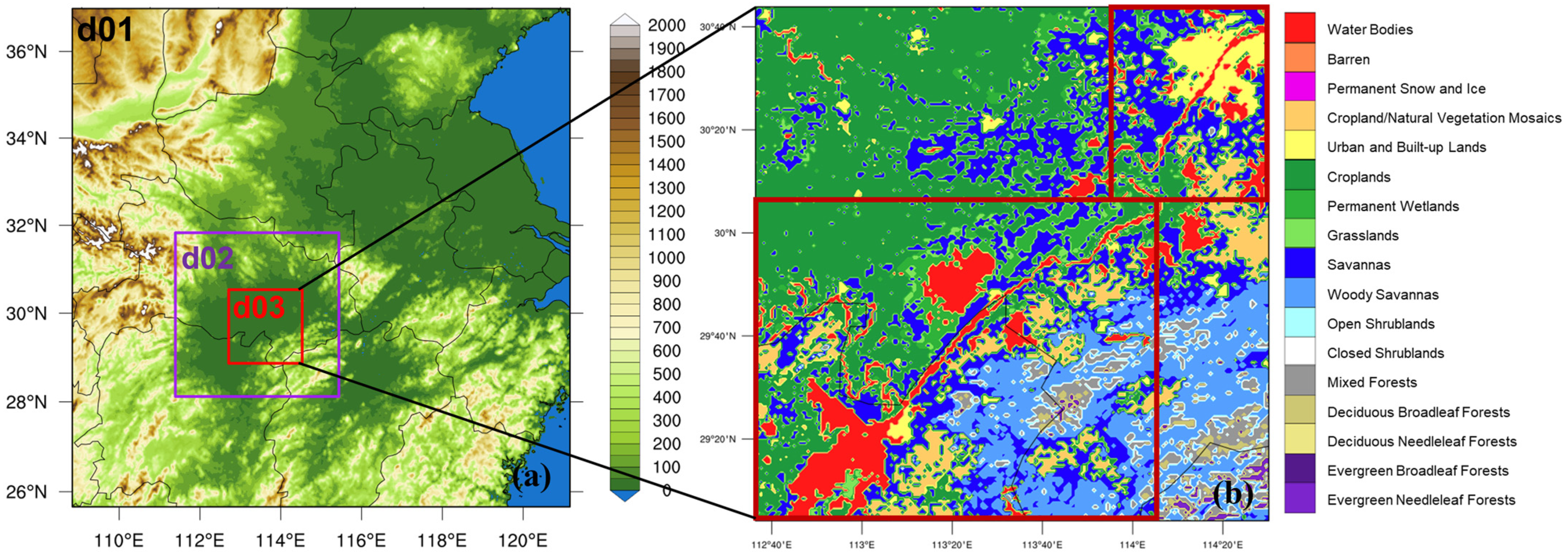
2.2. Model Setting
2.3. Methods of Statistical Analysis
3. Results and Analysis
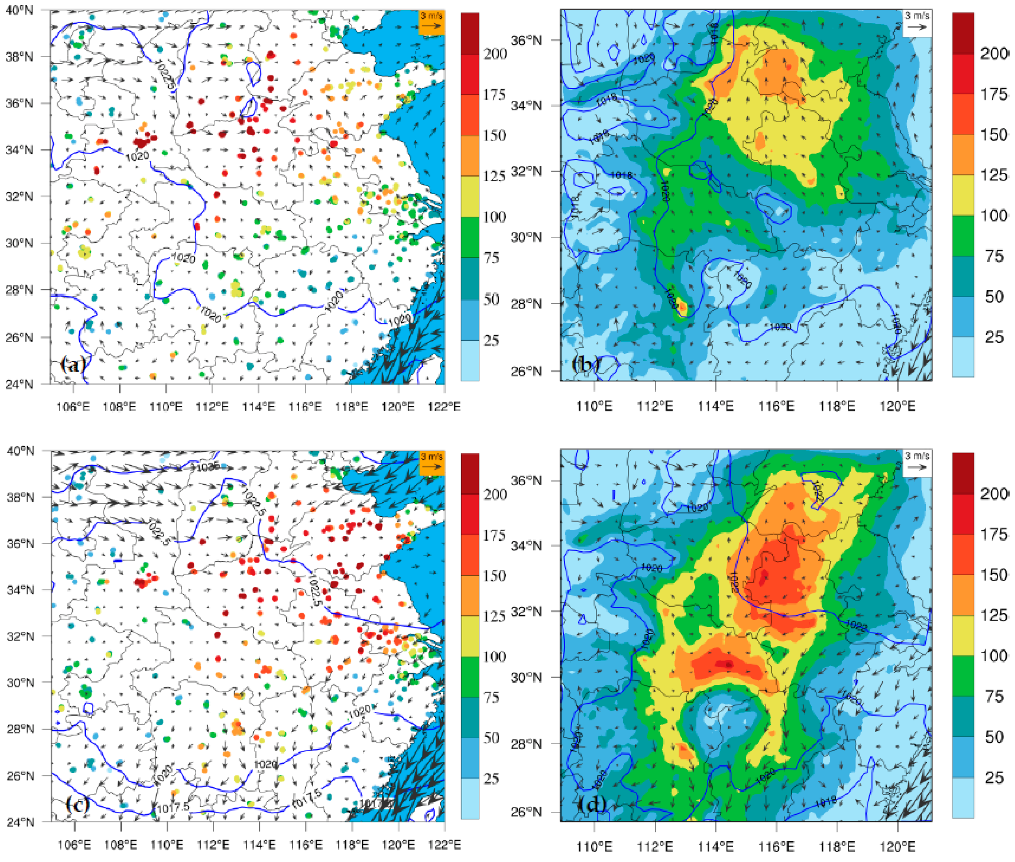
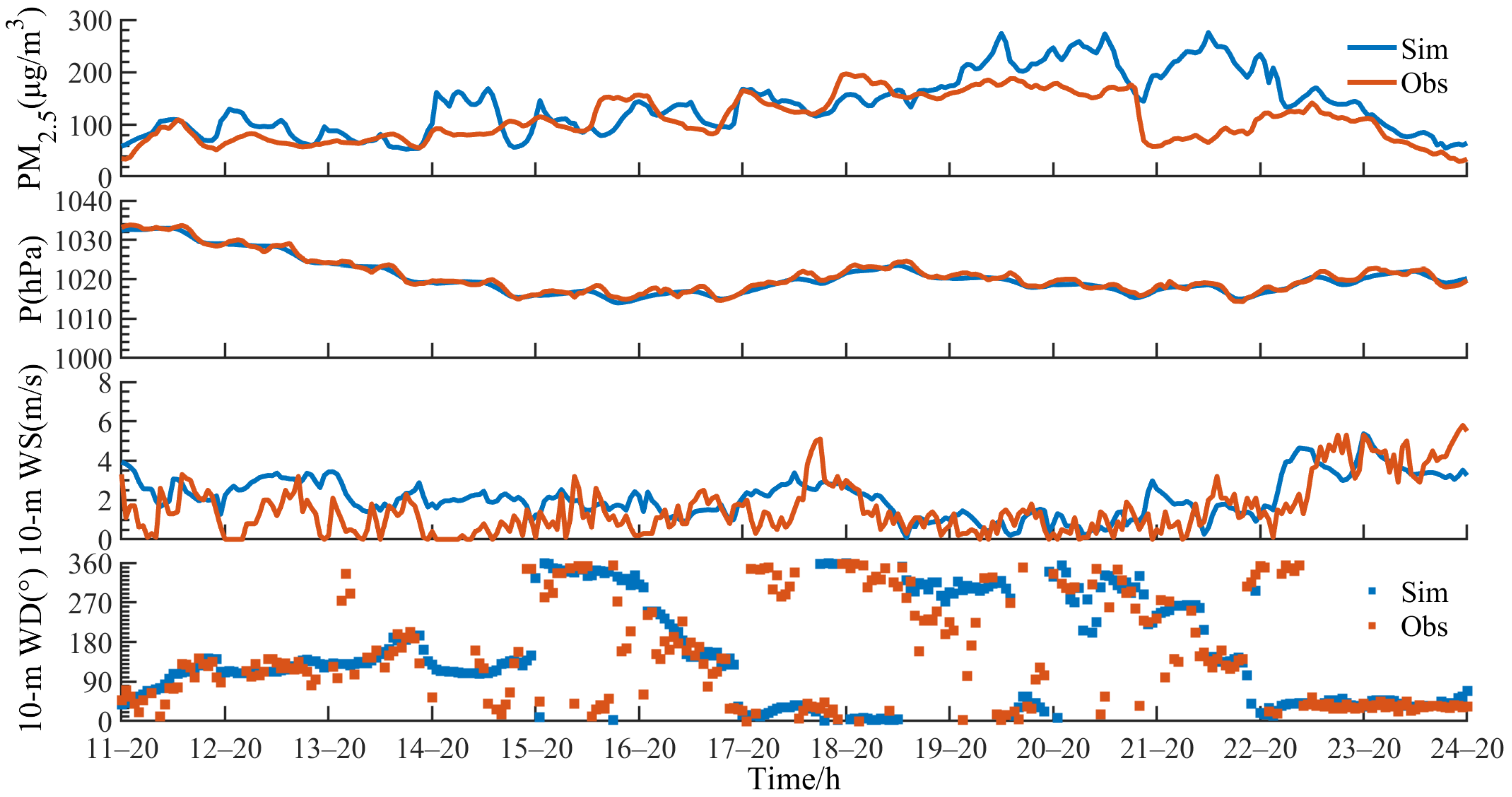
3.1. Simulation and Verification of Heavy Pollution Process
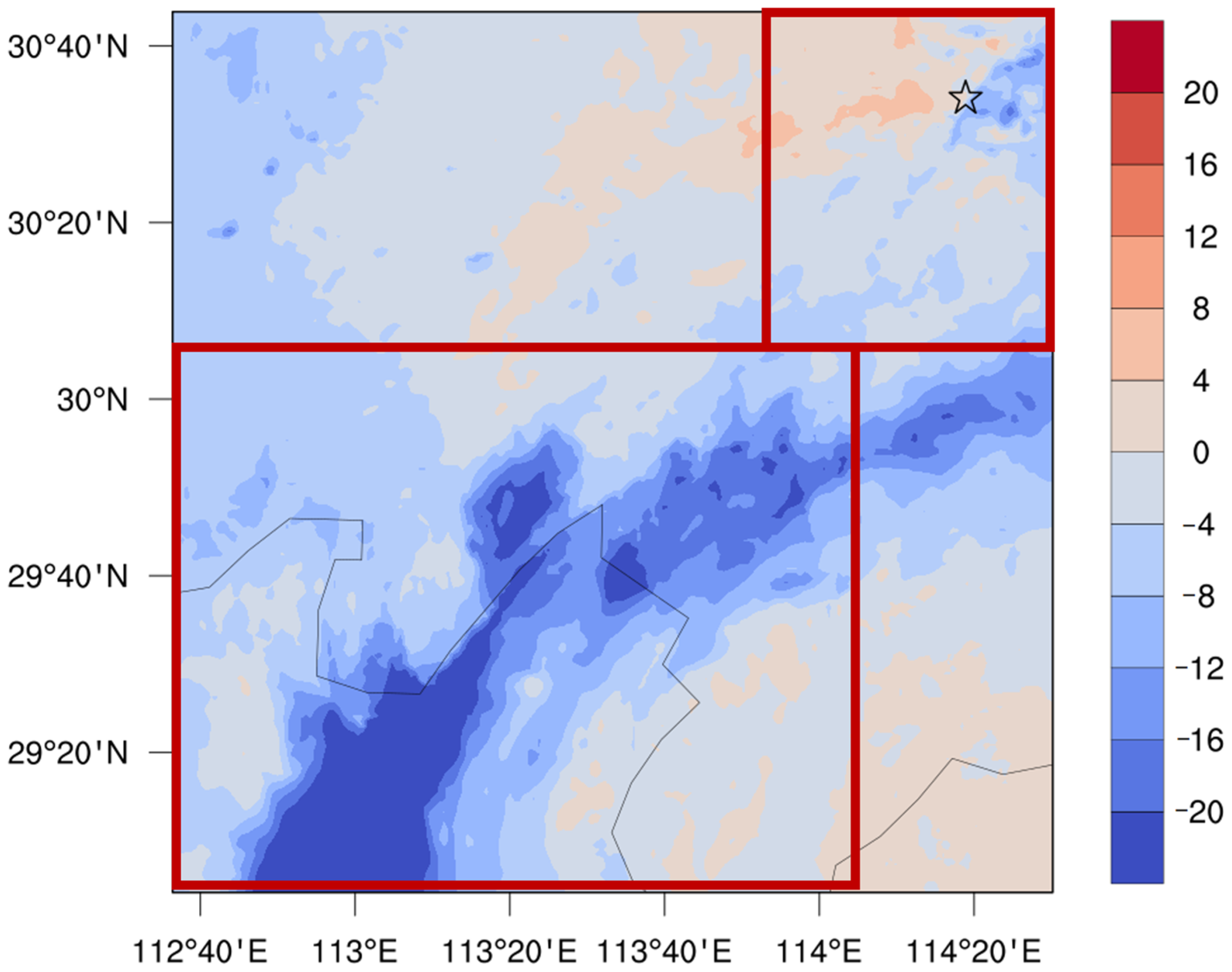
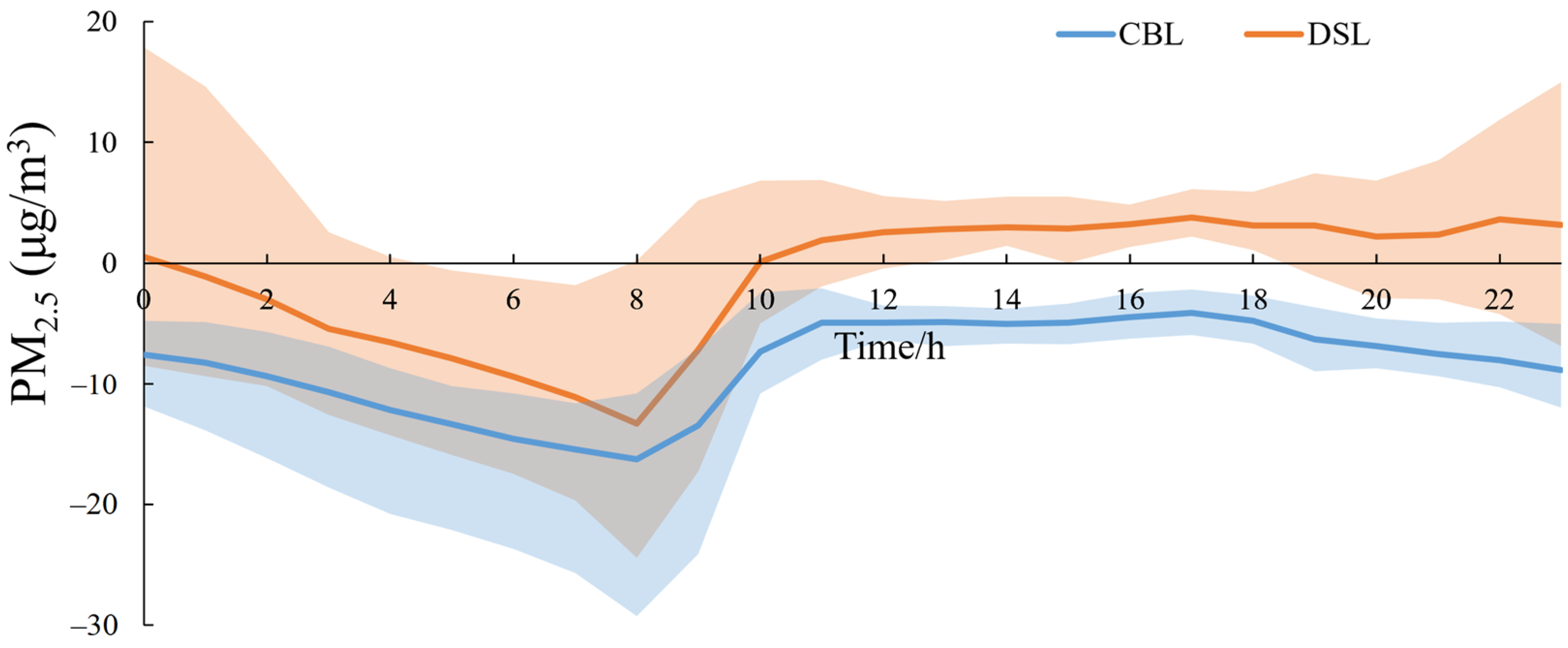
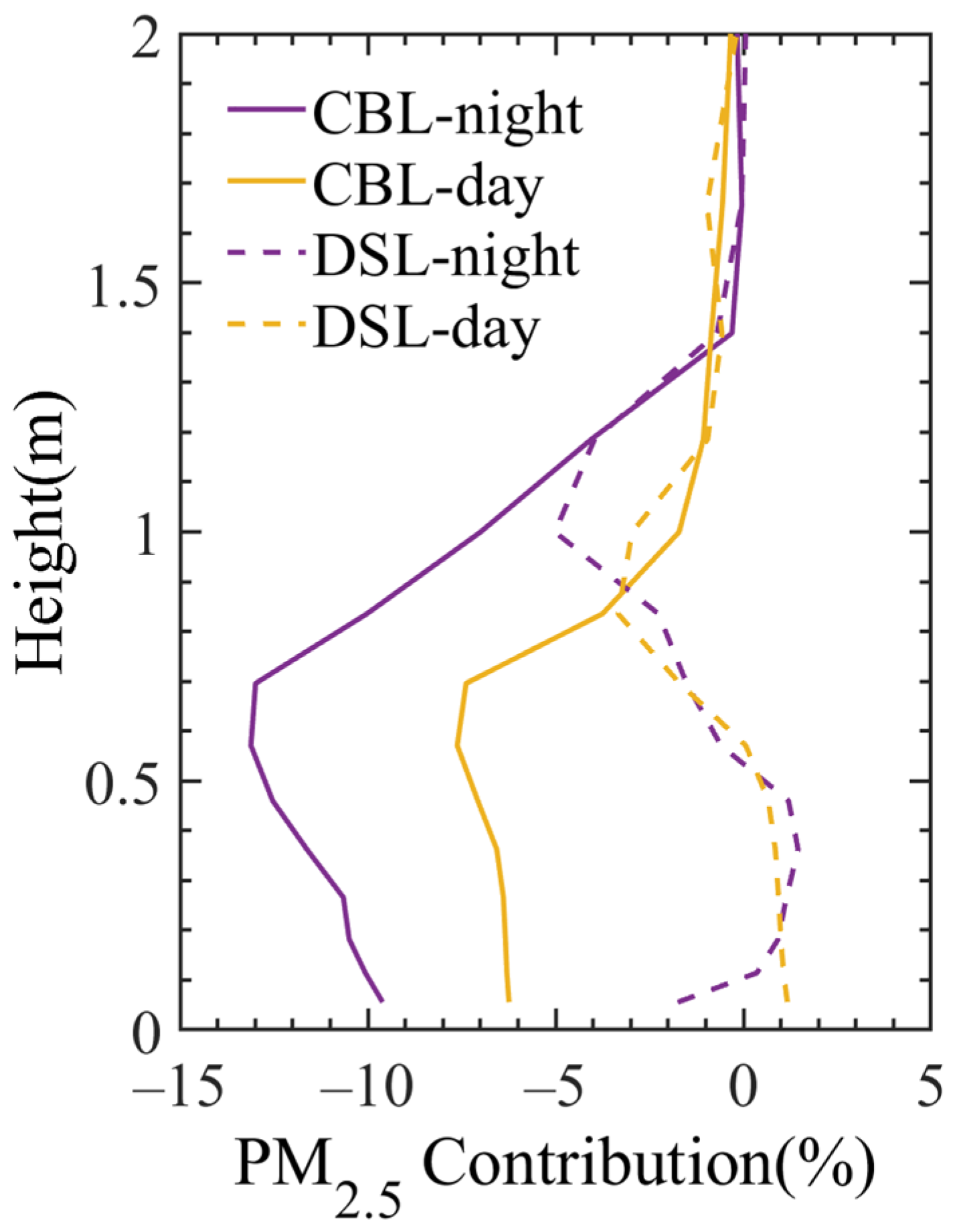
3.2. Influence of Dense “Water Network” on PM2.5 Concentrations
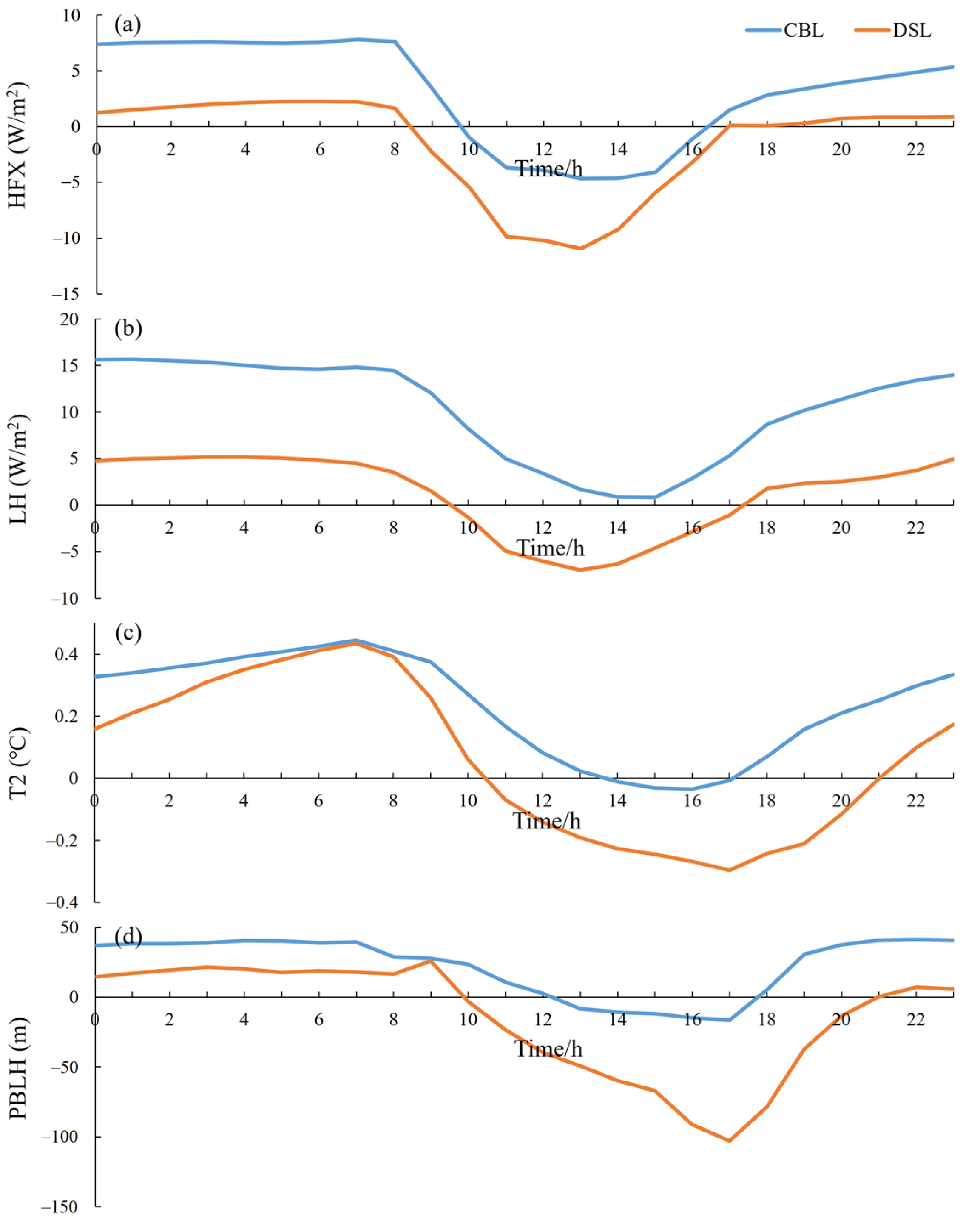
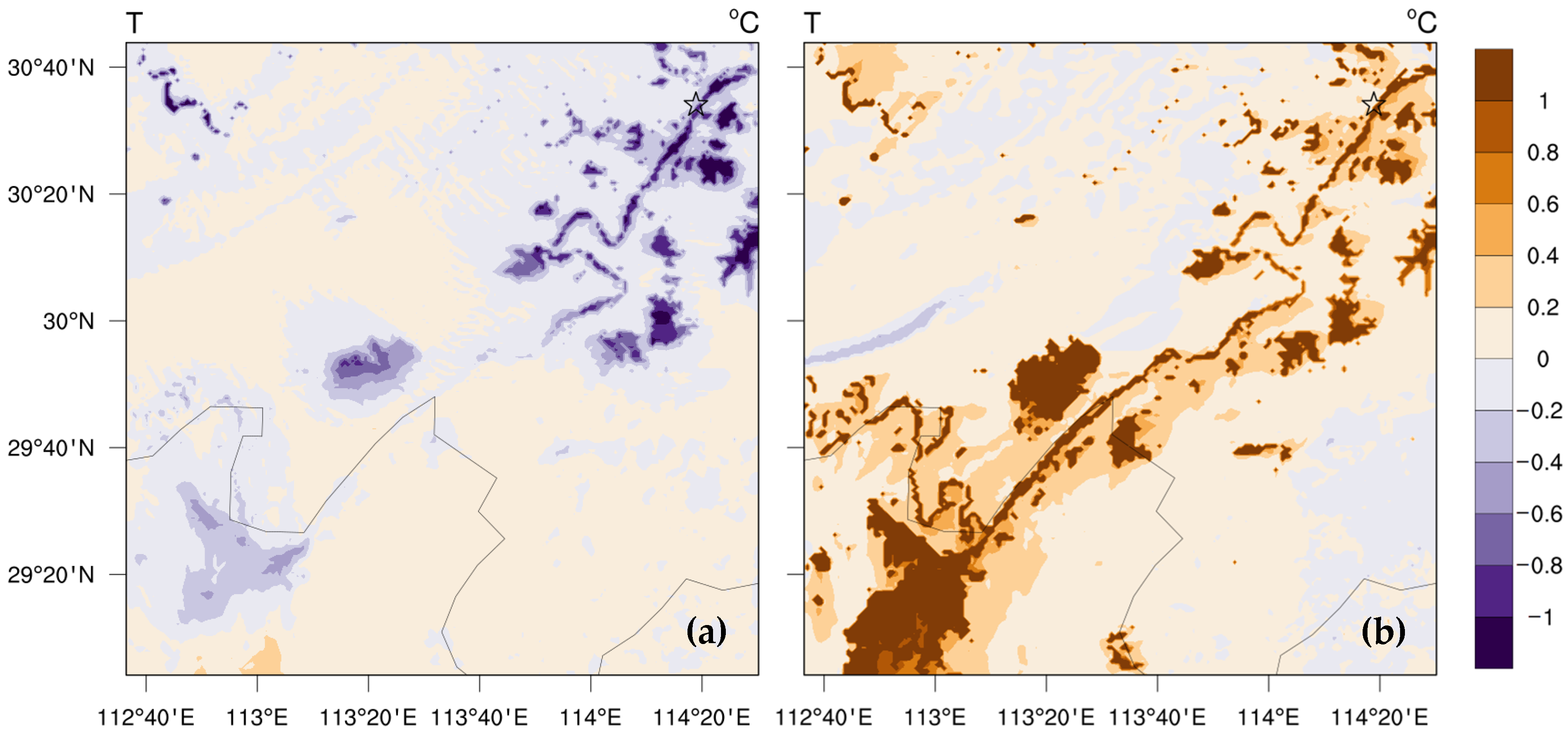
3.3. Influence Mechanism of Dense “Water Network” on Atmospheric Environment
4. Conclusions
Supplementary Materials
Author Contributions
Funding
Institutional Review Board Statement
Informed Consent Statement
Data Availability Statement
Conflicts of Interest
References
- Scott, R.W.; Huff, F.A. Impacts of the Great Lakes on Regional Climate Conditions. J. Great Lakes Res. 1996, 22, 845–863. [Google Scholar] [CrossRef]
- Long, Z.; Perrie, W.; Gyakum, J.; Caya, D.; Laprise, R. Northern Lake Impacts on Local Seasonal Climate. J. Hydrometeorol. 2007, 8, 881–896. [Google Scholar] [CrossRef]
- Thiery, W.; Davin, E.L.; Panitz, H.J.; Demuzere, M.; Lhermitte, S.; van Lipzig, N. The Impact of the African Great Lakes on the Regional Climate. J. Clim. 2015, 28, 4061–4085. [Google Scholar] [CrossRef]
- Wen, L.; Lv, S.; Li, Z.; Zhao, L.; Nagabhatla, N. Impacts of the Two Biggest Lakes on Local Temperature and Precipitation in the Yellow River Source Region of the Tibetan Plateau. Adv. Meteorol. 2015, 2015, 248031. [Google Scholar] [CrossRef]
- Wentworth, G.R.; Murphy, J.G.; Sills, D.M.L. Impact of Lake Breezes on Ozone and Nitrogen Oxides in the Greater Toronto Area. Atmos. Environ. 2015, 109, 52–60. [Google Scholar] [CrossRef]
- Diallo, I.; Giorgi, F.; Stordal, F. Influence of Lake Malawi on Regional Climate from a Double-Nested Regional Climate Model Experiment. Clim. Dyn. 2018, 50, 3397–3411. [Google Scholar] [CrossRef]
- Li, Z.; Lyu, S.; Wen, L.; Zhao, L.; Ao, Y.; Wang, S. Effect of a Cold, Dry Air Incursion on Atmospheric Boundary Layer Processes over a High-Altitude Lake in the Tibetan Plateau. Atmos. Res. 2017, 185, 32–43. [Google Scholar] [CrossRef]
- Su, D.; Wen, L.; Gao, X.; Leppäranta, M.; Song, X.; Shi, Q.; Kirillin, G. Effects of the Largest Lake of the Tibetan Plateau on the Regional Climate. J. Geophys. Res. Atmos. 2020, 125, e2020JD033396. [Google Scholar] [CrossRef]
- Fu, M. Research on the Impacts of Poyang Lake on Typical Weather Process and the Characteristics of near Surface Boundary Layer. Ph.D. Thesis, Nanjing University of Information Science and Technology, Nanjing, China, 2013. [Google Scholar]
- Ren, X.; Wang, Y.; Zhang, Z.; Yang, Y.; Hu, C.; Kang, H. Simulation Studies for Lake Taihu Effect on Surrounding Cities Thermal Environment. Acta Meteorol. Sin. 2017, 75, 645–660. [Google Scholar] [CrossRef]
- Ding, Y.; Liu, Y. Analysis of Long-Term Variations of Fog and Haze in China in Recent 50 Years and Their Relations with Atmospheric Humidity. Sci. China Earth Sci. 2014, 57, 36–46. [Google Scholar] [CrossRef]
- Lai, S.; Zhao, Y.; Ding, A.; Zhang, Y.; Song, T.; Zheng, J.; Ho, K.F.; Lee, S.; Zhong, L. Characterization of PM2.5 and the Major Chemical Components during a 1-Year Campaign in Rural Guangzhou, Southern China. Atmos. Res. 2016, 167, 208–215. [Google Scholar] [CrossRef]
- Lu, D.; Mao, W.; Yang, D.; Zhao, J.; Xu, J. Effects of Land Use and Landscape Pattern on PM2.5 in Yangtze River Delta, China. Atmos. Pollut. Res. 2018, 9, 705–713. [Google Scholar] [CrossRef]
- Zhu, C.; Zeng, Y. Effects of Urban Lake Wetlands on the Spatial and Temporal Distribution of Air PM10 and PM2.5 in the Spring in Wuhan. Urban For. Urban Green. 2018, 31, 142–156. [Google Scholar] [CrossRef]
- Sun, W.; Liu, Z.; Zhang, Y.; Xu, W.; Lv, X.; Liu, Y.; Lyu, H.; Li, X.; Xiao, J.; Ma, F. Study on Land-Use Changes and Their Impacts on Air Pollution in Chengdu. Atmosphere 2019, 11, 42. [Google Scholar] [CrossRef]
- Haurwitz, B. Comments on the Sea-Breeze Circulation. J. Atmos. Sci. 1947, 4, 1–8. [Google Scholar] [CrossRef]
- Lyons, W.A. The Climatology and Prediction of the Chicago Lake Breeze. J. Appl. Meteorol. Climatol. 1972, 11, 1259–1270. [Google Scholar] [CrossRef]
- Physick, W.L. Numerical Experiments on the Inland Penetration of the Sea Breeze. Q. J. R. Met. Soc. 1980, 106, 735–746. [Google Scholar] [CrossRef]
- Liu, J.; Zhu, L.; Wang, H.; Yang, Y.; Liu, J.; Qiu, D.; Ma, W.; Zhang, Z.; Liu, J. Dry Deposition of Particulate Matter at an Urban Forest, Wetland and Lake Surface in Beijing. Atmos. Environ. 2016, 125, 178–187. [Google Scholar] [CrossRef]
- Keen, C.S.; Lyons, W.A. Lake/Land Breeze Circulations on the Western Shore of Lake Michigan. J. Appl. Meteorol. Climatol. 1978, 17, 1843–1855. [Google Scholar] [CrossRef]
- Wang, F.; Wang, Y.; Gao, S.; Hu, N. Simulation Analysis of the Influence of Lake-Land Breeze Circulation on High Ozone Concentration Events. Acta Sci. Circumstantiae 2019, 39, 1392–1401. [Google Scholar]
- Zhao, F.; Zhou, Y.; Xu, H.; Zhu, G.; Zhan, X.; Zou, W.; Zhu, M.; Kang, L.; Zhao, X. Oxic Urban Rivers as a Potential Source of Atmospheric Methane. Environ. Pollut. 2022, 297, 118769. [Google Scholar] [CrossRef] [PubMed]
- Keeler, J.M.; Kristovich, D.A.R. Observations of Urban Heat Island Influence on Lake-Breeze Frontal Movement. J. Appl. Meteorol. Climatol. 2012, 51, 702–710. [Google Scholar] [CrossRef]
- Wu, J.; Li, J.; Peng, J.; Li, W.; Xu, G.; Dong, C. Applying Land Use Regression Model to Estimate Spatial Variation of PM₂.₅ in Beijing, China. Env. Sci. Pollut. Res. Int. 2015, 22, 7045–7061. [Google Scholar] [CrossRef] [PubMed]
- Fu, X.; Wang, X.; Hu, Q.; Li, G.; Ding, X.; Zhang, Y.; He, Q.; Liu, T.; Zhang, Z.; Yu, Q.; et al. Changes in Visibility with PM2.5 Composition and Relative Humidity at a Background Site in the Pearl River Delta Region. J. Environ. Sci. 2016, 40, 10–19. [Google Scholar] [CrossRef]
- Li, G.; Hao, Y.; Yang, T.; Xiao, W.; Pan, M.; Huo, S.; Lyu, T. Enhancing Bioenergy Production from the Raw and Defatted Microalgal Biomass Using Wastewater as the Cultivation Medium. Bioengineering 2022, 9, 637. [Google Scholar] [CrossRef]
- Grell, G.A.; Peckham, S.E.; Schmitz, R.; McKeen, S.A.; Frost, G.; Skamarock, W.C.; Edere, B. Fully coupled “online” chemistry within the WRF model. Atmos. Environ. 2005, 39, 6957–6975. [Google Scholar] [CrossRef]
- Sha, T.; Ma, X.; Wang, J.; Tian, R.; Zhao, J.; Cao, F.; Zhang, Y.L. Improvement of inorganic aerosol component in PM2.5 by constraining aqueous-phase formation of sulfate in cloud with satellite retrievals: WRF-Chem simulations. Sci. Total Environ. 2022, 804, 150229. [Google Scholar] [CrossRef]
- Gustafson, W.I.; Chapman, E.G.; Ghan, S.J.; Easter, R.C.; Fast, J.D. Impact on modeled cloud characteristics due to simplified treatment of uniform cloud condensation nuclei during NEAQS 2004. Geophys. Res. Lett. 2007, 34, 255–268. [Google Scholar] [CrossRef]
- Guo, J.; He, J.; Liu, H.; Miao, Y.; Liu, H.; Zhai, P. Impact of various emission control schemes on air quality using WRF-Chem during APEC China 2014. Atmos. Environ. 2016, 140, 311–319. [Google Scholar] [CrossRef]
- Lennartson, E.M.; Wang, J.; Gu, J.; Garcia, L.C.; Ge, C.; Gao, M.; Choi, M.; Saide, P.; Carmichael, G.R.; Kim, J.; et al. Diurnal variation of aerosol optical depth and PM2.5 in South Korea: A synthesis from AERONET, satellite (GOCI), KORUS-AQ observation, and the WRF-Chem model. Atmos. Chem. Phys. 2018, 18, 15125–15144. [Google Scholar] [CrossRef]
- Liang, C.; Zhang, X.; Li, Z.; Xiao, Y. Temporal and Spatial Evolution Characteristics of River and Lake Systems in the Urbanization Process of Wuhan City. J. North China Univ. Water Resour. Electr. Power 2019, 40, 61–68. [Google Scholar] [CrossRef]
- Shen, L.; Wang, H.; Zhao, T.; Liu, J.; Bai, Y.; Kong, S.; Shu, Z. Characterizing Regional Aerosol Pollution in Central China Based on 19 Years of MODIS Data: Spatiotemporal Variation and Aerosol Type Discrimination. Environ. Pollut. 2020, 263, 114556. [Google Scholar] [CrossRef]
- Yu, C.; Zhao, T.; Bai, Y.; Zhang, L.; Kong, S.; Yu, X.; He, J.; Cui, C.; Yang, J.; You, Y.; et al. Heavy Air Pollution with a Unique “Non-Stagnant” Atmospheric Boundary Layer in the Yangtze River Middle Basin Aggravated by Regional Transport of PM2.5 over China. Atmos. Chem. Phys. 2020, 20, 7217–7230. [Google Scholar] [CrossRef]
- Zhu, Y.; Zhao, T.; Bai, Y.; Xu, J.; Sun, X.; Hu, W.; Chang, J.; Yang, J.; Zhu, C. Characteristics of Atmospheric Particulate Matter Pollution and the Unique Wind and Underlying Surface Impact in the Twain-Hu Basin in Winter. Environ. Sci. 2021, 42, 4669–4677. [Google Scholar] [CrossRef]
- Lin, C.; Chen, F.; Huang, J.C.; Chen, W.C.; Liou, Y.A.; Chen, W.N.; Liu, S.C. Urban Heat Island Effect and Its Impact on Boundary Layer Development and Land–Sea Circulation over Northern Taiwan. Atmos. Environ. 2008, 42, 5635–5649. [Google Scholar] [CrossRef]
- Blanken, P.D.; Spence, C.; Hedstrom, N.; Lenters, J.D. Evaporation from Lake Superior: 1. Physical Controls and Processes. J. Great Lakes Res. 2011, 37, 707–716. [Google Scholar] [CrossRef]
- Hou, P.; Chen, Y.; Qiao, W.; Cao, G.; Jiang, W.; Li, J. Near-Surface Air Temperature Retrieval from Satellite Images and Influence by Wetlands in Urban Region. Appl. Clim. 2013, 111, 109–118. [Google Scholar] [CrossRef]
- Hu, X.; Xue, M. Influence of Synoptic Sea-Breeze Fronts on the Urban Heat Island Intensity in Dallas–Fort Worth, Texas. Mon. Weather. Rev. 2016, 144, 1487–1507. [Google Scholar] [CrossRef]
- Zhu, C.; Przybysz, A.; Chen, Y.; Guo, H.; Chen, Y.; Zeng, Y. Effect of Spatial Heterogeneity of Plant Communities on Air PM10 and PM2.5 in an Urban Forest Park in Wuhan, China. Urban For. Urban Green. 2019, 46, 126487. [Google Scholar] [CrossRef]
- Li, M.; Zhang, Q.; Kurokawa, J.I.; Woo, J.H.; He, K.; Lu, Z.; Ohara, T.; Song, Y.; Streets, D.G.; Carmichael, G.R.; et al. MIX: A Mosaic Asian Anthropogenic Emission Inventory under the International Collaboration Framework of the MICS-Asia and HTAP. Atmos. Chem. Phys. 2017, 17, 935–963. [Google Scholar] [CrossRef]
- Qi, J.; Zheng, B.; Li, M.; Yu, F.; Chen, C.; Liu, F.; Zhou, X.; Yuan, J.; Zhang, Q.; He, K. A High-Resolution Air Pollutants Emission Inventory in 2013 for the Beijing-Tianjin-Hebei Region, China. Atmos. Environ. 2017, 170, 156–168. [Google Scholar] [CrossRef]
- Lin, Y.L.; Farley, R.D.; Orville, H.D. Bulk Parameterization of the Snow Field in a Cloud Model. J. Appl. Meteorol. Climatol. 1983, 22, 1065–1092. [Google Scholar] [CrossRef]
- Mlawer, E.J.; Taubman, S.J.; Brown, P.D.; Iacono, M.J.; Clough, S.A. Radiative Transfer for Inhomogeneous Atmospheres: RRTM, a Validated Correlated-k Model for the Longwave. J. Geophys. Res. 1997, 102, 16663–16682. [Google Scholar] [CrossRef]
- Chou, M.D.; Suarez, M.J.; Ho, C.H.; Yan, M.M.H.; Lee, K.T. Parameterizations for Cloud Overlapping and Shortwave Single-Scattering Properties for Use in General Circulation and Cloud Ensemble Models. J. Clim. 1998, 11, 202–214. [Google Scholar] [CrossRef]
- Tewari, M.; Wang, W.; Dudhia, J.; LeMone, M.A.; Mitchell, K.; Ek, M.; Gayno, G.; Wegiel, J.; Cuenca, R. Implementation and Verification of the United NOAH Land Surface Model in the WRF Model. In Proceedings of the 20th Conference on Weather Analysis and Forecasting/16th Conference on Numerical Weather Prediction, Seattle, WA, USA, 10–12 January 2004; p. 15. [Google Scholar]
- Gu, H.; Jin, J.; Wu, Y.; Ek, M.B.; Subin, Z.M. Calibration and Validation of Lake Surface Temperature Simulations with the Coupled WRF-Lake Model. Clim. Chang. 2015, 129, 471–483. [Google Scholar] [CrossRef]
- Gu, H.; Shen, X.; Jin, J.; Zhao, L.; Xiao, W.; Wang, Y. Evaluation on Simulation of Coupled WRF Lake Model to Lake Surface Temperature in Taihu Lake. Meteorol. Mon. 2014, 40, 166–173. [Google Scholar] [CrossRef]
- Boylan, J.W.; Russell, A.G. PM and Light Extinction Model Performance Metrics, Goals, and Criteria for Three-Dimensional Air Quality Models. Atmos. Environ. 2006, 40, 4946–4959. [Google Scholar] [CrossRef]
- Astrup, P.; Mikkelsen, T.K. Comparison of NWP Prognosis and Local Monitoring Data from NPPs. Radioprotection 2010, 45, S97–S111. [Google Scholar] [CrossRef]
- Huang, A.; Lazhu; Wang, J.; Dai, Y.; Yang, K.; Wei, N.; Wen, L.; Wu, Y.; Zhu, X.; Zhang, X.; et al. Evaluating and Improving the Performance of Three 1-D Lake Models in a Large Deep Lake of the Central Tibetan Plateau. J. Geophys. Res. Atmos. 2019, 124, 3143–3167. [Google Scholar] [CrossRef]
- Wang, T.; Huang, X.; Wang, Z.; Liu, Y.; Zhou, D.; Ding, K.; Wang, H.; Qi, X.; Ding, A. Secondary Aerosol Formation and Its Linkage with Synoptic Conditions during Winter Haze Pollution over Eastern China. Sci. Total Environ. 2020, 730, 138888. [Google Scholar] [CrossRef]
- Nie, W.; Yan, C.; Huang, D.D.; Wang, Z.; Liu, Y.; Qiao, X.; Guo, Y.; Tian, L.; Zheng, P.; Xu, Z.; et al. Secondary Organic Aerosol Formed by Condensing Anthropogenic Vapours over China’s Megacities. Nat. Geosci. 2022, 15, 255–261. [Google Scholar] [CrossRef]


| Station | Variables | R | RMSE | MB | GE | MFB (%) | MFE (%) |
|---|---|---|---|---|---|---|---|
| Wuhan | 2-m temperature (°C) | 0.78 ** | 3.88 | 3.11 | 3.25 | 47.33 | 49.42 |
| 2-m relative humidity (%) | 0.71 ** | 26.43 | −23.34 | 23.37 | −20.94 | 20.97 | |
| 10-m wind speed (m/s) | 0.57 ** | 1.28 | 0.56 | 1.03 | 44.83 | 59.11 | |
| 10-m wind direction (°) | 0.27** | 139.65 | −5.68 | 83.88 | 9.20 | 39.95 | |
| Surface air pressure (hPa) | 0.99 ** | 0.88 | −0.46 | 0.71 | −0.03 | 0.05 | |
| Precipitation rate (mm/h) | 0.60 ** | 0.14 | 0.00 | 0.04 | / | / | |
| Near-surface PM25 (μg/m3) | 0.56 ** | 56.34 | 28.68 | 38.99 | 16.41 | 22.03 | |
| Yueyang | 2-m temperature (°C) | 0.80 ** | 3.58 | 3.32 | 3.32 | 33.26 | 33.29 |
| 2-m relative humidity (%) | 0.82 ** | 16.44 | −12.69 | 14.18 | −10.14 | 12.14 | |
| 10-m wind speed (m/s) | 0.64 ** | 2.41 | 1.88 | 2.05 | 50.45 | 55.39 | |
| 10-m wind direction (°) | 0.41** | 117.98 | −8.36 | 71.31 | 9.34 | 42.92 | |
| Surface air pressure (hPa) | 0.99 ** | 1.49 | 1.30 | 1.32 | 0.09 | 0.09 | |
| Precipitation rate (mm/h) | 0.70 ** | 0.21 | −0.02 | 0.09 | / | / | |
| Near-surface PM25 (μg/m3) | 0.31 ** | 42.70 | 1.86 | 35.63 | 5.15 | 26.78 |
| Variables | CBL | DSL |
|---|---|---|
| Sensible heat flux | −0.35 ** | −0.47 ** |
| Latent heat flux | −0.37 ** | −0.57 ** |
| 2-m temperature | −0.64 ** | −0.75 ** |
| 2-m relative humidity | 0.54 ** | −0.08 |
| Atmospheric boundary layer height | −0.40 ** | −0.52 ** |
| 10-m wind speed | 0.01 | −0.40 ** |
| Variables | CBLs | DSLs |
|---|---|---|
| Sensible heat flux | 13.65% | 16.17% |
| Latent heat flux | 29.14% | 21.96% |
| 2-m temperature | 38.83% | 49.79% |
| 2-m relative humidity | 14.77% | 5.35% |
| Atmospheric boundary layer height | 0.87% | 2.18% |
| 10-m wind speed | 2.75% | 4.54% |
Disclaimer/Publisher’s Note: The statements, opinions and data contained in all publications are solely those of the individual author(s) and contributor(s) and not of MDPI and/or the editor(s). MDPI and/or the editor(s) disclaim responsibility for any injury to people or property resulting from any ideas, methods, instructions or products referred to in the content. |
© 2023 by the authors. Licensee MDPI, Basel, Switzerland. This article is an open access article distributed under the terms and conditions of the Creative Commons Attribution (CC BY) license (https://creativecommons.org/licenses/by/4.0/).
Share and Cite
Zhu, Y.; Bai, Y.; Xiong, J.; Zhao, T.; Xu, J.; Zhou, Y.; Meng, K.; Meng, C.; Sun, X.; Hu, W. Mitigation Effect of Dense “Water Network” on Heavy PM2.5 Pollution: A Case Model of the Twain-Hu Basin, Central China. Toxics 2023, 11, 169. https://doi.org/10.3390/toxics11020169
Zhu Y, Bai Y, Xiong J, Zhao T, Xu J, Zhou Y, Meng K, Meng C, Sun X, Hu W. Mitigation Effect of Dense “Water Network” on Heavy PM2.5 Pollution: A Case Model of the Twain-Hu Basin, Central China. Toxics. 2023; 11(2):169. https://doi.org/10.3390/toxics11020169
Chicago/Turabian StyleZhu, Yan, Yongqing Bai, Jie Xiong, Tianliang Zhao, Jiaping Xu, Yue Zhou, Kai Meng, Chengzhen Meng, Xiaoyun Sun, and Weiyang Hu. 2023. "Mitigation Effect of Dense “Water Network” on Heavy PM2.5 Pollution: A Case Model of the Twain-Hu Basin, Central China" Toxics 11, no. 2: 169. https://doi.org/10.3390/toxics11020169
APA StyleZhu, Y., Bai, Y., Xiong, J., Zhao, T., Xu, J., Zhou, Y., Meng, K., Meng, C., Sun, X., & Hu, W. (2023). Mitigation Effect of Dense “Water Network” on Heavy PM2.5 Pollution: A Case Model of the Twain-Hu Basin, Central China. Toxics, 11(2), 169. https://doi.org/10.3390/toxics11020169