
Local Scale Exposure and Fate of Engineered Nanomaterials


Abstract
: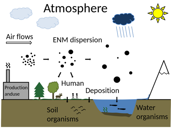
1. Introduction
2. Materials and Methods
2.1. Atmospheric Dispersion and Deposition Model
2.1.1. Gaussian Plume Formulation
2.1.2. Nanomaterial Deposition Calculation
2.1.3. Boundary Layer Reflection
2.1.4. Mass Balance Correction
2.2. Division between Local and Regional Environments
2.3. Simulation of the Maximal Range of Distances
2.4. Case Study Simulations of TiO Environmental Releases
3. Results
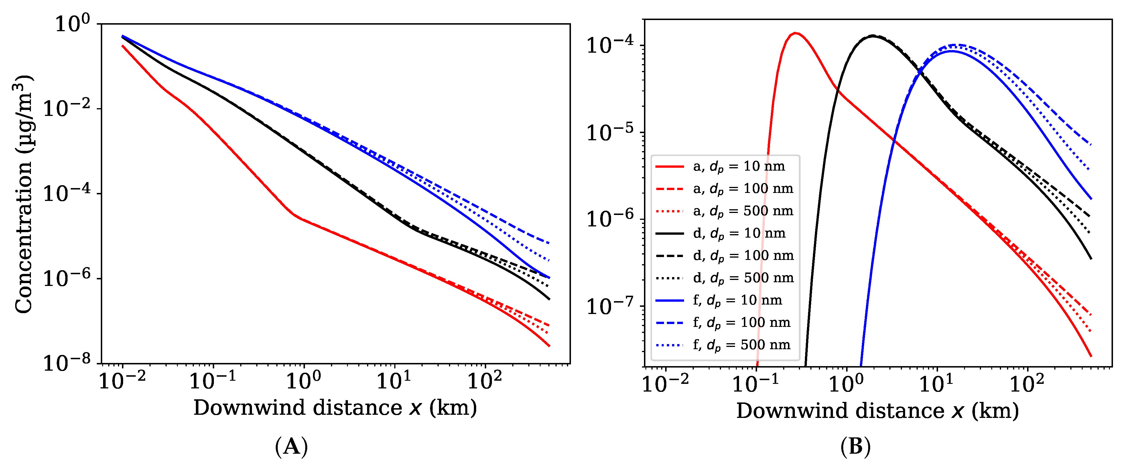
3.1. Ground Level Concentrations
3.2. Maximum Ground Level Concentrations and Associated Distances
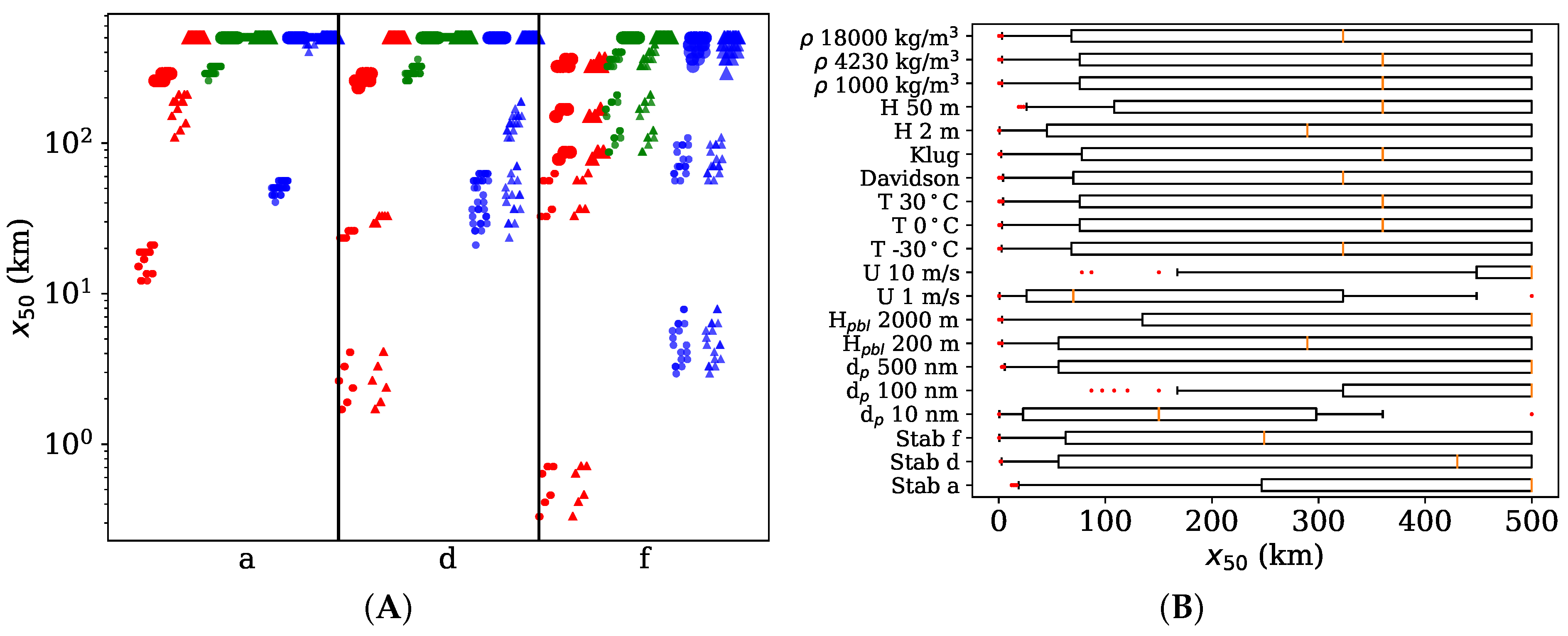
3.3. Distance of 50% Deposited
3.4. Case Study Simulations of TiO Environmental Releases
3.5. Comparison of Dispersion to Fully Mixed Compartments
4. Discussion
4.1. Local Scale of Exposure Estimation
4.2. Implications for Nanomaterial Environmental Exposure and Fate Assessment
4.3. Applicability to Other Atmospheric Pollutants
4.4. Implications for Chemical Regulations
4.5. Atmospheric Release of TiO as a Case for ENM Exposure Assessment
4.6. Implications for Occupational Exposure Assessment
4.7. Implications for Public Health
4.8. Limitations and Further Studies
5. Conclusions
Supplementary Materials
Author Contributions
Funding
Institutional Review Board Statement
Informed Consent Statement
Data Availability Statement
Acknowledgments
Conflicts of Interest
Abbreviations
| ADiDeNano | Atmospheric Dispersion and Deposition model developed in this study |
| CFD | Computational fluid dynamics |
| CNT | Carbon nanotubes |
| EC-TGD | European Commission Technical Guidance Document on risk assessment |
| ENM | Engineered nanomaterial |
| EPA | Environmental Protection Agency (U.S.) |
| EUSES | European Union System for the Evaluation of Substances |
| FF | Far field |
| FOCUS | FOrum for Co-ordination of pesticide fate models and their USe |
| MAFOR | Multicomponent Aerosol FORmation model |
| NF | Near field |
| OEL | Occupational exposure limit |
| OPS | Operational Priority Substances model |
| PBL | Planetary boundary layer |
| PM | Particulate matter - mass concentration of particles below 2.5 m in diameter |
| Predicted environmental concentration | |
| Local predicted environmental concentration | |
| Regional predicted environmental concentration | |
| Predicted environmental concentration in soil | |
| Predicted no effect concentration | |
| Predicted no effect concentration in soil | |
| REACH | Registration, Evaluation, Authorisation and Restriction of Chemicals in Europe |
| REL | Recommended exposure limit |
| SB4N | SimpleBox4nano—multimedia nanomaterial exposure and fate assessment model |
| TiO | Titanium dioxide |
| WHO | World Health Organization |
Appendix A. Gaussian Solutions
Appendix A.1. Ermak’s Solution for Deposition
Appendix A.2. Yamartino’s Solution for Boundary Layer Reflection
Appendix B. Derivation of a Simple Mass Balance Model for Local and Regional Compartments

References
- Holmes, N.S.; Morawska, L. A review of dispersion modelling and its application to the dispersion of particles: An overview of different dispersion models available. Atmos. Environ. 2006, 40, 5902–5928. [Google Scholar] [CrossRef] [Green Version]
- Karl, M.; Gross, A.; Pirjola, L.; Leck, C. A new flexible multicomponent model for the study of aerosol dynamics in the marine boundary layer. Tellus Chem. Phys. Meteorol. 2011, 63, 1001–1025. [Google Scholar] [CrossRef] [Green Version]
- Karl, M.; Wright, R.F.; Berglen, T.F.; Denby, B. Worst case scenario study to assess the environmental impact of amine emissions from a CO2 capture plant. Int. J. Greenh. Gas Control. 2011, 5, 439–447. [Google Scholar] [CrossRef]
- Karamchandani, P.; Vijayaraghavan, K.; Yarwood, G. Sub-Grid Scale Plume Modeling. Atmosphere 2011, 2, 389. [Google Scholar] [CrossRef] [Green Version]
- Leelossy, Á.; Molnár, F.; Izsák, F.; Havasi, Á.; Lagzi, I.; Mészáros, R. Dispersion modeling of air pollutants in the atmosphere: A review. Open Geosci. 2014, 6, 257–278. [Google Scholar] [CrossRef]
- Keuken, M.P.; Moerman, M.; Zandveld, P.; Henzing, J.S.; Hoek, G. Total and size-resolved particle number and black carbon concentrations in urban areas near Schiphol airport (The Netherlands). Atmos. Environ. 2015, 104, 132–142. [Google Scholar] [CrossRef]
- Keuken, M.P.; Moerman, M.; Zandveld, P.; Henzing, J.S. Total and size-resolved particle number and black carbon concentrations near an industrial area. Atmos. Environ. 2015, 122, 196–205. [Google Scholar] [CrossRef]
- Kukkonen, J.; Karl, M.; Keuken, M.P.; Denier van der Gon, H.A.C.; Denby, B.R.; Singh, V.; Douros, J.; Manders, A.; Samaras, Z.; Moussiopoulos, N.; et al. Modelling the dispersion of particle numbers in five European cities. Geosci. Model Dev. 2016, 9, 451–478. [Google Scholar] [CrossRef] [Green Version]
- Leelossy, Á.; Lagzi, I.; Kovács, A.; Mészáros, R. A review of numerical models to predict the atmospheric dispersion of radionuclides. J. Environ. Radioact. 2018, 182, 20–33. [Google Scholar] [CrossRef]
- John, A.C.; Küpper, M.; Manders-Groot, A.M.M.; Debray, B.; Lacome, J.M.; Kuhlbusch, T.A.J. Emissions and possible environmental implication of engineered nanomaterials (ENMs) in the atmosphere. Atmosphere 2017, 8, 84. [Google Scholar] [CrossRef] [Green Version]
- Fonseca, A.S.; Viitanen, A.K.; Kanerva, T.; Säämänen, A.; Aguerre-Chariol, O.; Fable, S.; Dermigny, A.; Karoski, N.; Fraboulet, I.; Koponen, I.K.; et al. Occupational exposure and environmental release: The case study of pouring TiO2 and filler materials for paint production. Int. J. Environ. Res. Public Health 2021, 18, 418. [Google Scholar] [CrossRef] [PubMed]
- Koivisto, A.J.; Del Secco, B.; Trabucco, S.; Nicosia, A.; Ravegnani, F.; Altin, M.; Cabellos, J.; Furxhi, I.; Blosi, M.; Costa, A.; et al. Quantifying Emission Factors and Setting Conditions of Use According to ECHA Chapter R. 14 for a Spray Process Designed for Nanocoatings—A Case Study. Nanomaterials 2022, 12, 596. [Google Scholar] [CrossRef] [PubMed]
- Nowack, B.; Mueller, N.C.; Krug, H.F.; Wick, P. How to consider engineered nanomaterials in major accident regulations? Environ. Sci. Eur. 2014, 26, 1–10. [Google Scholar] [CrossRef] [Green Version]
- Gottschalk, F.; Sonderer, T.; Scholz, R.W.; Nowack, B. Modeled environmental concentrations of engineered nanomaterials (TiO2, ZnO, Ag, CNT, fullerenes) for different regions. Environ. Sci. Technol. 2009, 43, 9216–9222. [Google Scholar] [CrossRef] [PubMed]
- Walser, T.; Schwabe, F.; Thöni, L.; De Temmerman, L.; Hellweg, S. Nanosilver emissions to the atmosphere: A new challenge? E3s Web Conf. 2013, 1, 14003. [Google Scholar] [CrossRef] [Green Version]
- Baalousha, M.; Cornelis, G.; Kuhlbusch, T.A.J.; Lynch, I.; Nickel, C.; Peijnenburg, W.J.G.M.; Van Den Brink, N.W. Modeling nanomaterial fate and uptake in the environment: Current knowledge and future trends. Environ. Sci. Nano 2016, 3, 323–345. [Google Scholar] [CrossRef]
- Hristozov, D.; Gottardo, S.; Semenzin, E.; Oomen, A.; Bos, P.; Peijnenburg, W.; van Tongeren, M.; Nowack, B.; Hunt, N.; Brunelli, A.; et al. Frameworks and tools for risk assessment of manufactured nanomaterials. Environ. Int. 2016, 95, 36–53. [Google Scholar] [CrossRef]
- Nowack, B. Evaluation of environmental exposure models for engineered nanomaterials in a regulatory context. NanoImpact 2017, 8, 38–47. [Google Scholar] [CrossRef]
- Kuhlbusch, T.A.J.; Wijnhoven, S.W.P.; Haase, A. Nanomaterial exposures for worker, consumer and the general public. NanoImpact 2018, 10, 11–25. [Google Scholar] [CrossRef]
- Quik, J.T.K.; Bakker, M.; van de Meent, D.; Poikkimäki, M.; Dal Maso, M.; Peijnenburg, W. Directions in QPPR development to complement the predictive models used in risk assessment of nanomaterials. NanoImpact 2018, 11, 58–66. [Google Scholar] [CrossRef]
- Sørensen, S.N.; Baun, A.; Burkard, M.; Dal Maso, M.; Hansen, S.F.; Harrison, S.; Hjorth, R.; Lofts, S.; Matzke, M.; Nowack, B.; et al. Evaluating environmental risk assessment models for nanomaterials according to requirements along the product innovation Stage-Gate process. Environ. Sci. Nano 2019, 6, 505–518. [Google Scholar] [CrossRef] [Green Version]
- Wigger, H.; Kägi, R.; Wiesner, M.; Nowack, B. Exposure and Possible Risks of Engineered Nanomaterials in the Environment—Current Knowledge and Directions for the Future. Rev. Geophys. 2020, 58, e2020RG000710. [Google Scholar] [CrossRef]
- Meesters, J.A.J.; Koelmans, A.A.; Quik, J.T.K.; Hendriks, A.J.; van de Meent, D. Multimedia modeling of engineered nanoparticles with SimpleBox4nano: Model definition and evaluation. Environ. Sci. Technol. 2014, 48, 5726–5736. [Google Scholar] [CrossRef] [PubMed]
- Manders, A.M.M.; Builtjes, P.J.H.; Curier, L.; Denier van der Gon, H.A.C.; Hendriks, C.; Jonkers, S.; Kranenburg, R.; Kuenen, J.J.P.; Segers, A.J.; Timmermans, R.M.A.; et al. Curriculum vitae of the LOTOS-EUROS (v2.0) chemistry transport model. Geosci. Model Dev. 2017, 10, 4145–4173. [Google Scholar] [CrossRef] [Green Version]
- Quik, J.T.K.; Meesters, J.; Slootweg, J.; Peijnenburg, W.; Harrison, S.; Manders, A.; Kuenen, J.; Adam, V.; Lofts, S. NanoFASE SimpleBox4Nano specifications update. H2020 NanoFASE Project Deliverable 2.5. 2019, Month 49. Available online: https://ec.europa.eu/research/participants/documents/downloadPublic?documentIds=080166e5c9c2be42&appId=PPGMS (accessed on 1 May 2022).
- EC. Technical Guidance Document on Risk Assessment, in Support of Commission Directive 93/67/EEC on Risk Assessment for New Notified Substances; Commission Regulation (EC) No. 1488/94 on Risk Assessment for Existing Substances; Directive 98/8/EC of the European Parliament Council Concerning the Placing of Biocidal Products on the Market. Part I, II, III, IV. European Commission, Joint Research Centre, European Chemicals Bureau, Italy. 2003. Available online: https://op.europa.eu/en/publication-detail/-/publication/d813d6a6-7d3d-41b5-8e80-ac60868ab143/language-en/format-PDF/source-256230411 (accessed on 1 May 2022).
- EC. European Union System for the Evaluation of Substances 2.0 (EUSES 2.0). RIVM Report no. 601900005. Prepared for the European Chemicals Bureau by the National Institute of Public Health and the Environment (RIVM), The Netherlands. 2004, pp. 1–451. Available online: https://rivm.openrepository.com/handle/10029/259080 (accessed on 1 May 2022).
- ECHA. Guidance on Information Requirements and Chemical Safety Assessment Chapter R.16: Environmental Exposure Assessment. Version 3.0. ECHA-16-G-03-EN. European Chemicals Agency, P.O. Box 400, FI-00121 Helsinki, Finland. 2016. Available online: https://www.echa.europa.eu/documents/10162/13632/information_requirements_r16_en.pdf/b9f0f406-ff5f-4315-908e-e5f83115d6af (accessed on 1 May 2022).
- Sauter, F.; van Zanten, M.; van der Swaluw, E.; Aben, J.; de Leeuw, F.; van Jaarsveld, H. The OPS-model: Description of OPS 4.5.2. National Institute for Public Health and the Environment (RIVM), The Netherlands. 2018, pp. 1–113. Available online: https://www.rivm.nl/media/ops/v4.5.2/OPS-model-v4.5.2.pdf (accessed on 1 May 2022).
- de Bruin, Y.B.; de Knecht, J.; Hollander, A.; Bakker, J.; van Jaarsveld, H.; Hogendoorn, E. Risk assessment using EUSES; refinement options to estimate atmospheric transportation by its operational priority substances model (OPS). Hum. Ecol. Risk Assess. 2010, 16, 945–961. [Google Scholar] [CrossRef]
- Kumar, P.; Ketzel, M.; Vardoulakis, S.; Pirjola, L.; Britter, R. Dynamics and dispersion modelling of nanoparticles from road traffic in the urban atmospheric environment—A review. J. Aerosol Sci. 2011, 42, 580–603. [Google Scholar] [CrossRef] [Green Version]
- Karl, M.; Kukkonen, J.; Keuken, M.P.; Lützenkirchen, S.; Pirjola, L.; Hussein, T. Modeling and measurements of urban aerosol processes on the neighborhood scale in Rotterdam, Oslo and Helsinki. Atmos. Chem. Phys. 2016, 16, 4817–4835. [Google Scholar] [CrossRef] [Green Version]
- Kumar, P.; Sharan, M. A generalized analytical model for crosswind-integrated concentrations with ground-level deposition in the atmospheric boundary layer. Environ. Model. Assess. 2014, 19, 487–501. [Google Scholar] [CrossRef]
- Karl, M.; Pirjola, L.; Grönholm, T.; Kurppa, M.; Anand, S.; Zhang, X.; Held, A.; Sander, R.; Dal Maso, M.; Topping, D.; et al. Description and evaluation of the community aerosol dynamics model MAFOR v2.0. Geosci. Model Dev. Discuss. 2021, 2021, 1–83. [Google Scholar] [CrossRef]
- Stockie, J.M. The Mathematics of Atmospheric Dispersion Modeling. Siam Rev. 2011, 53, 349–372. [Google Scholar] [CrossRef]
- Klug, W. Method for determining atmospheric dispersion conditions from synoptic observations. Staub-Reinhalt. Luft (West Ger.) 1969, 29, 143–147. Available online: https://ui.adsabs.harvard.edu/abs/1969mdad.rept..143K/abstract (accessed on 1 May 2022).
- Davidson, G.A. A modified power law representation of the Pasquill-Gifford dispersion coefficients. J. Air Waste Manag. Assoc. 1990, 40, 1146–1147. [Google Scholar] [CrossRef] [Green Version]
- Seinfeld, J.H.; Pandis, S.N. Atmospheric Chemistry and Physics—From Air Pollution to Climate Change, 2nd ed.; John Wiley & Sons Inc.: Hoboken, NJ, USA, 2006. [Google Scholar]
- Kumar, P.; Sharan, M. An analytical dispersion model for sources in the atmospheric surface layer with dry deposition to the ground surface. Aerosol Air Qual. Res. 2016, 16, 1284–1293. [Google Scholar] [CrossRef] [Green Version]
- Ermak, D.L. An analytical model for air pollutant transport and deposition from a point source. Atmos. Environ. 1977, 11, 231–237. [Google Scholar] [CrossRef]
- Rao, K.S. Analytical solutions of a gradient-transfer model for plume deposition and sedimentation, NOAA Technical Memorandum ERL ARL-109. Atmospheric Turbulence and Diffusion Laboratory, Air Resources Laboratories, Silver Spring, Maryland. 1981. Available online: https://repository.library.noaa.gov/view/noaa/9447/noaa_9447_DS1.pdf (accessed on 1 May 2022).
- Hinds, W. Aerosol Technology. Properties, Behavior, and Measurement of Airborne Particles, 2nd ed.; John Wiley & Sons, Inc.: Hoboken, NJ, USA, 1999. [Google Scholar]
- Rannik, Ü.; Aalto, P.; Keronen, P.; Vesala, T.; Kulmala, M. Interpretation of aerosol particle fluxes over a pine forest: Dry deposition and random errors. J. Geophys. Res. 2003, 108, 4544. [Google Scholar] [CrossRef]
- Kumar, P.; Fennell, P.; Robins, A. Comparison of the behaviour of manufactured and other airborne nanoparticles and the consequences for prioritising research and regulation activities. J. Nanoparticle Res. 2010, 12, 1523–1530. [Google Scholar] [CrossRef] [Green Version]
- Yamartino Jr, R.J. New method for computing pollutant concentrations in the presence of limited vertical mixing. J. Air Pollut. Control. Assoc. 1977, 27. [Google Scholar] [CrossRef] [Green Version]
- Horst, T.W. The modification of plume models to account for dry deposition. In Boundary Layer Structure; Springer: Berlin/Heidelberg, Germany, 1984; pp. 413–430. [Google Scholar] [CrossRef]
- Doran, J.C.; Horst, T.W. An evaluation of Gaussian plume-depletion models with dual-tracer field measurements. Atmos. Environ. 1985, 19, 939–951. [Google Scholar] [CrossRef]
- Nimmatoori, P.; Kumar, A. Development and evaluation of a ground-level area source analytical dispersion model to predict particulate matter concentration for different particle sizes. J. Aerosol Sci. 2013, 66, 139–149. [Google Scholar] [CrossRef]
- Zhang, Y.; Banerjee, S.; Yang, R.; Lungu, C.; Ramachandran, G. Bayesian modeling of exposure and airflow using two-zone models. Ann. Occup. Hyg. 2009, 53, 409–424. [Google Scholar] [CrossRef] [Green Version]
- Petroff, A.; Zhang, L. Development and validation of a size-resolved particle dry deposition scheme for application in aerosol transport models. Geosci. Model Dev. 2010, 3, 753–769. [Google Scholar] [CrossRef] [Green Version]
- DeLoid, G.; Cohen, J.M.; Darrah, T.; Derk, R.; Rojanasakul, L.; Pyrgiotakis, G.; Wohlleben, W.; Demokritou, P. Estimating the effective density of engineered nanomaterials for in vitro dosimetry. Nat. Commun. 2014, 5, 3514. [Google Scholar] [CrossRef] [PubMed]
- Tadjiki, S.; Montano, M.D.; Assemi, S.; Barber, A.; Ranville, J.; Beckett, R. Measurement of the density of engineered silver nanoparticles using centrifugal FFF-TEM and single particle ICP-MS. Anal. Chem. 2017, 89, 6056–6064. [Google Scholar] [CrossRef] [PubMed]
- Lenssen, N.J.L.; Schmidt, G.A.; Hansen, J.E.; Menne, M.J.; Persin, A.; Ruedy, R.; Zyss, D. Improvements in the GISTEMP uncertainty model. J. Geophys. Res. Atmos. 2019, 124, 6307–6326. [Google Scholar] [CrossRef]
- Guo, H.; Xu, M.; Hu, Q. Changes in near-surface wind speed in China: 1969–2005. Int. J. Climatol. 2011, 31, 349–358. [Google Scholar] [CrossRef]
- Zhang, Y.; Seidel, D.J.; Zhang, S. Trends in planetary boundary layer height over Europe. J. Clim. 2013, 26, 10071–10076. [Google Scholar] [CrossRef]
- Kahl, J.D.W.; Chapman, H.L. Atmospheric stability characterization using the Pasquill method: A critical evaluation. Atmos. Environ. 2018, 187, 196–209. [Google Scholar] [CrossRef]
- Mueller, N.C.; Nowack, B. Exposure Modeling of Engineered Nanoparticles in the Environment. Environ. Sci. Technol. 2008, 42, 4447–4453. [Google Scholar] [CrossRef]
- Abbas, Q.; Yousaf, B.; Amina; Ali, M.U.; Munir, M.A.M.; El-Naggar, A.; Rinklebe, J.; Naushad, M. Transformation pathways and fate of engineered nanoparticles (ENPs) in distinct interactive environmental compartments: A review. Environ. Int. 2020, 138, 105646. [Google Scholar] [CrossRef]
- Williams, J.; de Reus, M.; Krejci, R.; Fischer, H.; Ström, J. Application of the variability-size relationship to atmospheric aerosol studies: Estimating aerosol lifetimes and ages. Atmos. Chem. Phys. 2002, 2, 133–145. [Google Scholar] [CrossRef] [Green Version]
- Can-Güven, E. Microplastics as emerging atmospheric pollutants: A review and bibliometric analysis. Air Qual. Atmos. Health 2021, 14, 203–215. [Google Scholar] [CrossRef]
- Materić, D.; Ludewig, E.; Brunner, D.; Röckmann, T.; Holzinger, R. Nanoplastics transport to the remote, high-altitude Alps. Environ. Pollut. 2021, 288, 117697. [Google Scholar] [CrossRef] [PubMed]
- Buekers, J.; Brouwere, K.D.; Lefebvre, W.; Willems, H.; Vandenbroele, M.; Sprang, P.V.; Eliat-Eliat, M.; Hicks, K.; Schlekat, C.E.; Oller, A.R. Assessment of human exposure to environmental sources of nickel in Europe: Inhalation exposure. Sci. Total. Environ. 2015, 521-522, 359–371. [Google Scholar] [CrossRef] [PubMed]
- Quik, J.T.K.; Meesters, J.A.J.; Peijnenburg, W.J.G.M.; Brand, W.; Bleeker, E.A.J. Environmental Risk Assessment (ERA) of the application of nanoscience and nanotechnology in the food and feed chain. Efsa Support. Publ. 2020, 17, 1948E. [Google Scholar] [CrossRef]
- FOCUS DG SANTE. Forum for Coordination of Pesticide Fate Models and their Use According to Regulation (EC) No 1107/2009. European Soil Data Centre (ESDAC), Joint Research Centre, European Commission. Available online: https://esdac.jrc.ec.europa.eu/projects/focus-dg-sante (accessed on 1 May 2022).
- Coll, C.; Notter, D.; Gottschalk, F.; Sun, T.; Som, C.; Nowack, B. Probabilistic environmental risk assessment of five nanomaterials (nano-TiO2, nano-Ag, nano-ZnO, CNT, and fullerenes). Nanotoxicology 2016, 10, 436–444. [Google Scholar] [CrossRef]
- Dankovic, D.; Kuempel, E.; Geraci, C.; Gilbert, S.; Rice, F.; Schulte, R.; Smith, R.; Sofge, C.; Wheeler, M.; Lentz, T.J.; et al. Current intelligence bulletin 63: Occupational exposure to titanium dioxide. DHHS (NIOSH) Publ. 2011, 2011-160 (CIB 63), 1–119. Available online: https://www.cdc.gov/niosh/docs/2011-160/ (accessed on 1 May 2022).
- Matthews, J.C.; Bacak, A.; Khan, M.A.H.; Wright, M.D.; Priestley, M.; Martin, D.; Percival, C.J.; Shallcross, D.E. Urban pollutant transport and infiltration into buildings using perfluorocarbon tracers. Int. J. Environ. Res. Public Health 2017, 14, 214. [Google Scholar] [CrossRef] [Green Version]
- Matthews, J.C.; Wright, M.D.; Martin, D.; Bacak, A.; Priestley, M.; Bannan, T.J.; Silva, H.G.; Flynn, M.; Percival, C.J.; Shallcross, D.E. Urban Tracer Dispersion and Infiltration into Buildings Over a 2-km Scale. Bound.-Layer Meteorol. 2020, 175, 113–134. [Google Scholar] [CrossRef] [Green Version]
- Doney, B.C.; Blackley, D.; Hale, J.M.; Halldin, C.; Kurth, L.; Syamlal, G.; Laney, A.S. Respirable coal mine dust at surface mines, United States, 1982–2017. Am. J. Ind. Med. 2020, 63, 232–239. [Google Scholar] [CrossRef]
- de Jesus, A.L.; Rahman, M.M.; Mazaheri, M.; Thompson, H.; Knibbs, L.D.; Jeong, C.; Evans, G.; Nei, W.; Ding, A.; Qiao, L.; et al. Ultrafine particles and PM2.5 in the air of cities around the world: Are they representative of each other? Environ. Int. 2019, 129, 118–135. [Google Scholar] [CrossRef]
- World Health Organization. WHO Global Air Quality Guidelines: Particulate Matter (PM2. 5 and PM10), Ozone, Nitrogen Dioxide, Sulfur Dioxide and Carbon Monoxide: Executive Summary. World Health Organization. 2021. Available online: https://apps.who.int/iris/bitstream/handle/10665/345334/9789240034433-eng.pdf (accessed on 1 May 2022).
- Barbarino, M.; Giordano, A. Assessment of the Carcinogenicity of Carbon Nanotubes in the Respiratory System. Cancers 2021, 13, 1318. [Google Scholar] [CrossRef] [PubMed]
- Falakdin, P.; Terzaghi, E.; Di Guardo, A. Spatially resolved environmental fate models: A review. Chemosphere 2022, 290, 133394. [Google Scholar] [CrossRef] [PubMed]
- Vermeire, T.G.; Jager, D.T.; Bussian, B.; Devillers, J.; den Haan, K.; Hansen, B.; Lundberg, I.; Niessen, H.; Robertson, S.; Tyle, H.; et al. European Union System for the Evaluation of Substances (EUSES). Principles and structure. Chemosphere 1997, 34, 1823–1836. [Google Scholar] [CrossRef]
- ECHA. EUSES software—European Union System for the Evaluation of Substances. European Chemicals Agency, Helsinki, Finland. Available online: https://echa.europa.eu/support/dossier-submission-tools/euses (accessed on 1 May 2022).
- ECHA. CHESAR software—CHEmical Safety Assessment and Reporting Tool. European Chemicals Agency, Helsinki, Finland. Available online: https://chesar.echa.europa.eu (accessed on 1 May 2022).
- Liu, H.H.; Cohen, Y. Multimedia environmental distribution of engineered nanomaterials. Environ. Sci. Technol. 2014, 48, 3281–3292. [Google Scholar] [CrossRef] [PubMed]
- Svendsen, C.; Walker, L.A.; Matzke, M.; Lahive, E.; Harrison, S.; Crossley, A.; Park, B.; Lofts, S.; Lynch, I.; Vázquez-Campos, S.; et al. Key principles and operational practices for improved nanotechnology environmental exposure assessment. Nat. Nanotechnol. 2020, 15, 731–742. [Google Scholar] [CrossRef] [PubMed]
- Isigonis, P.; Afantitis, A.; Antunes, D.; Bartonova, A.; Beitollahi, A.; Bohmer, N.; Bouman, E.; Chaudhry, Q.; Cimpan, M.R.; Cimpan, E.; et al. Risk Governance of Emerging Technologies Demonstrated in Terms of its Applicability to Nanomaterials. Small 2020, 16, 2003303. [Google Scholar] [CrossRef]


| Generic Pollutant | ENM | Fonseca et al. [11] | Koivisto et al. [12] | |
|---|---|---|---|---|
| Source properties | ||||
| Emission rate E (g/s) | 29 | 29 | 29 | 3.5 |
| Source height H (m) | 2, 10, 50 | 2, 50 | 7.8 * | 3 * |
| Particle properties | ||||
| Settling velocity (cm/s) | 0.0001, 0.01, 0.1 | Equation (5) | Equation (5) | Equation (5) |
| Deposition velocity (cm/s) | 0.01, 0.1, 1 | Equation (6) | Equation (6) | Equation (6) |
| Particle diameter (nm) | - | 10, 100, 500 | 260 | 280 |
| Particle density (kg/m) | - | 1000, 4230, 18,000 | 940 | 2100 |
| Atmospheric conditions | ||||
| Air temperature T (K) | - | 243.15, 273.15, 303.15 | 288.15 | 288.15 |
| Wind speed U (m/s) | 1, 2.5, 10 | 1, 10 | 2.5 | 2.5 |
| Dispersion parametrization | Davidson, Klug | Davidson, Klug | Davidson | Davidson |
| Boundary layer height (km) | 0.2, 1, 2 | 0.2, 2 | 1 | 1 |
| Atmospheric stability class | a, d, f | a, d, f | d, a–f | d, a–f |
| Maximum distances x, y (km) | 500 | 500 | 500 | 500 |
| Class | Daytime (%) | Nighttime (%) | Combined (%) |
|---|---|---|---|
| a | 7 | 1 | 4 |
| b | 7 | 1 | 4 |
| c | 7 | 1 | 4 |
| d | 51 | 23 | 37 |
| e | 14 | 37 | 25.5 |
| f | 14 | 37 | 25.5 |
Publisher’s Note: MDPI stays neutral with regard to jurisdictional claims in published maps and institutional affiliations. |
© 2022 by the authors. Licensee MDPI, Basel, Switzerland. This article is an open access article distributed under the terms and conditions of the Creative Commons Attribution (CC BY) license (https://creativecommons.org/licenses/by/4.0/).
Share and Cite
Poikkimäki, M.; Quik, J.T.K.; Säämänen, A.; Dal Maso, M. Local Scale Exposure and Fate of Engineered Nanomaterials. Toxics 2022, 10, 354. https://doi.org/10.3390/toxics10070354
Poikkimäki M, Quik JTK, Säämänen A, Dal Maso M. Local Scale Exposure and Fate of Engineered Nanomaterials. Toxics. 2022; 10(7):354. https://doi.org/10.3390/toxics10070354
Chicago/Turabian StylePoikkimäki, Mikko, Joris T. K. Quik, Arto Säämänen, and Miikka Dal Maso. 2022. "Local Scale Exposure and Fate of Engineered Nanomaterials" Toxics 10, no. 7: 354. https://doi.org/10.3390/toxics10070354
APA StylePoikkimäki, M., Quik, J. T. K., Säämänen, A., & Dal Maso, M. (2022). Local Scale Exposure and Fate of Engineered Nanomaterials. Toxics, 10(7), 354. https://doi.org/10.3390/toxics10070354