Cost Modeling for Pickup and Delivery Outsourcing in CEP Operations: A Multidimensional Approach

Abstract

Background: The growth of parcel volumes in urban areas, largely driven by e-commerce, has increased the complexity of pickup and delivery operations. To meet demands for cost efficiency, flexibility, and sustainability, CEP (Courier, Express, and Parcel) operators increasingly outsource segments of their last-mile networks. Methods: This study proposes a novel multidimensional cost model for outsourcing, integrating five key variables: transport unit type (parcel/pallet), service phase (pickup/delivery), vehicle category, powertrain type, and delivery point type. The model applies correction coefficients based on internal operational costs, further adjusted for location and service quality using a bonus/malus mechanism. Results: Each cost component is calculated independently, enabling full transparency and route-level cost tracking. A real-world case study was conducted using operational data from a CEP operator in Bosnia and Herzegovina. The model demonstrated improved accuracy and fairness in cost allocation, with measurable savings of up to 7% compared to existing fixed-price models. Conclusions: The proposed model supports data-driven outsourcing decisions, allows tailored cost structuring based on operational realities, and aligns with sustainable last-mile delivery strategies. It offers a scalable and adaptable tool for CEP operators seeking to enhance cost control and service efficiency in complex urban environments.

1. Introduction

The CEP (Courier, Express, and Parcel) sector is undergoing an intense transformation, driven by digitalization, globalization, and evolving consumer demands. Broad internet access, along with advancements in digitalization, automation, and the growth of e-commerce, has led to an exponential increase in parcel volumes handled by CEP operators. A significant portion of deliveries is concentrated in urban zones, which presents substantial operational challenges. On the other side, CEP operations in less densely populated or rural regions face significant challenges, such as dispersed delivery points, lower delivery density, and higher operational costs, as observed in case studies of last-mile operations in small and medium-sized cities [1]. Consumers are changing their habits and increasingly demand flexible and personalized deliveries—either on the same day or the following day—which adds further complexity to the planning and organization of pickup and delivery operations. As highlighted in several recent papers [2,3,4,5,6], key challenges currently faced by CEP operators include rising shipment volumes, cost pressures, infrastructure limitations, time constraints, labor shortages, sustainability requirements, and technological adaptation.

In 2021, a total of 159 billion parcels were shipped worldwide, a figure that has tripled over the past seven years [7]. This surge in volume demands increased human resources, transportation capacity, and warehousing infrastructure, all of which directly contribute to rising costs. Waiting times during pickup and delivery, especially in congested urban areas, reduce operational efficiency and increase the cost per unit delivered. Failed delivery attempts—caused by customers not being at home or providing incorrect delivery information—lead to additional costs for operators due to the need for redelivery. In less developed cities, inadequate urban infrastructure—such as the lack of designated parking spaces for delivery vehicles—further complicates operations for CEP companies. Most e-commerce platforms hand over shipments to CEP operators on the same day, forcing companies to meet extremely tight delivery windows, especially in the case of time-sensitive and personalized services. The interaction, behavior, and professionalism of delivery personnel significantly affect customer experience when receiving parcels ordered online [8]. Today, CEP operators are also under significant societal and regulatory pressure to reduce CO₂ emissions, which has led to growing interest in the adoption of electric vehicles (EVs) for pickup and delivery operations. By integrating EVs into last-mile processes, CEP companies demonstrate their commitment to social responsibility. The introduction of new technologies further requires continuous training and adaptation of personnel to meet evolving market demands.

To address these challenges, CEP operators implement various existing solutions aimed at mitigating negative impacts, increasing productivity, and enhancing competitiveness in the market. Recent research highlights the significance of integrating multi-criteria optimization approaches for evaluating innovative last-mile delivery solutions such as automated smart lockers, capillary distribution, and crowdshipping, all of which aim to improve efficiency, reduce costs, and meet the specific operational demands of urban logistics [9]. In [2], a systematic overview is presented of strategies that address these operational challenges. The most commonly adopted solutions in the pickup and delivery phases include the use of PUDO technologies, electric vehicles, and outsourcing. PUDO technology involves the use of alternative locations for the collection and delivery of parcels, such as Parcel Lockers, gas stations, kiosks, or retail stores acting as partner pick-up points. Recent research provides the first causal evidence on the effectiveness of Parcel Lockers—highlighting significant reductions in courier in-building time and improved delivery efficiency, particularly in dense urban residential contexts [10]. This approach significantly decreases the frequency of home deliveries, resulting in reduced costs and CO₂ emissions, and ultimately increasing the efficiency of operations in urban areas. In addition, certain PUDO concepts (e.g., their establishment in user households) can be very economical and sustainable [11]. The use of Battery Electric Vehicles (BEVs) in pickup and delivery operations [12] is also becoming increasingly prevalent, especially in densely populated cities. These vehicles contribute to sustainability goals and strengthen the company’s image as a socially responsible actor. Outsourcing in the CEP sector involves engaging external logistics providers to carry out pickup and delivery processes in designated zones. Through outsourcing, companies aim to enhance their operational flexibility, expand market coverage, and control costs, especially in time-sensitive operations. Successful outsourcing management [13] requires clearly defined compensation models that reflect the complexity of services, the type of transport units involved, the equipment used, and the quality of service delivered [14].

Despite numerous operational and technological advancements, one of the key challenges faced by CEP operators remains the lack of comprehensive and accurate models for calculating outsourcing costs during the pickup and delivery phases. Traditional cost allocation approaches are most commonly based on simplistic metrics such as the number of stops, distance traveled, flat rate pricing per shipment, or the percentage value of transported goods. These models often result in unfair cost distribution, reduced transparency, and complications in negotiating pickup and delivery contracts.

Therefore, the objective of this paper is to address the gap in existing cost allocation methods by developing a multidimensional model for calculating outsourcing fees in CEP operations. The central research question is as follows: Can a multidimensional cost model—grounded in operational and service-level parameters—provide a more accurate and equitable basis for outsourcing compensation compared to traditional flat rate models?

The underlying hypothesis is that this model can improve cost transparency, align compensation with service complexity, and support performance-based contracting in real-world CEP scenarios.

The objective of this paper is to propose a multidimensional model for calculating outsourcing costs (compensation fees) in CEP operations, incorporating the following variables: shipment type (parcel/pallet), service stage (pickup/delivery), vehicle category (N1–N3), powertrain type (ICE—Internal Combustion Engine/BEV—Battery Electric Vehicle), delivery point type (HPD—Home Pickup/Delivery, PL—Parcel Locker, PPP—Partner Pickup/Delivery Point), and a service quality adjustment mechanism (bonus/malus). The model enables a detailed breakdown of compensation costs by route, phase, and shipment type, offering full transparency in the allocation of outsourcing expenses. As such, it provides a practical tool for calculating fair and performance-based compensation fees.

Compared to previous papers that rely on simplified cost calculation models—such as number of stops, distance, or flat rate pricing per unit—this paper introduces a multidimensional approach that integrates key operational variables into a unified cost allocation model for outsourcing in the CEP sector. Specifically, the model accounts for the following: shipment type (parcel/pallet), service phase (pickup/delivery), vehicle category and powertrain (ICE/BEV), delivery point type (HPD, PL, PPP), and service quality factor (bonus/malus). This level of integration has not been jointly addressed in prior models. Furthermore, each cost component is calculated independently, enabling transparent analysis across operational phases and segments. The model is validated using real operational data from an urban delivery route in Bosnia and Herzegovina, demonstrating measurable cost savings of up to 7% compared to existing flat rate approaches. This confirms the proposed model’s superior accuracy, fairness, and applicability in real-world CEP outsourcing scenarios.

The main innovation of this paper lies in the integration of multiple operational and contractual parameters—shipment type, service phase, vehicle category, powertrain type, delivery point, and service quality—into a single, modular cost allocation framework. Previous models have typically addressed these factors separately, whereas the proposed model enables granular and transparent route-level compensation calculations aligned with real-world operational complexity. Importantly, the model’s structure allows for flexible implementation across different CEP contexts, as its coefficients can be calibrated based on operator-specific data, making it suitable for both performance monitoring and outsourcing contract design.

The following sections of the paper are structured as follows: Section 2 provides a review of relevant literature on outsourcing models in the CEP sector. Section 3 presents the methodology and develops the proposed multidimensional model, including its mathematical formulation and input parameter definitions. This section also includes the case study and analysis of results. Section 4 presents the discussion, conclusions, recommendations, and directions for future research.

2. Literature Review

Outsourcing in the CEP sector represents an important strategic approach for enhancing operational flexibility and reducing costs in pickup and delivery phases. The continuous growth in parcel volume, seasonal fluctuations, and the need for rapid capacity adjustments encourage CEP operators to engage third-party providers through partnership-based and long-term contractual arrangements. Outsourcing enables CEP companies to convert fixed costs into variable ones, reduce capital expenditures, improve service quality and transportation capacity, increase profitability and productivity, and lower the costs and risks associated with innovation [15,16].

The following literature review is structured into three subsections to provide a clearer analytical overview of existing outsourcing cost models in the CEP sector. First, we categorize and evaluate cost modeling approaches based on their structural characteristics and input variables. Second, we examine recent efforts toward multidimensional and sustainability-oriented models. Finally, we identify the key research gaps and motivate the need for the integrated approach proposed in this paper.

2.1. Cost Modeling Approaches in CEP Outsourcing

Outsourcing is a common strategy in the CEP sector used to reduce operational costs and improve flexibility, particularly in pickup and delivery processes. The literature presents a range of models that aim to quantify outsourcing costs, most of which rely on input parameters such as the number of stops, travel distance, number of vehicles, or delivery time windows. While these models provide value in specific operational contexts, most do not reflect the full complexity of modern CEP systems, especially in urban environments. They rarely consider more factors such as vehicle type, powertrain, delivery point type, or service quality. The absence of these variables may lead to inaccurate cost estimations and make it difficult to ensure fair compensation aligned with service complexity.

Table 1. Overview of selected cost modeling approaches for outsourcing in CEP logistics.

Reference	Approach Type	Main Parameters Used	Limitations
[17]	Multi-period vehicle and driver scheduling with outsourcing option	Number of shipments, time windows, driver pool, tour duration, vehicle type, and outsourcing cost per route	No distinction by delivery point type or powertrain; focus on resource scheduling over multidimensional cost structure
[18]	Profit-maximizing model for delivery-time quoting and temporal pricing	Shipment arrival rate, consolidation cycle length, price- and time-sensitivity, and delivery-time guarantees	Focus on pricing dynamics; no cost breakdown by delivery phase or service-level dimensions (e.g., vehicle type, delivery point)
[19]	Conceptual framework for outsourcing relationships	Trust, commitment, communication, satisfaction, and reputation	No quantitative modeling; not operationalized for cost estimation
[20]	Last-mile cost simulation model based on time, distance, and urban delivery characteristics	Stops per route, distance, time windows, reverse logistics, delivery type, vehicle type, area density, ICT level, and packaging	No explicit outsourcing mechanism; cost drivers treated independently; lacks service quality and contractual dimensions
[21]	Multi-objective model combining pricing optimization and collaborative delivery planning	Delivery price, delivery demand (price-sensitive), market density, last-mile delivery time, profit, and region-based collaboration structure	Focus is on profit maximization and collaboration; lacks shipment-level granularity (e.g., parcel/pallet), vehicle/powertrain categorization, or service quality factor
[22]	Hybrid fuzzy–rough MCDM model for sustainable 3PL selection	Economic indicators (cost, delivery performance), environmental (emissions, energy), and social (flexibility, reputation)	Strategic-level model; not designed for detailed operational cost modeling or route-level outsourcing scenarios
[23]	Fuzzy MCDM model for selecting terminal handling equipment	Economic (purchase cost, operating cost), technical (lifting capacity, efficiency), and technological (automation level and energy source) criteria	Focused on infrastructure and equipment selection; not applicable to operational-level outsourcing or service-phase cost modeling
[24]	Stop-based cost model for pickup and delivery outsourcing	Number of stops by shipment type (parcel/pallet), vehicle category (N1–N3), and unit cost per stop	No integration of powertrain, delivery point type, or service quality; assumes uniform stop cost structure
[25]	Distance-based cost model for pickup and delivery outsourcing	Vehicle category (N1–N3), cost coefficient per km, route length (km), and number of routes	Does not include service phase distinction, delivery point type, or quality/performance criteria in the cost function

summarizes selected papers that focus on cost-related and outsourcing models in the CEP domain. Each study is categorized based on its approach type, key input parameters, and main limitations related to the development of a multidimensional model.

Although the models presented in the table offer useful insights for specific use cases, they are generally limited by the simplicity of their structures. Most treat cost variables independently and do not incorporate interactions between shipment type, vehicle category, powertrain, and delivery point. This highlights the need for a more comprehensive approach that can better respond to the demands of modern last-mile delivery systems. Furthermore, the several models discussed in [20,24,25], while methodologically distinct, share a common reliance on simplified cost determinants such as stop count or travel distance. This redundancy underscores the absence of integrative modeling approaches capable of capturing the operational heterogeneity of real-world CEP delivery networks.

2.2. Multidimensional and Sustainability-Oriented Models

As the complexity of last-mile delivery continues to grow, researchers have increasingly recognized the limitations of single-parameter cost models. Modern CEP operations are influenced by a wide range of variables, including vehicle technology, delivery point type, environmental impact, and driver engagement models. This has led to the development of more approaches that integrate operational, economic, social, and ecological factors into multidimensional frameworks. Several papers have attempted to capture this complexity by proposing models that combine traditional cost parameters with emerging logistics practices. These include the adoption of electric vehicles, the use of Parcel Lockers, dynamic pricing, flexible labor engagement (e.g., crowdsourced drivers), and sustainability metrics. While these models offer a broader perspective and better reflect real-world dynamics, many still lack transparent cost allocation mechanisms or fail to distinguish between service phases such as pickup and delivery.

Table 2. Multidimensional and Sustainability-Oriented Models.

Reference	Approach Type	Main Parameters Used	Limitations
[26]	MILP model for the pickup and delivery problem with outsourcing and transshipment	Shipment demand, contractor bids, time windows, transshipment point locations, and routing constraints	Cost function is tightly coupled to assignment and bidding; lacks service-level granularity (e.g., quality, delivery point type)
[27]	Behavioral-economic model for evaluating guaranteed minimum compensation in crowdsourced delivery	Number of completed deliveries, idle time, compensation type (flat vs. guaranteed), and the platform revenue	Focus on driver incentives and platform economics; no modeling of delivery phases, routing, or cost transparency per service component
[28]	Real-time dynamic pricing and driver compensation model for last-mile delivery	Number of parcels, engagement duration, expected waiting time, delivery windows, and regional demand level	Focused on dynamic labor pricing; does not consider delivery point type, vehicle characteristics, or cost allocation across delivery phases
[29]	Behavioral and game-theoretic model integrating greenwashing and blockchain in logistics outsourcing	Sustainability effort level, service pricing, trust level, transparency (blockchain adoption), and logistics provider type	Strategic focus; lacks operational-level cost modeling or service-specific delivery parameters (e.g., vehicle, shipment type)
[30]	LPSPO (Localized Parcel Service with Partial Outsourcing) model for urban delivery	Delivery zones, vehicle type, parcel volume, partial outsourcing ratio, and routing constraints	Model is context-specific (urban Belgrade); not generalized for national CEP networks or cost transparency by delivery phase or quality factor

summarizes selected studies that reflect this multidimensional and sustainability-oriented direction in outsourcing cost modeling.

Although the models presented in Table 2 demonstrate progress toward more integrated and sustainability-aware outsourcing strategies, several critical limitations remain. Most approaches are either context-specific, focused on behavioral or incentive design, or operate at a strategic rather than operational level. In particular, few provide a transparent breakdown of costs across different service components, and none offer a fully integrated framework capable of capturing the multidimensional nature of CEP outsourcing. None of the reviewed models adequately combine operational diversity with performance sensitivity, particularly in urban delivery contexts. This highlights a clear research gap and the need for a practical model that supports fair and performance-based contracting under real-world operational conditions. The following section elaborates on the theoretical foundation and motivation for addressing this gap through the development of a new cost allocation model.

2.3. Identified Gaps and Research Motivation

The reviewed literature highlights that most existing models address only isolated aspects of the outsourcing process—such as travel distance, number of stops, or the engagement of third-party drivers within flexible networks. While these models are often useful in specific operational contexts, they lack the ability to reflect the structural and service complexity characteristic of contemporary last-mile delivery systems. There is a noticeable absence of models that integrate multiple key dimensions—such as shipment characteristics, service phase (pickup/delivery), vehicle configuration, delivery infrastructure, and service-level performance—into a unified cost allocation framework. Moreover, emerging trends in CEP logistics, including the increasing adoption of electric vehicles, Parcel Lockers, and partner delivery networks, are largely underrepresented in existing models. These trends have demonstrated measurable operational and environmental benefits, yet are rarely reflected in cost modeling approaches.

This research is motivated by the need to bridge that gap. The objective is to develop a multidimensional model that systematically incorporates operational and service-level variables into a transparent and modular cost calculation structure. The proposed model aims to improve the fairness and accuracy of outsourcing compensation, while also supporting adaptive, performance-based contracting practices suited to real-world CEP environments.

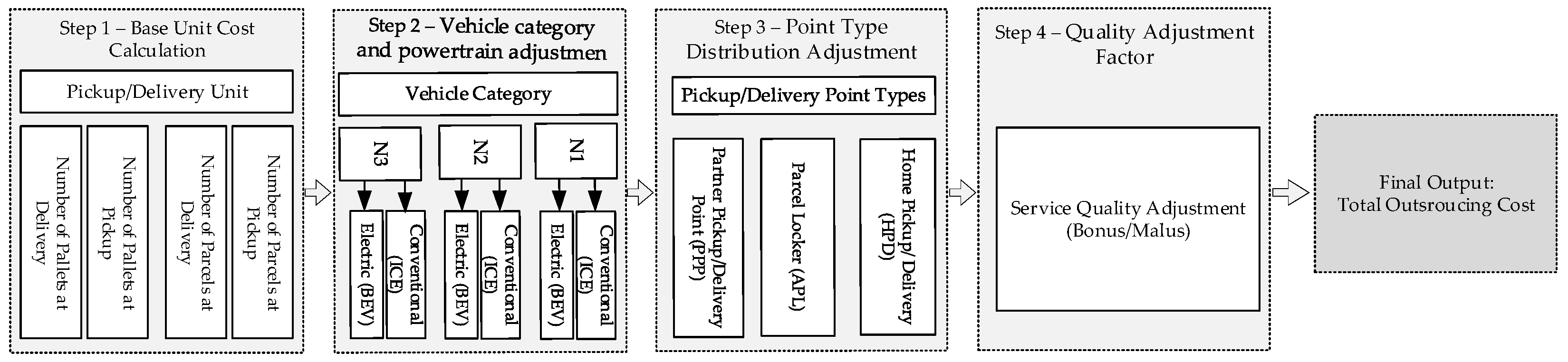
3. Methodology: Proposed Model

This section presents the development of a proposed multidimensional model for calculating outsourcing costs in CEP operations. The model employs a granular approach that considers a combination of factors that influence or may influence the cost in the pickup and delivery stages. These factors include shipment type (parcel or pallet), service phase (pickup or delivery), vehicle category (N1, N2, or N3), vehicle powertrain (conventional or electric), pickup/delivery point type (home address, Parcel Locker, or partner point), and service quality factor. The modeling approach is based on the step-by-step aggregation of base costs, adjusted by corresponding correction factors, ensuring a high level of flexibility and transparency in the cost calculation. The model is suitable for application in real-world CEP operations and can be easily adapted to the internal structure and cost profiles of individual operators.

3.1. Problem Definition

CEP operators face significant challenges in calculating outsourcing costs in the pickup and delivery stages. Existing models typically rely on simplified metrics such as the number of stops, total mileage, or fixed rates per shipment. However, such approaches fail to account for operational elements that substantially affect execution and associated costs. These challenges become even more pronounced when different types of pickup and delivery points, as well as various powertrain types (ICE or BEV), are introduced into the process. The aim of this paper is to propose a model that enables CEP operators to perform granular, transparent, and flexible outsourcing cost calculations aligned with the complexity of daily operations.

This paper is based on the hypothesis that a multidimensional cost allocation model, which systematically incorporates both operational and service-level variables, can provide more accurate and fairer compensation for outsourcing. The model combines technical factors (vehicle category and powertrain type) and operational factors (shipment type, delivery point type, service phase) into a unified structure. Although the model does not formulate an optimization problem in the classical sense (with an objective function and constraints), it enables cost decomposition by service component, thereby supporting informed decision making and contractual fairness.

The model starts from a base cost (unit price per shipment type and service phase) and introduces correction coefficients derived from internal operational data (e.g., TCO, workload at delivery points, SLA compliance). While the Total Cost of Ownership (TCO) requires complex internal estimation processes, its use here is not prescriptive but illustrative, allowing each operator to input their own empirically derived or standardized coefficients.

Ultimately, the model is intended to serve as a transparent analytical tool that bridges the gap between cost awareness and actual outsourcing practice, enabling both principals and contractors to align payments with service complexity.

3.2. Model Notation

This section presents all symbols, sets, indices, and input parameters used in the proposed multidimensional cost allocation model, as shown in

Table 3. Sets and index.

Symbol	Description	Typical Elements
$r$	Route/operation	$r=1,\dots ,n; n\in N\setminus \left\{0\right\}$
$s$	Stage of service	PCK(Pick-up), DEL (Delivery), $s\in \left(PCK,DEL\right)$
$u$	Unit type	PAR (Parcel), PAL (Pallet), $u\in \left(PAR,PAL\right)$
$i$	Vehicle category	$i\in \left(N1,N2, N3\right),$ N1 ≤ 3.5 t, N2 > 3.5 ≤ 12 t, N3 > 12 t
$p$	Powertrain	$\mathrm{ICE}, \mathrm{BEV}, p\in \left(ICE, BEV\right)$
$j$	Pickup/Delivery point	$\mathrm{HPD}, \mathrm{PL}, \mathrm{PPP} (j\in \left(HPD,PL, PPP\right)$
$t$	Observation period	$t=1,\dots ,n; n\in N\setminus \left\{0\right\}$
$\left(u,s\right)$	Combination of unit type and service stage	$\left(PAR,PCK\right),\left(PAL,DEl\right), \mathrm{e}\mathrm{t}\mathrm{c}.$

and

Table 4. Input parameters of the multidimensional model.

Parameter	Description
$N_{s,u,r}$	Number of units u, in phase s, on route r
$N_{r,t}^{u,s,j}$	Number of units of type u, in phase s, at point type j, route r, time t
${\delta }_{u,s}$	$\mathrm{Base} \mathrm{price} \mathrm{per} \mathrm{unit} \mathrm{of} \mathrm{type} u$$\mathrm{in} \mathrm{stage} s$ (e.g., EUR per parcel pickup)
$K_{i,p,r}$	$\mathrm{Cos}\mathrm{t} \mathrm{coefficient} \mathrm{for} \mathrm{vehicle} \mathrm{category} i$$\mathrm{and} \mathrm{powertrain} p$$\mathrm{on} \mathrm{route} r$, estimated via internal TCO or equivalent accounting models
$K_{i,p}^{u,s}$	Cost correction coefficient for vehicle category i, powertrain p, unit type u, and service stage s; expressed as a ratio to the reference configuration (e.g., N1/ICE)
${\alpha }_j^{u,s}$	$\mathrm{Adjustment} \mathrm{factor} \mathrm{for} \mathrm{point} \mathrm{type} j$$\mathrm{and} \mathrm{combination} (u,s)$; values may be derived from operational workload data or route-specific effort levels
$Q_f^{u,s}$	Quality adjustment factor for unit type u and service phase s, reflecting SLA compliance (bonus/malus)
${OC}_{r,t,i,p}^{(u,s)}$	Total adjusted cost per route, unit type, phase, vehicle type, and point

. The model is designed to support flexible cost decomposition based on real-world CEP operations. It combines operational (e.g., shipment type and service phase) and technical (e.g., vehicle category and powertrain) dimensions into a coherent structure. Each parameter is formulated in a way that supports disaggregation, without forcing reduction to a common denominator—thus preserving the multidimensional nature of the problem.

The stepwise structure of the proposed multidimensional model is visualized in Figure 1. The diagram illustrates how the outsourcing cost is calculated through a sequence of four distinct steps.

Note: While the model begins with a lump-sum base cost (e.g., EUR/parcel), it avoids unjustified aggregation by applying empirically justified corrections across each dimension. The use of TCO is not prescriptive, but rather illustrative—operators may substitute their own reliable internal cost coefficients or benchmarking data.

3.3. Mathematical Formulation

The model does not formulate a classical optimization problem with an objective function and constraints. Instead, it follows a deterministic cost decomposition approach, where the total outsourcing cost is computed by summing adjusted cost components derived from operational parameters. The goal is not to minimize or maximize a function, but to provide a transparent and flexible method for cost attribution in line with operational realities. This makes the model especially suitable for contractual settings where fairness, explainability, and adaptability are critical.

The proposed multidimensional model is designed to reflect the real-world complexity of CEP outsourcing through systematic cost aggregation and adjustment. It starts from a base unit cost, defined by shipment type and service phase, and applies a series of correction coefficients that account for vehicle configuration, point type, and service quality. Each component is structured to support disaggregated analysis, enabling operators to identify and manage the cost implications of individual operational factors.

3.3.1. Base Unit Cost Calculation

CEP company N, operating in geographic area A on route r during the observed period t, performs the pickup of a certain number of parcels $N_{PAR, PCK,r}$ and pallets $N_{PAL, PCK,r}$, and delivers a corresponding number of parcels $N_{PAR, DEL,r}$ and pallets $N_{PAL, DEL, r}$. For each combination of transport unit type $u\in \left(PAR,PAL\right)$ and service stage $s\in \left(PCK,DEL\right)$, a base unit price can be defined as follows:

• ${\delta }_{PAR,PCK}$ and ${\delta }_{PAR,DEL}$ for parcels;
• ${\delta }_{PAL,PCK}$ and ${\delta }_{PAL,DEL}$ for pallets.

The base unit prices reflect the standard contractual compensation agreed with subcontractors, prior to any operational adjustment. The total base cost for route r and period t consists of four components and is calculated solely based on the number of parcels and pallets in the pickup and delivery phases, using the base price per unit (parcel/pallet) without any correction factors. It is calculated as follows:

$$\begin{gathered} C_{r,t}^{base}=C_{r,t}^{PAR,PCK}+C_{r,t}^{PAR,DEL}+C_{r,t}^{PAL,PCK}+C_{r,t}^{PAL,DEL} \\ \hspace{1em}\hspace{1em}\hspace{1em}\hspace{1em}\hspace{1em}\hspace{1em}\hspace{1em}\hspace{1em}\hspace{1em}\hspace{1em}\hspace{1em}\hspace{1em}=\sum _{t=1}^n{N}_{PAR, PCK,r}·{\delta }_{PAR,PCK}+\sum _{t=1}^n{N}_{PAR, DEL,r}·{\delta }_{PAR,DEL} \\ \hspace{1em}\hspace{1em}\hspace{1em}\hspace{1em}\hspace{1em}\hspace{1em}\hspace{1em}\hspace{1em}\hspace{1em}\hspace{1em}\hspace{1em}\hspace{1em}+\sum _{t=1}^n{N}_{PAL, PCK,r}·{\delta }_{PAL,PCK}+\sum _{t=1}^n{N}_{PAL, DEL,r}·{\delta }_{PAL,DEL} \end{gathered}$$

(1)

From Equation (1), the following components can be identified as follows:

$C_{r,t}^{PAR,PCK}$—the base cost per parcel in the pickup phase on route r during period t;

$C_{r,t}^{PAR,DEL}$—the base cost per parcel in the delivery phase on route r during period t;

$C_{r,t}^{PAL,PCK}$—the base cost per pallet in the pickup phase on route r during period t;

$C_{r,t}^{PAL,DEL}$—the base cost per pallet in the delivery phase on route r during period t.

This decomposition ensures a modular cost structure that distinguishes between unit type and service phase, enabling subsequent adjustments aligned with real-world operational complexity.

3.3.2. Vehicle Category and Powertrain Adjustments

Vehicle categories refer to classifications based on payload capacity [24]:

• N1 ≤ 3.5 tons;
• N2 > 3.5 ≤ 12 tons;
• N3 > 12 tons.

Therefore, it is first necessary to define the vehicle categories and assign corresponding cost indicators. According to paper [24], reference cost coefficients exist for conventional (ICE) vehicles, which incorporate standard expenses such as fuel, maintenance, depreciation, and other operational costs typically used in contractual pricing. However, in the context of current green delivery trends, these coefficients must be expanded to recognize the powertrain type (ICE or BEV). This enables the model to reflect technological diversity within fleets and to support sustainability objectives via cost-sensitive adjustments. This step does not serve as a constraint or decision variable in an optimization sense. Instead, it deterministically adjusts the base cost using predefined ratios derived from internal company data.

To ensure that the model remains both flexible and grounded in operator-specific data, this phase introduces the cost correction coefficient $K_{i,p}^{u,s}$. This coefficient reflects the relative operational cost of a given combination of vehicle category i and powertrain type p, compared to a predefined reference configuration.

We define

$$K_{i,p}^{u,s}={\displaystyle \frac{{TotalCosts}_{i,p}^{(u,s)}}{{TotalCosts}_{ref}^{(u,s)}}}$$

(2)

where

${TotalCosts}_{i,p}^{(u,s)}$—internally estimated per unit of service stage s on unit type u, using vehicle category i and powertrain p, internally calculated by the company (e.g., Total Cost of Ownership (TCO) or equivalent accounting methods)

${TotalCosts}_{ref}^{(u,s)}$—cost of the reference configuration used as baseline (e.g., N1/ICE) (e.g., N1/ICE).

Importantly, the use of TCO is not prescriptive in this model. While TCO provides a structured methodology for estimating long-term ownership costs (fuel, energy, maintenance, depreciation, and insurance), the model allows operators to apply either empirically derived or benchmarked cost coefficients, depending on their internal accounting capabilities. This ensures that the model remains adaptable to different organizational contexts.

Each of the base costs $C_{r,t}^{u,s}$ from the previous stage (1) is multiplied by its corresponding correction factor $K_{i,p}^{u,s}$:

$$C_{r,t,vehicle}^{PAR,PCK}=C_{r,t}^{PAR,PCK}·K_{i,p}^{PAR,PCK}$$

(3)

$$C_{r,t,vehicle}^{PAR,DEL}=C_{r,t}^{PAR,DEL}·K_{i,p}^{PAR,DEL}$$

(4)

$$C_{r,t,vehicle}^{PAL,PCK}=C_{r,t}^{PAL,PCK}·K_{i,p}^{PAL,PCK}$$

(5)

$$C_{r,t,vehicle}^{PAL,DEL}=C_{r,t}^{PAL,DEL}·K_{i,p}^{PAL,DEL}$$

(6)

where

Vehicle—indicates that the value has been adjusted based on the vehicle category and powertrain type.

$C_{r,t,vehicle}^{PAR,PCK}$—Cost per parcel in the pickup phase on route r, in period t, after adjustment by vehicle category i and powertrain p.

$C_{r,t,vehicle}^{PAR,DEL}$—Cost per parcel in the delivery phase on route r, in period t, after adjustment by vehicle category i and powertrain p.

$C_{r,t,vehicle}^{PAL,PCK}$—Cost per pallet in the pickup phase on route r, in period t, after adjustment by vehicle category i and powertrain p.

$C_{r,t,vehicle}^{PAL,DEL}$—Cost per pallet in the delivery phase on route r, in period t, after adjustment by vehicle category i and powertrain p.

$K_{i,p}^{PAR,PCK}$—Cost correction coefficient for parcels in the pickup phase, when the service is performed using a vehicle of category i and powertrain p.

$K_{i,p}^{PAR,DEL}$—Cost correction coefficient for parcels in the delivery phase, when the service is performed using a vehicle of category i and powertrain p.

$K_{i,p}^{PAL,PCK}$—Cost correction coefficient for pallets in the pickup phase, when the service is performed using a vehicle of category i and powertrain p.

$K_{i,p}^{PAL,DEL}$—Cost correction coefficient for pallets in the delivery phase, when the service is performed using a vehicle of category i and powertrain p.

This modular adjustment structure avoids aggregation across dimensions and preserves the transparency needed for accurate outsourcing cost attribution. Additionally, operators can update correction factors periodically in response to changes in energy prices, vehicle efficiency, or internal cost structures.

Based on the individual costs per service phase and unit type as defined in Equations (3)–(6), the total cost for route r in period t, adjusted for vehicle category and powertrain, is then obtained by summing the adjusted components:

$$C_{r,t}^{vehicle}=C_{r,t,vehicle}^{PAR,PCK}+C_{r,t,vehicle}^{PAR,DEL}+C_{r,t,vehicle}^{PAL,PCK}+C_{r,t,vehicle}^{PAL,DEL}$$

(7)

where

$C_{r,t}^{vehicle}$—Cost adjusted according to vehicle category i and powertrain type p.

3.3.3. Point Type Distribution Adjustment

After the costs in the previous phase have been adjusted according to the vehicle category i and powertrain type p, the model further introduces corrections related to the type of location (point) where pickup or delivery is performed. The cost is thereby differentiated according to the point type j, which enables more detailed tracking and management of operational expenses. These adjustments are deterministic and based on empirically observed effort and workload. They are not derived from a solved optimization but are instead applied as fixed modifiers. The possible types of points are denoted as $j\in \left(HPD,PL, PPP\right)$, where

• HPD—Home Pickup/Delivery;
• PL—Parcel Locker Pickup/Delivery;
• PPP—Partner Pickup Point (e.g., at retail stores or service stations).

Each of these point types carries a different level of operational effort and cost, depending on the following:

• the need for physical delivery (HPD);
• the level of automation and accessibility (PL);
• the involvement of a third party (PPP).

These differences are well-documented in the literature and observed in practice (e.g., lower labor intensity for PLs, shared handling effort in PPPs, and higher travel time for HPD) [31,32]. Therefore, the model adopts a flexible approach to reflect these variances. Since the cost structure can vary significantly between companies, the model does not prescribe fixed weight coefficients. Instead, it allows for flexible input of values ${\alpha }_j$ for each point type $j\in \left(HPD,PL, PPP\right)$, which are to be determined by the company based on its own operational analyses.

These values may be derived from empirical data, time-and-motion studies, or internal routing simulations. For example, a company may assign ${\alpha }_{HPD}=1.00$ as the baseline and calibrate ${\alpha }_{PL}$ or ${\alpha }_{PPP}$ based on observed reductions in dwell time or fuel consumption. This ensures that coefficients reflect actual performance differences and are not arbitrarily selected.

It is important to note that Parcel Lockers (PLs) and Partner Pickup Points (PPPs) are used exclusively for parcels (PARs), whereas pallets (PALs) are delivered only to home or business addresses. Therefore, in modeling the cost distribution by point type, only the number of parcels by point type is taken into account.

For parcels (PARs), an additional correction factor ${\alpha }_j$ may be applied according to the distribution of pickups/deliveries by point type j, and the cost is calculated as follows:

$$C_{r,t,i,p}^{u,s,j}=N_{r,t}^{u,s,j}·{\delta }_{u,s}·K_{i,p}^{u,s}·{\alpha }_j^{u,s}$$

(8)

where

$N_{r,t}^{u,s,j}$—The number of units of type u, in service stage $s\in \left(PCK,DEL\right)$, at point type $j\in \left(HPD,PL, PPP\right)$, on route r during period t;

${\delta }_{u,s}$—The base unit price for shipment type u and service stage s;

$K_{i,p}^{u,s}$—The correction coefficient based on vehicle category i and powertrain type p for the given combination;

${\alpha }_j^{u,s}$—adjustment factor for point type j, for the given service stage $s\in \left(PCK,DEL\right)$, for points of type $j\in \left(HPD,PL, PPP\right)$.

The cost is now broken down by service stage. The disaggregated cost for parcel pickups by point type is calculated using the following formulas:

$$C_{r,t,i,p}^{PAR,PCK,HPD}=N_{r,t}^{PAR,PCK,HPD}·{\delta }_{PAR,PCK}·K_{i,p}^{PAR,PCK}·{\alpha }_{HPD}^{PAR,PCK}$$

(9)

$$C_{r,t,i,p}^{PAR,PCK,PL}=N_{r,t}^{PAR,PCK,PL}·{\delta }_{PAR,PCK}·K_{i,p}^{PAR,PCK}·{\alpha }_{PL}^{PAR,PCK}$$

(10)

$$C_{r,t,i,p}^{PAR,PCK,PPP}=N_{r,t}^{PAR,PCK,PPP}·{\delta }_{PAR,PCK}·K_{i,p}^{PAR,PCK}·{\alpha }_{PPP}^{PAR,PCK}$$

(11)

where

$C_{r,t,i,p}^{PAR,PCK,HD}$—represents the cost of parcel (PAR) pickup at a home address (HD), executed on route r, during period t, using a vehicle of category $i\in \left(N1,N2, N3\right)$ with powertrain $p\in \left(ICE, BEV\right)$, applying the corresponding vehicle and location adjustment factors.

$C_{r,t,i,p}^{PAR,PCK,PL}$—represents the cost of parcel (PAR) pickup at a Parcel Locker (PL), executed on route r, during period t, using a vehicle of category $i\in \left(N1,N2, N3\right)$ with powertrain $p\in \left(ICE, BEV\right)$, applying the corresponding vehicle and location adjustment factors.

$C_{r,t,i,p}^{PAR,PCK,PPP}$—represents the cost of parcel (PAR) pickup at a Partner Pickup Point (PPP), executed on route r, during period t, using a vehicle of category $i\in \left(N1,N2, N3\right)$ with powertrain $p\in \left(ICE, BEV\right)$, applying the corresponding vehicle and location adjustment factors.

The disaggregated cost for parcel deliveries by point type is calculated using the following formulas:

$$C_{r,t,i,p}^{PAR,DEL,HPD}=N_{r,t}^{PAR,DEL,HPD}·{\delta }_{PAR,DEL}·K_{i,p}^{PAR,DEL}·{\alpha }_{HPD}^{PAR,DEL}$$

(12)

$$C_{r,t,i,p}^{PAR,DEL,PL}=N_{r,t}^{PAR,DEL,PL}·{\delta }_{PAR,DEL}·K_{i,p}^{PAR,DEL}·{\alpha }_{PL}^{PAR,DEL}$$

(13)

$$C_{r,t,i,p}^{PAR,DEL,PPP}=N_{r,t}^{PAR,DEL,PPP}·{\delta }_{PAR,DEL}·K_{i,p}^{PAR,DEL}·{\alpha }_{PPP}^{PAR,DEL}$$

(14)

where

$C_{r,t,i,p}^{PAR,DEL,HD}$ represents the cost of parcel (PAR) delivery to a home address (HD), executed on route r, during period t, using a vehicle of category $i\in \left(N1,N2, N3\right)$ with powertrain $p\in \left(ICE, BEV\right)$, applying the corresponding vehicle and location adjustment factors.

$C_{r,t,i,p}^{PAR,DEL,PL}$ represents the cost of parcel (PAR) delivery to a Parcel Locker (PL), executed on route r, during period t, using a vehicle of category $i\in \left(N1,N2, N3\right)$ with powertrain $p\in \left(ICE, BEV\right)$, applying the corresponding vehicle and location adjustment factors.

$C_{r,t,i,p}^{PAR,DEL,PPP}$ represents the cost of parcel (PAR) delivery to a Partner Pickup Point (PPP), executed on route r, during period t, using a vehicle of category $i\in \left(N1,N2, N3\right)$ with powertrain $p\in \left(ICE, BEV\right)$, applying the corresponding vehicle and location adjustment factors.

The total cost for parcel pickup and delivery on route r, in period t, for vehicle i,p is as follows:

$$\begin{gathered} C_{r,t,i,p}^{PAR}=\sum _j\left[N_{r,t}^{PAR,PCK,j}·{\delta }_{PAR,PCK}·K_{i,p}^{PAR,PCK}·{\alpha }_j^{PAR,PCK}+N_{r,t}^{PAR,DEL,j}·{\delta }_{PAR,DEL} \\ ·K_{i,p}^{PAR,DEL}·{\alpha }_j^{PAR,DEL}\right] \end{gathered}$$

(15)

This cost breakdown enables granular tracking of the cost structure across combinations of service phase, point type, vehicle category, and powertrain. Moreover, it allows operators to simulate the impact of changes in delivery structure (e.g., increasing PL usage) on total outsourcing cost—thus promoting strategic redesign of the last-mile network for greater efficiency and sustainability.

3.3.4. Quality Adjustment Factor

After the costs per unit, service stage, point type, vehicle category, and powertrain have been calculated, the final phase of the model applies a service quality adjustment factor. It introduces no optimization logic but rather reflects contractual obligations (bonus/malus) defined in SLA frameworks. The quality modifier adjusts the cost proportionally, with no decision variables involved. This coefficient, denoted as $Q_f^{u,s},$ is defined separately for each combination of transport unit type $u\in \left(PAR,PAL\right)$ and service stage $s\in \left(PCK,DEL\right)$.

In the context of outsourcing contracts, service quality is an important component that often determines the long-term success of cooperation between the principal and the contractor. It reflects not only the technical performance of the subcontractor (e.g., delivery success rate, and damage rate), but also customer satisfaction and compliance with predefined Service Level Agreements (SLAs).

The adjustment is made through a bonus/malus mechanism based on predefined performance indicators (KPIs), within the framework of a Service Level Agreement (SLA) [33,34]. The service quality adjustment factor is calculated using the following formula:

$$Q_f^{u,s}=1+B^{u,s}-M^{u,s}$$

(16)

where

$B^{u,s}$—the relative bonus (%) granted for exceeding KPI thresholds, awarded in case of superior service performance in phase s.

$M^{u,s}$—the relative malus (%) applied for failing to meet quality requirements (e.g., delays, damaged parcels, unsuccessful delivery attempts).

This formulation allows for the transparent operationalization of quality performance in monetary terms, enabling the client to reward good service or penalize underperformance. The values of $B^{u,s}$ and $M^{u,s}$ should be defined contractually based on KPI benchmarks.

The factor $Q_f$ is multiplied by the previously calculated total cost to obtain the final outsourcing cost per route.

The disaggregated cost including the quality factor per service phase can be calculated as follows:

(a)

Cost per parcel in the pickup phase:

$${OC}_{r,t,i,p}^{PAR,PCK}=Q_f^{PAR,PCK}·\sum _j{N}_{r,t}^{PAR,PCK,j}·{\delta }_{PAR,PCK}·K_{i,p}^{PAR,PCK}·{\alpha }_j^{PAR,PCK}$$

(17)

(b)

Cost per parcel in the delivery phase:

$${OC}_{r,t,i,p}^{PAR,DEL}=Q_f^{PAR,DEL}·\sum _j{N}_{r,t}^{PAR,DEL,j}·{\delta }_{PAR,DEL}·K_{i,p}^{PAR,DEL}·{\alpha }_j^{PAR,DEL}$$

(18)

(c)

Cost per pallet in the pickup phase:

$${OC}_{r,t,i,p}^{PAL,PCK}=Q_f^{PAL,PCK}·C_{r,t,vehicle}^{PAL,PCK}$$

(19)

(d)

Cost per pallet in the delivery phase:

$${OC}_{r,t,i,p}^{PAL,DEL}=Q_f^{PAL,DEL}·C_{r,t,vehicle}^{PAL,DEL}$$

(20)

Unlike the previous phases of the model, this quality adjustment mechanism introduces a dynamic behavioral incentive. It enables real-time alignment between cost compensation and service excellence, especially in complex and high-volume delivery environments.

3.3.5. Final Calculation of the Total Outsourcing Cost per Route and Vehicle

Following the step-by-step cost decomposition by shipment type, service phase, vehicle configuration, delivery point type, and service quality, the final outsourcing cost for a given route r and period t is calculated by summing all adjusted cost components.

The total cost is calculated as the sum of the individual cost components defined in Formulas (17)–(20), and is given by the following expression:

$${OC}_{r,t,i,p}={OC}_{r,t,i,p}^{PAR,PCK}+{OC}_{r,t,i,p}^{PAR,DEL}+{OC}_{r,t,i,p}^{PAL,PCK}+{OC}_{r,t,i,p}^{PAL,DEL}$$

(21)

where

• ${OC}_{r,t,i,p}$—represents the final outsourcing compensation to be paid to the subcontractor for executing deliveries on route r, in period t, using a vehicle of category i and powertrain p.
• Each term on the right-hand side corresponds to the total cost component per shipment type and service phase, as adjusted by the vehicle, point type, and service quality.

This formulation serves multiple stakeholders:

• For CEP operators (principals), it supports fair pricing strategies and cost optimization.
• For subcontractors, it ensures compensation is aligned with service complexity and performance quality.

Unlike lump-sum pricing models that obscure internal variability, this model enables transparent, data-driven allocation of costs to actual operational dimensions. In doing so, it supports performance-based contracting, cost control, and potential incentive design for both conventional and sustainable delivery modes.

3.4. Algorithmic Implementation

To facilitate understanding and practical application of the proposed multidimensional model, the following pseudocode outlines the complete step-by-step logic used to calculate the outsourcing cost per route, observation period, vehicle category, and powertrain type. This algorithmic representation directly translates the mathematical formulations presented in Section 3.3 into an executable procedure, making the model operationally transparent and reproducible.

The model does not use an optimization algorithm in the classical sense (with an objective function and constraints), but instead follows a deterministic cost decomposition process that reflects the multidimensional structure of modern CEP outsourcing. It is designed to support granular and fair cost attribution based on shipment type, service phase, vehicle configuration, delivery point type, and service quality. It does not rely on stochastic inputs, heuristic tuning, or machine learning procedures. The full step-by-step implementation logic is presented in Algorithm 1.

Algorithm 1 Practical application of the proposed multidimensional model

Input:   R ← set of routes ($r=1,\dots ,n; n\in N\setminus \left\{0\right\}$)   T ← observation periods   I ← vehicle categories (N1, N2, N3)   P ← powertrain types (ICE, BEV)   U ← unit types (PAR, PAL)   S ← service stages (PCK, DEL)   J ← point types (HPD, PL, PPP) Parameters:   $N_{r,t}^{u,s,j}$ ← number of units by route, period, unit type, service stage, and point type   ${\delta }_{u,s}$ ← base price per unit type and service stage   $K_{i,p}^{u,s}$← vehicle-powertrain cost correction coefficient   ${\alpha }_j^{u,s}$ ← point-based cost adjustment coefficient   $Q_f^{u,s}$ ← service quality adjustment factor (bonus/malus)

Output:   ${OC}_{r,t,i,p}$ ← total outsourcing cost per route, period, vehicle, powertrain

Begin: 1. For each $r$ ∈ R: 2.  For each $t$ ∈ T: 3.   For each $i$ ∈ I: 4.    For each $p$ ∈ P: 5.     Set ${OC}_{r,t,i,p}$ ← 0 6.      For each $u$ ∈ U: 7.       For each $s$ ∈ S: 8.        Set base_cost ← 0 9.          For each $j$ ∈ J 10.           If u = PAL and j ≠ HPD continue 11.           Retrieve units ← $N_{r,t}^{u,s,j}$ 12.           Retrieve unit_cost ← ${\delta }_{u,s}$ 13.           Retrieve k_factor ← $K_{i,p}^{u,s}$ 14.           Retrieve alpha ← ${\alpha }_j^{u,s}$ 15.           Retrieve qf ← $Q_f^{u,s}$ 16.           Compute cost ← units×unit_cost×k_factor×alpha×qf 17.           Update base_cost ← base_cost + cost 18.            End for 19.         Update ${OC}_{r,t,i,p}$ ← ${OC}_{r,t,i,p}$ + base_cost 20.       End for 21.       End for 22.    End for 23.    End for 24.  End for 25. End for 26. Return all ${OC}_{r,t,i,p}\forall r,t,i,p$ values

End

This pseudocode makes explicit the internal logic of the multidimensional model, ensuring clarity for both implementation and validation. By structuring the model in this way, the algorithm supports cost decomposition at any desired level of granularity, from aggregate outsourcing totals down to unit-level cost drivers. This allows CEP operators to align pricing models with actual service complexity and performance.

3.5. Case Study

This section aims to assess the applicability of the proposed multidimensional cost allocation model for outsourcing in CEP operations. The analysis is based on a specific delivery route (denoted as $r=1$) located in an urbanized area in the northeastern region of Bosnia and Herzegovina. Route R1 is operated daily by a battery electric delivery vehicle (BEV) of category N1, covering a mix of pickup and delivery points, including home addresses (HPDs), Parcel Lockers (PLs), and Partner Pickup Points (PPPs). Unlike optimization-based models that seek to minimize total cost or delivery time, this model does not formulate an objective function with constraints. Instead, it follows a deterministic cost decomposition approach that reflects the multidimensional nature of real-world delivery operations.

The study spans four consecutive months in 2024 (January–April), for which actual operational and invoiced data are available. Route $r=1$ is part of a broader network managed by a CEP operator in Bosnia and Herzegovina, consisting of 150 vehicles (90% ICE and 10% BEV) and 150 routes, organized through eight regional centers and one central hub. In line with internal operational policies, certain geographic areas are subcontracted through an outsourcing model with predefined fixed prices per collected and delivered transport unit (parcel/pallet).

The contract with the external operator includes a quality control mechanism (SLA—Service Level Agreement) based on key performance indicators (KPIs), with bonuses and penalties defined as follows: a 4% bonus is awarded for delivery success rates above 97%, while a 4% penalty is applied for rates below 94%.

The objectives of this analysis are as follows:

• To apply the proposed multidimensional model to real-world operational data;
• To obtain an accurate allocation of outsourcing costs based on input parameters such as service phase, shipment type, delivery point type, vehicle category, and powertrain;
• To compare the model results with invoice values calculated using fixed pricing;
• To demonstrate the advantages of the multidimensional approach in terms of transparency, accuracy, and decision-making support for both contractors and service providers.

The following section provides a detailed calculation of outsourcing costs using the proposed multidimensional model for the month of January, while summary results for February, March, and April are presented for the purpose of cost comparison and model accuracy evaluation.

3.5.1. Base Unit Cost Calculation

CEP company N, operating in the urbanized area of northeastern Bosnia and Herzegovina on route $r=1$, collected a certain number of parcels $N_{PAR, PCK,1}$ and pallets $N_{PAL, PCK,1}$, and delivered a corresponding number of parcels $N_{PAR, DEL,1}$ and pallets $N_{PAL, DEL, 1}$ during the observed four-month period $t=\mathrm{1,2},\mathrm{3,4}$, as presented in

Table 5. Overview of the number of picked-up and delivered parcels and pallets over four months on route 1.

Parameter	$\mathbf{January} (\mathit{t}=1)$	$\mathbf{February} (\mathit{t}=2)$	$\mathbf{March} (\mathit{t}=3)$	$\mathbf{April} (\mathit{t}=4)$
$N_{PAR, PCK,1}$	230	218	194	166
$N_{PAR, DEL,1}$	1452	1370	1504	1778
$N_{PAL, PCK,1}$	8	5	16	3
$N_{PAL, DEL, 1}$	53	46	52	60

.

For each combination of shipment type $u\in \left(PAR,PAL\right)$ and service phase $s\in \left(PCK,DEL\right)$, a fixed unit price is defined for each parcel in pickup and delivery as ${\delta }_{PAR,PCK}=1.10 EUR$ and ${\delta }_{PAR,DEL}=1.10 EUR$ and for each pallet in pickup and delivery, as ${\delta }_{PAL,PCK}=5.01 EUR$ and ${\delta }_{PAL,DEL}=5.01 EUR$.

The total base cost for route $r=1$ and period $t=1 month=21 working days)$ consists of four components and is based solely on the number of parcels and pallets in the pickup and delivery phases, applying the base unit price (per parcel/pallet) without any adjustments. It is calculated according to Equation (1) as follows:

$$\begin{gathered} C_{\mathrm{1,1}}^{base}=C_{\mathrm{1,1}}^{PAR,PCK}+C_{\mathrm{1,1}}^{PAR,DEL}+C_{\mathrm{1,1}}^{PAL,PCK}+C_{\mathrm{1,1}}^{PAL,DEL} \\ \hspace{1em}\hspace{1em}\hspace{1em}\hspace{1em}\hspace{1em}\hspace{1em}\hspace{1em}\hspace{1em}\hspace{1em}\hspace{1em}\hspace{1em}\hspace{1em}\hspace{1em}=\sum _{t=1}^1{N}_{PAR, PCK,1}·{\delta }_{PAR,PCK}+\sum _{t=1}^1{N}_{PAR, DEL,1}·{\delta }_{PAR,DEL} \\ \hspace{1em}\hspace{1em}\hspace{1em}\hspace{1em}\hspace{1em}\hspace{1em}\hspace{1em}\hspace{1em}\hspace{1em}\hspace{1em}\hspace{1em}\hspace{1em}\hspace{1em}+\sum _{t=1}^1{N}_{PAL, PCK,1}·{\delta }_{PAL,PCK}+\sum _{t=1}^1{N}_{PAL, DEL,1}·{\delta }_{PAL,DEL} \\ \hspace{1em}\hspace{1em}\hspace{1em}\hspace{1em}\hspace{1em}\hspace{1em}\hspace{1em}\hspace{1em}\hspace{1em}\hspace{1em}\hspace{1em}\hspace{1em}=252.8+1596.2+40.1+265.6=2154.67 EUR \end{gathered}$$

(22)

The base costs were calculated as follows:

• For parcels in the pickup phase on route $r=1$ during period $t=1$ the cost is $C_{\mathrm{1,1}}^{PAR,PCK}=252.8 \mathrm{E}\mathrm{U}\mathrm{R}$;
• For parcels in the delivery phase on the same route and period, $C_{\mathrm{1,1}}^{PAR,DEL}=1596.2 \mathrm{E}\mathrm{U}\mathrm{R}$;
• For pallets in the pickup phase, $C_{\mathrm{1,1}}^{PAL,PCK}=40.1 \mathrm{E}\mathrm{U}\mathrm{R}$;
• For pallets in the delivery phase, $C_{\mathrm{1,1}}^{PAL,DEL}=265.6 \mathrm{E}\mathrm{U}\mathrm{R}$.

This approach clearly defines the base cost by service phase and shipment type.

3.5.2. Cost Calculation by Vehicle Category and Powertrain Adjustment

The vehicle used on route $r=1$ is a light-duty van classified as category N1. According to the paper [24], the coefficient assigned to CEP operators for N1 vehicles is 1.0, which includes standard costs such as fuel, maintenance, depreciation, and others. Since route $r=1$ is operated by a BEV, and given that the multidimensional model accounts for this parameter, it is possible to include it in the cost adjustment—unlike the company’s existing outsourcing model, which does not differentiate based on powertrain type.

As explained in Section 3.3.2, the model does not prescribe a specific methodology for cost estimation, such as Total Cost of Ownership (TCO). Instead, operators are encouraged to apply either TCO-based or empirically derived correction coefficients that best reflect their internal accounting logic, operating context, or benchmarking sources.

The company has 15 BEVs in its fleet, and based on multi-month operational data, a cost correction coefficient has been calculated. This coefficient is not assigned arbitrarily, but is based on empirical internal analysis that compares actual operating cost data for ICE and BEVs under equivalent delivery conditions. It is important to note that Bosnia and Herzegovina offers very limited public incentives for electric vehicle purchases; therefore, the correction coefficient is nearly equivalent to that of ICE vehicles in capital expenditure terms. The correction coefficient for this route and vehicle configuration, $K_{N1,BEV}$, was calculated using internal operational cost estimates, aligned with the company’s accounting methodology and long-term cost tracking. These estimates may be derived from TCO models or equivalent financial structures. For the observed company, BEV-related costs are approximately 5% lower on a monthly basis compared to ICE vehicles. Given that the same vehicle performs both parcel and pallet pickups and deliveries, the same coefficient is applied uniformly.

Now that the BEV correction coefficient of 0.95 (5% reduction) is defined, each of the base costs $C_{r,t}^{u,s}$ from the previous phase can be recalculated by multiplying its respective correction factor $K_{i,p}^{u,s}$. Using Equations (3)–(6), we obtain the following:

$$C_{\mathrm{1,1},vehicle}^{PAR,PCK}=C_{\mathrm{1,1}}^{PAR,PCK}·0.95\%=240.16 \mathrm{E}\mathrm{U}\mathrm{R}$$

(23)

$$C_{\mathrm{1,1},vehicle}^{PAR,DEL}=C_{\mathrm{1,1}}^{PAR,DEL}·0.95\%=1516.39 \mathrm{E}\mathrm{U}\mathrm{R}$$

(24)

$$C_{\mathrm{1,1},vehicle}^{PAL,PCK}=C_{\mathrm{1,1}}^{PAL,PCK}·0.95\%=38.09 \mathrm{E}\mathrm{U}\mathrm{R}$$

(25)

$$C_{\mathrm{1,1},vehicle}^{PAL,DEL}=C_{\mathrm{1,1}}^{PAL,DEL}·0.95\%=252.32 \mathrm{E}\mathrm{U}\mathrm{R}$$

(26)

where

Vehicle—emphasizes that the above values have been adjusted according to both the vehicle category (N1) and the powertrain type (BEV), using operator-specific cost coefficients derived from practical data.

Based on the individual costs per phase and type of transport unit, the total cost per route $r=1$, for the period $t=1$, after the vehicle correction (type and category), it is calculated according to Formula (7) as follows:

$$C_{\mathrm{1,1}}^{vehicle}=C_{\mathrm{1,1},vehicle}^{PAR,PCK}+C_{\mathrm{1,1},vehicle}^{PAR,DEL}+C_{\mathrm{1,1},vehicle}^{PAL,PCK}+C_{\mathrm{1,1},vehicle}^{PAL,DEL}=2046.96 EUR$$

(27)

where

$C_{\mathrm{1,1}}^{vehicle}$—the cost on route $r=1$ in period $t=1$, adjusted according to vehicle category $i=N1$ and powertrain type $p=BEV$.

This approach preserves consistency with the model’s modular logic and supports fair, data-driven compensation schemes for outsourcing in CEP operations.

3.5.3. Calculation of Cost Based on Point Type Distribution Adjustment

After the costs in the previous phase have been calculated for route 1 and a period of 1 month, the model further introduces adjustments based on the type of location (point) at which pickup and delivery operations take place. According to the company’s data, the distribution by pickup points is presented in

Table 6. Overview of parcel and pallet distribution at pickup by point type for January 2024.

Distribution of Parcels and Pallets by Point Type at Pickup	January
HPD PACK	98.00%
HPD PAL	100.00%
PL PACK	1.00%
PPP PACK	1.00%
Distribution of Parcels and Pallets by Point Type at Delivery
HPD PACK	82.0%
HPD PAL	100.0%
PL PACK	8.0%
PPP PACK	10.0%

.

These point-specific adjustments are operationally motivated and allow the model to reflect real-world variations in effort and resource intensity depending on whether a delivery is made to a home address (HPD), a Parcel Locker (PL), or a Partner Pickup Point (PPP).

The reason for such a low percentage of pickups and deliveries at PL and PPPs is that the PL was introduced in November 2023, and there is only one within the area of route 1, while the PPP was introduced in June 2023 at gas stations, where there is also only one within the observed route. On the other hand, this represents a completely new method of pickup and delivery for users, and they are still in the process of adapting to these points.

Given that the CEP operator has signed contracts for PL and PPP, they generate certain costs for the company, which should also be reflected in the outsourcing cost. Since the highest cost is associated with HPD deliveries, it can be treated as the reference value, in accordance with the prices already specified in the contract, which are fixed. Furthermore, the delivery cost for PL and PPP on route 1 is lower. This is primarily due to reduced handling time, lower stop duration, and improved delivery density when using centralized drop-off locations. Vehicles that have PL and PPP points on their routes cover less mileage per pickup/delivery unit and achieve higher consolidation efficiency.

These coefficients are not arbitrarily assigned, but are empirically derived from the company’s operational experience and internal routing data collected over time. The baseline coefficient for HPD (Home Parcel Delivery) is set to 1.00, representing the standard reference point. In contrast, the coefficients for PL (Parcel Locker) and PPP (Pick-up and Drop-off Point) are adjusted proportionally based on observed differences in average stop duration and fuel consumption, recorded during a three-month operational monitoring period. Moreover, it was noted that daily driving distances for routes involving PL and PPP points are generally shorter, which additionally contributes to reduced fuel and time-related costs. These factors together reflect the higher operational efficiency of alternative delivery points compared to standard home delivery.

Based on these analyses, the authors applied correction factors for delivery points, which are presented in

Table 7. Assigned coefficients for pickup and delivery by point type.

Pick/Delivery Point	Correction Coefficient for Parcels $\mathit{\alpha }$ in Pickup and Delivery	Explanation
HPD	1.00	Reference point, most expensive due to home delivery.
PL	0.8	Parcel locker—automated, lower pickup and delivery cost [31,32].
PPP	0.9	Partner Pickup Point—lower workload, but involves human factor.

.

It is important to note that the coefficients presented here are specific to this company’s operational context. However, the model is flexible, and any company implementing it can adjust these coefficients based on its own internal data, delivery structure, and efficiency metrics.

Since pallets are picked up/delivered exclusively to the address, no adjustment is applied, i.e., the correction coefficient is 1.00. The cost can now be calculated and broken down into service phases. The disaggregated cost for parcel pickup by point type is calculated according to Formulas (9)–(11):

$$C_{\mathrm{1,1},N1,BEV}^{PAR,PCK,HPD}=N_{\mathrm{1,1}}^{PAR,PCK,HPD}·{\delta }_{PAR,PCK}·K_{N1,BEV}^{PAR,PCK}·{\alpha }_{HPD}^{PAR,PCK}=235.4 EUR$$

(28)

$$C_{\mathrm{1,1},N1,BEV}^{PAR,PCK,PL}=N_{\mathrm{1,1}}^{PAR,PCK,PL}·{\delta }_{PAR,PCK}·K_{N1,BEV}^{PAR,PCK}·{\alpha }_{PL}^{PAR,PCK}=1.92 EUR$$

(29)

$$C_{\mathrm{1,1},N1,BEV}^{PAR,PCK,PPP}=N_{\mathrm{1,1}}^{PAR,PCK,PPP}·{\delta }_{PAR,PCK}·K_{N1,BEV}^{PAR,PCK}·{\alpha }_{PPP}^{PAR,PCK}=2.20 EUR$$

(30)

The disaggregated cost for parcel delivery by point type is calculated according to Formulas (12)–(14):

$$C_{\mathrm{1,1},N1,BEV}^{PAR,DEL,HPD}=N_{\mathrm{1,1}}^{PAR,DEL,HPD}·{\delta }_{PAR,DEL}·K_{N1,BEV}^{PAR,DEL}·{\alpha }_{HPD}^{PAR,DEL}=1243.41 EUR$$

(31)

$$C_{\mathrm{1,1},N1,BEV}^{PAR,DEL,PL}=N_{\mathrm{1,1}}^{PAR,DEL,PL}·{\delta }_{PAR,DEL}·K_{N1,BEV}^{PAR,DEL}·{\alpha }_{PL}^{PAR,DEL}=97.04 EUR$$

(32)

$$C_{\mathrm{1,1},N1,BEV}^{PAR,DEL,PPP}=N_{\mathrm{1,1}}^{PAR,DEL,PPP}·{\delta }_{PAR,DEL}·K_{N1,BEV}^{PAR,DEL}·{\alpha }_{PPP}^{PAR,DEL}=136.47 EUR$$

(33)

The total cost for parcel pickup and delivery on route r = 1, in period t = 1 month, for vehicle N1, BEV is calculated according to Formula (15):

$$\begin{gathered} C_{\mathrm{1,1},N1, BEV}^{PAR}=\sum _j\left[N_{\mathrm{1,1}}^{PAR,PCK,j}·{\delta }_{PAR,PCK}·K_{N1,BEV}^{PAR,PCK}·{\alpha }_j^{PAR,PCK}+N_{\mathrm{1,1}}^{PAR,DEL,j} \\ ·{\delta }_{PAR,DEL}·K_{N1, BEV}^{PAR,DEL}·{\alpha }_j^{PAR,DEL}\right] \\ \hspace{1em}\hspace{1em}\hspace{1em}\hspace{1em}\hspace{1em}\hspace{1em}\hspace{1em}=235.4+1.92+2.20+1243.41+97.04+136.47 \\ =1716.44 EUR\hspace{1em}\hspace{1em}\hspace{1em}\hspace{1em}\hspace{1em} \end{gathered}$$

(34)

This result illustrates how point-specific corrections influence cost structure. Although home deliveries remain dominant, the inclusion of PL and PPPs—despite being underutilized—already contributes to measurable cost reductions. As the adoption of alternative pickup points increases, this component of the model will become increasingly impactful, providing clear incentives for operators to promote non-home delivery channels.

This method of cost calculation enables detailed tracking of the cost structure for each combination of service phase, point type, vehicle category, and powertrain type.

3.5.4. Calculation of the Quality Adjustment Factor

After the costs per unit, service phase, point type, vehicle category, and powertrain have been calculated, the model anticipates the final phase, which applies the quality adjustment factor.

Since the CEP operator defined SLA (Service Level Agreement) thresholds for bonus and malus when signing the pickup and delivery contract, in this case, the subcontractor achieved a rate of 95.6%. This percentage did not meet the criteria for either a bonus or a malus, and therefore, the quality adjustment factor is 1 (in accordance with Formula (16)).

As a result, the calculated costs will remain unadjusted. The disaggregated cost, including the quality factor per service phase, can be calculated according to Formulas (17)–(20):

(a)

Costs of all parcels in pickup for route 1:

$$\begin{gathered} {OC}_{\mathrm{1,1},N1,BEV}^{PAR,PCK}=Q_f^{PAR,PCK}·\sum _j{N}_{\mathrm{1,1}}^{PAR,PCK,j}·{\delta }_{PAR,PCK}·K_{N1,BEV}^{PAR,PCK}·{\alpha }_j^{PAR,PCK} \\ \hspace{1em}\hspace{1em}=1·\left(235.4+1.92+2.20\right)=239.52 EUR \end{gathered}$$

(35)

(b)

Cost per parcel in delivery for route 1:

$$\begin{gathered} {OC}_{\mathrm{1,1},N1,BEV}^{PAR,DEL}=Q_f^{PAR,DEL}·\sum _j{N}_{\mathrm{1,1}}^{PAR,DEL,j}·{\delta }_{PAR,DEL}·K_{N1,BEV}^{PAR,DEL}·{\alpha }_j^{PAR,DEL} \\ \hspace{1em}\hspace{1em}\hspace{1em}\hspace{1em}=1·\left(1243.41+97.04+136.47\right)=1476.92 EUR \end{gathered}$$

(36)

(c)

Cost per pallet in pickup:

$${OC}_{\mathrm{1,1},N1,BEV}^{PAL,PCK}=Q_f^{PAL,PCK}·C_{\mathrm{1,1},vehicle}^{PAL,PCK}=1·38.09=38.09 EUR$$

(37)

(d)

Cost per pallet in delivery:

$${OC}_{\mathrm{1,1},N1,BEV}^{PAL,DEL}=Q_f^{PAL,DEL}·C_{\mathrm{1,1},vehicle}^{PAL,DEL}=1·252.32=252.32 EUR$$

(38)

The final outsourcing cost according to the proposed multidimensional model for route r = 1, over a period of 21 working days (January), represents the sum of all individual costs arising in the phases of parcel and pallet pickup and delivery, with each of these costs previously adjusted in accordance with the type of transport unit, service phase, vehicle category, powertrain type, pickup/delivery location, and the corresponding quality factor. The final cost is calculated according to Formula (21):

$$\begin{gathered} {OC}_{\mathrm{1,1},N1,BEV}={OC}_{\mathrm{1,1},N1,BEV}^{PAR,PCK}+{OC}_{\mathrm{1,1},N1,BEV}^{PAR,DEL}+{OC}_{\mathrm{1,1},N1,BEV}^{PAL,PCK}+{OC}_{\mathrm{1,1},N1,BEV}^{PAL,DEL} \\ \hspace{1em}\hspace{1em}\hspace{1em}\hspace{1em}\hspace{1em}=239.52+1476.92+38.09+252.32=2006.85 EUR \end{gathered}$$

(39)

The total cost according to the model currently used by the CEP operator for January 2024 amounted to EUR 2154.67. When this amount is compared with the cost obtained using the proposed multidimensional model, which totals EUR 2006.85, a nominal difference of EUR 147.82 is observed, representing a saving of 6.86%. It can also be concluded that the proposed model enables a more accurate, fairer, and more realistic distribution of outsourcing costs. This difference reflects the model’s ability to accurately assign costs based on operational characteristics, rather than relying on fixed prices that ignore variation in vehicle types, service phases, or delivery point structures.

Importantly, this saving is not the result of cost optimization in the mathematical sense, but of improved alignment between actual service complexity and compensation logic. The model does not seek to minimize cost but to transparently and fairly allocate it.

The cost calculation iteration based on the proposed multidimensional model was repeated for the remaining months. An overview of the calculated costs obtained from both the currently used model and the proposed model is presented in

Table 8. Overview of the calculated costs obtained from the currently used model and the multidimensional model.

Calculation Model	$\mathbf{January} (\mathit{t}=1)$	$\mathbf{February} (\mathit{t}=2)$	$\mathbf{March} (\mathit{t}=3)$	$\mathbf{April} (\mathit{t}=4)$
Costs according to the multidimensional model (EUR)	2006.85	1862.85	2052.17	2281.12
Costs according to the current model (EUR)	2154.67	2001.23	220.33	2452.70
Difference (EUR)	147.82	138.37	155.16	171.58
Difference (%)	6.86%	6.91%	7.03%	7.00

.

As shown in Table 8, the model consistently produces cost reductions in the range of 6–7% across multiple periods. These results confirm that the model’s structure—by incorporating relevant operational parameters—leads to more precise and fair outsourcing cost allocation. From a managerial perspective, this level of granularity enables informed contracting decisions and can also serve as a foundation for performance-based remuneration mechanisms.

In scenarios where quality-adjusted bonuses or penalties are applied, the model remains fully functional and scalable, allowing for dynamic adjustment of costs in line with SLA performance levels. Moreover, the model’s modularity makes it suitable not only for auditing existing contracts but also for simulating the impact of network changes, such as shifts in delivery point strategy or fleet electrification levels.

4. Discussion and Conclusions

This paper presents the development and empirical validation of a multidimensional cost calculation model for outsourcing in Courier, Express, and Parcel (CEP) operations. The innovation of the proposed model is its ability to systematically integrate operational (shipment type, service phase, and delivery point) and technical (vehicle category and powertrain) dimensions with a contractual quality component (bonus/malus), within a unified and modular cost structure. This level of integration allows for detailed and fair cost decomposition per route, phase, and delivery condition—going beyond the scope of existing models, which typically isolate such factors or apply simplified heuristics. The model is designed for operational deployment: it does not rely on complex algorithms, but on transparent parameterization that can be adapted to different operators, markets, and data availability levels. This makes the methodology both scalable and transferable, enabling its promotion and replication across different CEP environments. The model addresses a notable gap in the literature, as traditional approaches often oversimplify cost structures by relying on basic metrics such as stop count or distance. By integrating multiple operational and technical parameters—shipment type, service phase, vehicle category, powertrain type, delivery point type, and service quality—the model enables a more nuanced and equitable cost allocation mechanism. The case study results demonstrated the practical relevance of the proposed model. Cost savings of 6% to 8% were consistently observed across four consecutive months when compared to flat rate pricing contracts. These savings were not achieved through optimization techniques but emerged from a more accurate mapping of operational characteristics to compensation logic. The ability to differentiate costs based on vehicle configuration, delivery point type, and service phase is an important contributor to this improvement.

These findings resonate with recent studies advocating for flexible and adaptive cost models in last-mile logistics, especially under growing pressure for efficiency and sustainability. Compared to conventional models based solely on distance, number of stops, or flat rate contracts, the proposed approach offers improved cost attribution without increasing complexity. While some advanced models introduce stochastic or machine learning-based methods, they often lack transparency and modularity, making them less suitable for contractual negotiations. The presented model finds a practical balance between analytical clarity and operational realism.

A key strength of the model lies in its granularity and modularity. It enables route- and phase-specific cost tracking and supports integration into wider logistics planning systems and decision–support tools. The model’s structure allows for scalability across different routes and urban zones, and it provides a reliable basis for outsourcing negotiations, particularly for performance-based contracting through Service-Level Agreements (SLAs). In this context, the model’s quality factor serves not only as a bonus/malus tool but also as a mechanism to support incentive alignment and service-level differentiation—aligning cost structures with contractual performance frameworks. Furthermore, the model’s modularity facilitates its gradual adoption in operational environments, allowing companies to start with simplified configurations (e.g., only by vehicle type) and progressively introduce additional layers such as delivery point type or SLA adjustments. This stepwise adaptability increases the model’s practical viability, even in organizations with limited data infrastructure or analytics capacity.

The findings in this paper are consistent with previous literature advocating for operational differentiation in last-mile delivery cost modeling. The stop-based and distance-based models proposed in [24,25] highlight the limitations of uniform pricing schemes, which the current model addresses through multidimensional cost decomposition. Similarly, our results support conclusions from [31,32], which emphasizes the operational advantages of Parcel Lockers and Partner Pickup Points in reducing time and cost per delivery. However, unlike models such as [20], which treat cost drivers independently and lack service-level correction factors, our approach introduces modular adjustments for vehicle type, powertrain, point of delivery, and SLA compliance. This enables the proposed model to more accurately represent the cost dynamics of urban CEP operations while maintaining transparency and contract-level applicability.

The model provides benefits for both contractual parties involved in CEP outsourcing. On the one hand, CEP operators (principals) gain improved cost transparency and the ability to align compensation with operational complexity across routes and service types. On the other hand, subcontractors benefit from a more equitable and modular compensation structure that fairly reflects the effort associated with different delivery conditions. By replacing lump-sum pricing with component-based logic, the model reduces information asymmetry and fosters balanced, performance-based negotiations between stakeholders.

In terms of theoretical contributions, this research extends the body of knowledge on cost modeling in CEP operations by introducing a comprehensive and operationally grounded framework that overcomes limitations of one-dimensional or aggregated models. The model remains consistent with fundamental principles of transport economics by allocating costs based on measurable operational effort, vehicle utilization, and service differentiation. The methodology and structure of the model are aligned with industry trends toward digitalization, decarbonization, and service personalization.

Nonetheless, several limitations must be acknowledged. First, the model was validated using data from a single urban context in Bosnia and Herzegovina, which may limit the generalizability of findings to other geographic or regulatory settings. Second, while the model introduces correction coefficients (K, α, and Qf), their values are dependent on the availability and quality of internal company data. Without proper calibration, model accuracy may be affected. Third, no sensitivity analysis was conducted to evaluate how variations in input parameters impact final cost outcomes. These aspects present opportunities for further refinement. No anomalies or contradictory effects were observed during empirical application; however, future implementations in different environments may surface trade-offs between service level, environmental performance, and operational cost. If Parcel Lockers or Partner Pickup Points exhibit low user adoption or logistical inefficiencies, the anticipated cost benefits may be reduced or even negated. Likewise, in the absence of reliable input data, correction coefficients may fail to capture the actual operational complexity, potentially resulting in biased cost allocation. Incorporating a dynamic feedback mechanism or adaptive learning layer could enhance the model’s responsiveness over time. While the current model is not formulated as an optimization problem with a formal objective function and constraints, future research could explore its integration into hybrid operations research frameworks—combining deterministic cost decomposition with optimization-based route or resource planning.

The model is particularly valuable for CEP operators, logistics planners, and policymakers who seek to improve cost transparency, optimize outsourcing strategies, and align pricing with operational efficiency and sustainability goals. For contracting authorities (principals), the model supports accurate cost planning, enables fair and performance-based supplier compensation, and facilitates comparison across different service configurations. For subcontractors (service providers), the model ensures that compensation reflects actual delivery complexity, fleet structure, and service-level performance—thus reducing the risk of underpayment in high-effort scenarios and promoting accountability. In practical terms, the model offers:

• Operational accuracy through detailed breakdowns by service phase and delivery type;
• Adaptability to different fleet compositions and internal cost structures;
• Compatibility with electric vehicle usage and alternative delivery points;
• A structured approach for integrating cost logic into route planning and contracting tools, enabling principals to transparently evaluate and compare outsourcing offers, while also allowing contractors to justify cost structures based on service complexity and performance parameters.

In contrast to prior studies that focus on optimization of delivery routes or cost minimization through algorithmic methods, the contribution of this paper lies in formalizing a transparent cost decomposition framework based on operational realities. From a theoretical perspective, the model offers a structured methodology for capturing cost heterogeneity across multiple service dimensions that are typically treated separately in existing literature. It bridges the gap between high-level strategic models and micro-level operational decision-making. In practical terms, the model supports real-time cost attribution and fair compensation design, even in environments where optimization algorithms are impractical due to data limitations or contractual constraints. By shifting the focus from optimization to explainability and adaptability, this work contributes a usable and scalable method for CEP cost modeling in outsourced delivery scenarios.

Future research should explore the integration of this model into multi-route and regional network contexts, as well as its use in dynamic contracting environments where pricing and performance evolve over time. It would also be valuable to extend the quality adjustment factor into a fully quantitative SLA-monitoring module that links cost variation to defined KPIs and service benchmarks. Additionally, implementing a sensitivity analysis across different parameter scenarios would help in assessing the robustness of cost estimations.

In conclusion, the proposed multidimensional model offers a robust, scalable, and practically oriented framework for cost allocation in outsourced CEP services. By bridging the gap between operational detail and contractual application, the model promotes both fairness and accountability. Its application not only improves pricing accuracy and operational efficiency but also establishes a transparent and accountable basis for structuring outsourcing relationships—advancing strategic goals such as cost control, service quality, and environmental sustainability in modern CEP networks.

References

1. Ghazal, A.; Narayanan, S.; Adeniran, I.O.; Dörpinghaus, J.; Drees, L. Analysis of Logistics Measures of CEP Service Providers for the Last-Mile Delivery in Small- and Medium-Sized Cities: A Case Study for the Aachen City Region. Eur. Transp. Res. Rev. 2025, 17, 5. [Google Scholar] [CrossRef]
2. Viu-Roig, M.; Alvarez-Palau, E.J. The Impact of E-Commerce-Related Last-Mile Logistics on Cities: A Systematic Literature Review. Sustainability 2020, 12, 6492. [Google Scholar] [CrossRef]
3. Boysen, N.; Fedtke, S.; Schwerdfeger, S. Last-Mile Delivery Concepts: A Survey from an Operational Research Perspective. OR Spectr. 2021, 43, 1–58. [Google Scholar] [CrossRef]
4. Bosona, T. Urban Freight Last Mile Logistics—Challenges and Opportunities to Improve Sustainability: A Literature Review. Sustain. 2020, 12, 8769. [Google Scholar] [CrossRef]
5. Laseinde, O.T.; Mpofu, K. Providing Solution to Last Mile Challenges in Postal Operations. Int. J. Logist. Res. Appl. 2017, 20, 475–490. [Google Scholar] [CrossRef]
6. Ducret, R. Parcel Deliveries and Urban Logistics: Changes and Challenges in the Courier Express and Parcel Sector in Europe—The French Case. Res. Transp. Bus. Manag. 2014, 11, 15–22. [Google Scholar] [CrossRef]
7. Goigi. Retail E-Commerce. 2023. Available online: https://www.goigi.com/frontend/Retail_Ecommerce.pdf (accessed on 8 May 2025).
8. Otto, A.; Boysen, N.; Scholl, A.; Walter, R. Ergonomic Workplace Design in the Fast Pick Area. OR Spectr. 2017, 39, 945–975. [Google Scholar] [CrossRef]
9. Sawik, B. Optimizing Last-Mile Delivery: A Multi-Criteria Approach with Automated Smart Lockers, Capillary Distribution and Crowdshipping. Logistics 2024, 8, 52. [Google Scholar] [CrossRef]
10. Latif, N.A.; Stephen, D.; Abu Mansor, S.; Adruce, S.A.Z. Fostering Economic Sustainability through the Pick-Up and Drop-Off (PUDO) Point Suitability Index: Optimising Last-Mile Delivery Efficiency. J. Sustain. Sci. Manag. 2025, 20, 101–121. [Google Scholar] [CrossRef]
11. Ranjbari, A.; Diehl, C.; Dalla Chiara, G.; Goodchild, A. Do Parcel Lockers Reduce Delivery Times? Evidence from the Field. Transp. Res. Part E Logist. Transp. Rev. 2023, 172, 103070. [Google Scholar] [CrossRef]
12. Mogire, E.; Kilbourn, P.; Luke, R. Electric Vehicles in Last-Mile Delivery: A Bibliometric Review. World Electr. Veh. J. 2025, 16, 52. [Google Scholar] [CrossRef]
13. Oshri, I.; Kotlarsky, J.; Willcocks, L.P. The Handbook of Global Outsourcing and Offshoring; Springer: Cham, Switzerland, 2023. [Google Scholar] [CrossRef]
14. Tsai, C.-A.; Ho, T.-H.; Lin, J.-S.; Tu, C.-C.; Chang, C.-W. Model for Evaluating Outsourcing Logistics Companies in the COVID-19 Pandemic. Logistics 2021, 5, 64. [Google Scholar] [CrossRef]
15. Akhtar, M. Logistics Services Outsourcing Decision Making: A Literature Review and Research Agenda. Int. J. Prod. Manag. Eng. 2023, 11, 73–88. [Google Scholar] [CrossRef]
16. Charles, M.; Ochieng, S.B. Strategic Outsourcing and Firm Performance: A Review of Literature. Int. J. Soc. Sci. Humanit. Res. 2023, 1, 20–29. [Google Scholar] [CrossRef]
17. Zäpfel, G.; Bögl, M. Multi-Period Vehicle Routing and Crew Scheduling with Outsourcing Options. Int. J. Prod. Econ. 2008, 113, 980–996. [Google Scholar] [CrossRef]
18. Ülkü, M.A.; Bookbinder, J.H. Optimal Quoting of Delivery Time by a Third Party Logistics Provider: The Impact of Shipment Consolidation and Temporal Pricing Schemes. Eur. J. Oper. Res. 2012, 221, 110–117. [Google Scholar] [CrossRef]
19. Chaabouni, F.; Dhiaf, M.M. Logistics Outsourcing Relationships: Conceptual Model. In Proceedings of the 2013 International Conference on Advanced Logistics and Transport (ICALT), Sousse, Tunisia, 29–31 May 2013; pp. 458–463. [Google Scholar] [CrossRef]
20. Gevaers, R.; Van de Voorde, E.; Vanelslander, T. Cost Modelling and Simulation of Last-Mile Characteristics in an Innovative B2C Supply Chain Environment with Implications on Urban Areas and Cities. Procedia Soc. Behav. Sci. 2014, 125, 398–411. [Google Scholar] [CrossRef]
21. Ko, S.Y.; Cho, S.W.; Lee, C. Pricing and Collaboration in Last Mile Delivery Services. Sustainability 2018, 10, 4560. [Google Scholar] [CrossRef]
22. Roy, J.; Pamučar, D.; Kar, S. Evaluation and Selection of Third Party Logistics Provider under Sustainability Perspectives: An Interval Valued Fuzzy-Rough Approach. Ann. Oper. Res. 2020, 293, 669–714. [Google Scholar] [CrossRef]
23. Krstić, M.D.; Tadić, S.R.; Brnjac, N.; Zečević, S. Intermodal Terminal Handling Equipment Selection Using a Fuzzy Multi-Criteria Decision-Making Model. Promet–Traffic Transp. 2019, 31, 89–100. [Google Scholar] [CrossRef]
24. Kosovac, A.; Muharemović, E. Pickup and Delivery Costs—A Proposed Outsourcing Model Based on the Number of Stops. J. Appl. Eng. Sci. 2021, 19, 270–274. [Google Scholar] [CrossRef]
25. Kosovac, A.; Muharemović, E.; Trubint, N. A Cost Calculation Model for Outsourcing in Parcel Pick-up and Delivery by Commercial Postal Services Operators. TEM J. 2020, 9, 216–220. [Google Scholar] [CrossRef]
26. Su, E.; Qin, H.; Li, J.; Pan, K. An Exact Algorithm for the Pickup and Delivery Problem with Crowdsourced Bids and Transshipment. Transp. Res. Part B Methodol. 2023, 177, 102831. [Google Scholar] [CrossRef]
27. Alnaggar, A.; Gzara, F.; Bookbinder, J.H. Compensation Guarantees in Crowdsourced Delivery: Impact on Platform and Driver Welfare. Omega 2024, 122, 102965. [Google Scholar] [CrossRef]
28. Schur, R.; Winheller, K. Optimizing Last-Mile Delivery: A Dynamic Compensation Strategy for Occasional Drivers. OR Spectr. 2024. [Google Scholar] [CrossRef]
29. Dong, C.; Huang, Q.; Pan, Y.; Ng, C.T.; Liu, R. Logistics Outsourcing: Effects of Greenwashing and Blockchain Technology. Transp. Res. Part E Logist. Transp. Rev. 2023, 170, 103015. [Google Scholar] [CrossRef]
30. Wang, Z.; Zhu, R.; Ding, J.Y.; Yang, Y.; You, K. Localized Package Shipment with Partial Outsourcing: An Exact Optimization Approach for Chinese Courier Companies. Transp. Res. Part E Logist. Transp. Rev. 2025, 194, 103901. [Google Scholar] [CrossRef]
31. Taniguchi, E.; Thompson, R.G.; Qureshi, A.G. Modelling City Logistics Using Recent Innovative Technologies. Transp. Res. Procedia 2020, 46, 3–12. [Google Scholar] [CrossRef]
32. Seghezzi, A.; Siragusa, C.; Mangiaracina, R. Parcel Lockers vs. Home Delivery: A Model to Compare Last-Mile Delivery Cost in Urban and Rural Areas. Int. J. Phys. Distrib. Logist. Manag. 2022, 52, 213–237. [Google Scholar] [CrossRef]
33. Qi, F.; Zhou, G. An SLA-Based Performance Monitoring Mechanism for 3PL Business Process. J. Residuals Sci. Technol. 2016, 13, 51.1–51.6. [Google Scholar]
34. Selviaridis, K.; Norrman, A. Performance-Based Contracting for Advanced Logistics Services. Int. J. Phys. Distrib. Logist. Manag. 2015, 45, 592–617. [Google Scholar] [CrossRef]
Figure 1. Process flow diagram of the proposed multidimensional model for outsourcing cost calculation in CEP operations.
Logistics 09 00096 g001