Managing Home Healthcare System Using Capacitated Vehicle Routing Problem with Time Windows: A Case Study in Chiang Mai, Thailand

Abstract

Background: The Vehicle Routing Problem with Time Windows (VRPTW) has been extensively researched due to its applicability across various real-world domains, including logistics, healthcare, and distribution systems. With the global elderly population projected to continue increasing, the demand for home healthcare (HHC) services is also on the rise. This work focuses on a specific application within an HHC system, aiming to minimize the total completion time for a fleet of vehicles delivering healthcare services to patients at home. Methods: We propose a mathematical model for the VRPTW, targeting a reduction in both customer and server waiting times on each route and seeking to decrease the total completion time. Our proposed algorithm employs a tabu search to narrow the search space, leveraging a greedy algorithm to establish the tabu list. Results: Our experimental results, based on Solomon’s benchmark datasets, demonstrate that the proposed algorithms achieve optimal solutions, particularly in minimizing total completion time compared to traditional methods, in a case study involving 400 customers where vehicles’ hours are restricted to align with caregivers’ average daily working hours. Conclusions: Our algorithm resulted in a 59% reduction in the number of vehicles required compared to the most recent algorithms, which combine k-mean clustering and local search.

1. Introduction

The VRPTW is a complex combinatorial optimization problem that extends the classic Vehicle Routing Problem (VRP) by incorporating time windows governing the start and end of services to a customer. The goal is to determine the optimal set of routes for a fleet of vehicles to service a given set of customers within a particular set of time windows while minimizing the overall cost, typically measured in terms of total distance or time. The VRPTW has significant practical applications in logistics, transportation, and distribution. For example, the VRPTW in a waste collection problem [1] aims to minimize the number of required trucks and their total route time while trying to satisfy the customers’ time windows. The VRPTW in China’s vegetable and food distribution by Zhang et al. [2] minimizes the total distribution cost. The VRPTW in China’s supermarket food distribution described by Huang et al. [3] minimizes the total distribution cost, including vehicle usage and travel and unpunctuality penalty costs. The VRPTW in a logistic system for bottled-product distribution by Gómez et al. [4] minimizes the travel and waiting times required to service all customers while also minimizing the number of vehicles needed. The VRPTW is applied to healthcare systems in [5], improving the pharmaceutical distribution system by arranging the optimal route for delivering to pharmacies. Moreover, as in [6], it enhances the quality of the HHC services while minimizing travel costs and taking into account the time window limitation of patients and the expertise levels of the team.

Over the past 50 years, the percentage of elderly people over 65 has almost doubled from 5.5% to 10.3% of the world’s total population [7]. The World Health Organization stated in [8] that the over-60 population as a percentage of the global population will nearly double from 12% in 2015 to 22% by 2050. The population aging trend started in high-income countries and then shifted to middle- and low-income countries. In 2023, the over-65 population made up more than 20% of the population of nearly every country in Europe, making these countries super-aged societies according to the United Nations’ definition [9]. Moreover, 6% of the population of these countries is estimated to be over 80 years of age [10]. People who are 80 years old and over tend to have increased needs to access healthcare and medical care. In Asia, Japan and Hong Kong became super-aged societies in 2005 and 2022, respectively. In 2023, over 30% of the Japanese population was over 65 years old, and 10% was over 80 years old; the same figures in Hong Kong were 21% and 5%, respectively [11]. Thailand became an aging society in 2007, when its over-65 population reached 10% of the total population, and became an aged society in 2020, when its over-65 population reached 14% of the total population [11]. The United Nations estimated that, by 2030, Thailand will become a super-aged society with 20% of its population over 65 years of age [12].

The HHC system is crucial for an aging population as it provides services to elderly individuals and other patients whose mobility issues prevent them from traveling to a hospital to receive care. HHC services typically require time windows on home visits as some of the services may be time sensitive. Consequently, the VRPTW has been widely applied to HHC problems. Tailored algorithms have been constructed to solve the model due to its NP-hard nature. In 2013, Liu et al. [13] studied the delivery of drugs and medical devices from healthcare centers to patients’ homes, as well as the pickup of bio-samples from patients to healthcare centers. They proposed heuristics based on tabu search and genetic algorithms, testing their methods on a modified, well-known benchmark instance. In 2016, Haddadene et al. [14] added synchronization and precedence constraints to improve HHC service quality. They proposed a mixed-integer linear programming model and developed a greedy heuristic, local search, and three metaheuristics to solve their model. Experimental results show that solutions for small (18-customer), medium (45-customer), and large (73-customer) instances can be found within an acceptable time by their metaheuristics, and their approach was more general than the previous methods. In 2019, Liu et al. [15] proposed a mathematical model for an HHC system based on route construction and developed a branch-and-price algorithm. They examined the performance of their algorithm via small test instances with 30 customers and five vehicles, medium-size instances with 40 customers and seven vehicles, and large instances with 50 customers and nine vehicles. In 2020, Euchi et al. [16] also studied the VRPTW with synchronized visits. They proposed an ant colony system with a clustering algorithm to improve the quality of HHC in terms of the total time necessary for caregivers to visit all patients by considering case priorities. In 2021, Chaieb and Sassi [17] studied a bi-objective problem that minimizes travel time and distance in the HHC problem. They solved the proposed model using a k-means clustering algorithm and tabu search. To improve HHC services with an environmentally friendly approach, the multi-objective function of Green Home Health Care (GHHC) was studied by Makboul et al. [18]. Their goal was to minimize the total travel distance and CO2 emissions while ensuring a balanced workload for caregivers and meeting patient satisfaction.

Algorithms to solve an NP-hard problem such as the VRPTW can be divided into three major categories: (1) exact algorithms, (2) heuristic algorithms, and (3) hybrid metaheuristics. Exact algorithms can obtain an optimal solution. They are suitable for small-to-medium-sized instances, but struggle with larger problems due to computational complexity. Examples of exact algorithms include branch-and-bound, branch-and-cut, dynamic programming, and column generation. Heuristic algorithms are designed to solve problems more quickly than exact algorithms. Examples of heuristic algorithms include tabu search, genetic algorithms, simulated annealing, and ant colony optimization. To quickly and efficiently attain a nearly optimal solution, many researchers have proposed combining the strengths of various heuristics into hybrid metaheuristics. The following works are related to heuristic algorithms and hybrid metaheuristics for the VRPTW. In 2013, Baños et al. [19] presented a new hybrid metaheuristic algorithm known as a multi-start multi-objective evolutionary algorithm combined with simulated annealing, which can be executed in a sequential or parallel process. In 2014, Hifi and Wu [20] proposed a hybrid metaheuristic algorithm combining ant colony optimization with a large neighborhood search. In 2019, François et al. [21] developed an adaptive large neighborhood search algorithm that started with an initial solution and iteratively improved the best solution by exploring large neighborhoods. The customers were then removed from a part of the solution and a new solution was reconstructed in each iteration. In 2023, Ahmed et al. [22] proposed a modified football game algorithm that generated initial solutions and an efficient mechanism for creating new positions for the players (vehicles), and Saksuriya and Likasiri [23] proposed k-means clustering and local search to minimize completion time. Then in 2024, Bin Yue et al. [24] introduced an improved initialization algorithm that quickly generated initial feasible solutions by focusing on the compatibility index of distance and time windows and proposed a tabu search method.

Benchmark instances are valuable for testing and comparing the performance of constructed algorithms. In 1987, Solomon [25] introduced instances for the VRPTW which later became benchmark instances commonly referred to as Solomon’s benchmark instances. The data sets are randomly generated in three main types including clustered, random, and randomly clustered instances, with the wide and narrow time windows of 100 customers. At present, over 3000 works have used Solomon’s benchmark instances to test their proposed algorithms. To test exact algorithms, some researchers reduced the number of customers in Solomon’s instances to small sizes including 25 and 50 customers. For example, Kallehauge et al. [26] studied exact algorithms such as branch-and-bound and branch-and-cut for solving the VRPTW problem and showed the efficiency of the algorithm via small sizes (25, 50, and 100 customers) of Solomon’s benchmark instances. Bräysy and Gendreau [27] studied the basic features of existing algorithms which are tradition route construction techniques and local search methods and compared their performance using the original Solomon’s instances. Later, the same authors analyzed and compared existing metaheuristics including tabu search, genetic algorithms, and other advanced techniques for solving the VRPTW [28]. Solomon’s instances were also tested by Baños et al. [19], Hifi and Wu [20], François et al. [21], Ahmed et al. [22], Bin Yue et al. [24], etc.

Other well-known instances of the VRPTW include those by Gehring and Homberger [29], introduced to test their hybrid algorithm combining evolutionary and tabu search methods. Gehring and Homberger’s instances were extended from Solomon benchmark to large-sized problems including 200, 400, 800, and 1000 customers for testing the existing method. Zong et al. [30] tested their algorithm using Gehring and Homberger’s instances. They proposed a reinforcement learning method enhanced with a time penalty augmented reward to incorporate time-window constraints during the learning process to minimize the travel distance of the VRPTW and applied it using real-world datasets. In addition, there are other instances related to time windows, such as benchmark instances for pickup and delivery vehicle routing problems with time windows and multiple vehicles (PDPTW) [31], benchmark instances for the periodic VRPTW (PVRPTW), for the multi-depots (MDVRPTW), for vehicle-site dependencies (SDVRPTW) [32], for the vehicle routing problem with time windows on a road network called NEWLET [33], for the simultaneous delivery and pickup problem with time windows (SDPPTW) [34], and for the multi-objective vehicle routing problem with time windows (MOVRPTW) [35].

Common objective functions of the VRPTW are minimization of the total travel distance, total travel time, or the number of utilized vehicles, or combinations of these three objectives or other multi-objectives of the VRPTW. Examples of objective functions tackled are as follows. Works tackled as a single objective are minimizing both travel distance and route imbalances in [19] and minimizing the total travel distance and balancing the length of routes in [36]. Two objectives are considered in the bi-objective to minimize the number of vehicles and the travel distances in [20], and the bi-objective to minimize travel costs and maximize customers’ demand satisfaction in [37]. Some works with multiple objectives are minimizing the total travel distance, minimizing fixed vehicle costs, and maximizing customer satisfaction, which is achieved by the minimization of the penalties for early or late arrivals at customer locations [2], minimizing the number of vehicles, total travel time, total waiting time, and the longest travel time among all routes [35], and minimizing the completion time including the travel time, waiting time, and operating time [23]. The summary of the literature is shown in

Table 1. Summary of existing algorithms, benchmark instances for testing the performance of algorithms, and real-world applications.

VRP on Distribution Problems
Model	Objective	Algorithms	Benchmarks/Size	Applications/Size	Ref.
Roll-in–roll-off VRPTW	Minimize the number of vehicles and their total route time	Large neighborhood search	N/A	Waste collection in US/6-291	[1]
VRPTW	Minimize the number of vehicles and their total route time	Ant colony	Solomon/100	N/A	[4]
VRPTW	Minimize the total travel distance	Scatter search	Solomon/25–100	Company in Tenerife, Spain/N/A	[36]
Multi-objective VRP with flexible time windows	Minimize the total travel cost and total fixed vehicle costs	Ant colony	Solomon/100	Vegetable and food distribution in Beilin district, Xi’an, China/16	[2]
VRPTW	Minimize the total travel cost and maximize the total quality of service	Hybrid genetic algorithm and simulated annealing	GHHC instances/4–75	N/A	[6]
VRP for fresh products distribution considering customer satisfaction	Minimize the total travel cost and total fixed vehicle costs	Large neighborhood search	Solomon/25–50	Fresh food distribution in Beijing/25	[3]
VRPTW	Minimize the total travel distance	Exact algorithm and several heuristics	N/A	Pharmaceutical distribution in Morocco/12	[5]
VRPTW	Minimize the total completion time	Modified k-means and local search	Solomon/100	HHC in Chiang Mai/400	[23]
VRPTW	Minimize the total travel distance	Reinforcement learning	Homberger/1000	Online operation system of Hitachi in Guangzhou/500–700	[30]
VRP on HHC problems
Model	Objective	Algorithms	Benchmarks/Size	Applications/Size	Ref.
VRP with simultaneous delivery and pickup and time windows	Minimize the total travel cost	Genetic algorithm and tabu search	Solomon and Homberger/100–400	N/A	[13]
VRPTW synchronization and precedence constraints	Minimize the total travel time and the sum of non-preferences	Hybrid greedy and local search	HHC instances/18–73	N/A	[14]
Multiple depot VRP with stochastic travel and service time	Minimize the total travel cost	Branch-and-price algorithm	Instances generated by the authors/30–50	N/A	[15]
VRPTW with synchronization visits	Minimize the total travel cost	Ant colony	Bredström and Rönnqvist’s instances/20–80	N/A	[16]
VRP with simultaneous delivery and pickup and time windows	Minimize the total travel cost	K-means and tabu search	Solomon/25	N/A	[17]
VRP/MILP	Minimize the total travel distance and CO2 emissions/maximize to ensure a fair workload	Genetic algorithm	TSPTW instances/200	N/A	[18]
Works related to time windows
Model	Objective	Algorithms	Benchmarks/Size	Applications/Size	Ref.
VRPTW	Minimize the total travel time or distance	Development of saving algorithm, nearest neighbor algorithm, insertion algorithm, and sweep algorithm	Solomon/100	N/A	[25]
VRPTW	Minimize the number of vehicles and total travel distance	Hybrid evolutionary and tabu search	Solomon and Homberger/100–1000	N/A	[29]
VRPTW	Minimize the total travel time or distance	Route construction and local search	Solomon/100	N/A	[27]
VRPTW	Minimize the total travel time or distance	Tabu search and genetic algorithm	Solomon/100	N/A	[28]
VRPTW	Minimize the number of vehicles and total travel distance	Branch-and-bound and column generation	Solomon/25–100	N/A	[26]
PDPTW	Minimize the number of vehicles and total travel distance	Simulated annealing and large neighborhood search	PDPTW instances/100–600	N/A	[31]
SDPPTW	Minimize the total travel cost	Genetic algorithm	SDPPTW instances (revised from Solomon)/25–100	N/A	[34]
MOVRPTW	Minimize the total travel distance and distance imbalance among routes	Simulated annealing	Solomon/100	N/A	[19]
VRPTW, PVRPTW, MDVRPTW, SDVRPTW	Minimize the total travel distance	Hybrid genetic search and adaptive diversity control algorithm	Solomon, Homberger, PVRPTW, MDVRPTW, and SDVRPTW instances/100–1000	N/A	[32]
VRPTW	Minimize the number of vehicles and total travel distance	Hybrid ant colony and large neighborhood search	Solomon and Homberger/100–200	N/A	[20]
Electric VRPTW	Minimize the total travel distance	Hybrid variable neighborhood search and tabu search	Extended Solomon/100	N/A	[38]
Multi-trip VRPTW	Minimize the total duration and travel time	Adaptive large neighborhood search	Solomon/100	N/A	[21]
MOVRPTW	Minimize the total travel cost and maximize customers’ demand satisfaction	Non-dominated sorting genetic algorithm	Solomon/25–100	N/A	[37]
Time-dependent VRPTW	Minimize the total travel time	Tabu search heuristic	NEWLET/50–200	N/A	[33]
MOVRPTW	Minimize the number of vehicles, total travel distance, total waiting time, and total delay time	Non-dominated sorting genetic algorithm	MOVRPTW instances/50–250	N/A	[35]
Electric VRPTW	Minimize the total travel distance	Large neighborhood search	Extended Solomon/100	N/A	[39]
VRPTW	Minimize the total travel distance	Modified football game	Solomon/100	N/A	[22]
Electric VRPTW	Minimize the total travel distance and total recharging cost	Local search and dynamic programming	Solomon and Extended Solomon/100	N/A	[40]
VRPTW	Minimize the total travel distance	Tabu search and variable neighborhood search	Solomon/25–100	N/A	[24]

.

We are interested in HHC problems where caregivers are required to serve customers within an 8 h workday. To find the solutions to satisfy this condition, we will minimize the completion time, including total travel time, waiting time, and operating time of each caregiver. The VRPTW is studied to tackle the HHC problem in which each vehicle is identified as a caregiver. A mathematical model has been developed to minimize the total completion time. Note that vehicles with fewer waiting hours are prone to finish sooner than those with longer waiting times. Minimizing the total waiting time should consequently minimize the total completion time. Our proposed algorithm aims to achieve this by utilizing a greedy search approach to reduce completion time, combined with a tabu search algorithm to limit the search space for solutions. The first phase is to find the initial feasible solution and the second phase is to improve the solution using a tabu list. Our tabu search techniques iteratively improve an initial solution by using memory structures to avoid cycles and help improve the search process. Since the objective function of our proposed model differs from those of previous studies, we tested small instances from Solomon’s dataset with 25 customers to find optimal solutions. The efficiency of the proposed algorithm was evaluated by comparing the obtained solutions to the optimal solutions in these small instances. To illustrate the efficiency of the proposed algorithm in large-size problems, we also find the solutions of Solomon’s instances with 100 customers for this particular objective function. Then, to amplify the utilization of our proposed algorithm, we tackle an HHC case study in Chiang Mai, a popular retirement destination and home to Thailand’s third-largest over-65 population.

The remainder of this paper is organized as follows: Section 2 describes the mathematical model, which is adapted from the VRPTW to suit our specific requirements. Section 3 presents our proposed algorithm, consisting of two phases: solution initialization and solution improvement. Section 4 details our computational experiments, which examine the performance of the proposed algorithm on both small and large instances. Section 5 applies the algorithm to a case study on the HHC in Chiang Mai province involving 400 customers [23]. Conclusions and discussions are provided in the last section.

2. Mathematical Formulation

A VRPTW considered in this work consists of a single center responsible for delivering services to customers at their homes during a typical workday. Each service provider, e.g., a caregiver, has limited working hours. Customers will only be served by vehicles operating within their specified availability windows. Each vehicle will start and end its route at the service center. The total demand from all customers will not exceed the vehicle’s capacity. The objective of the VRPTW is to minimize the total completion time, which includes travel time consisting of travel times from the service center to customers and return time to center, waiting time, and service time for each vehicle while adhering to the caregiver’s working time constraints.

The VRPTW problem can be written in the form of a network consisting of a set $N=I\cup \left\{0\right\}$ being nodes in the network with $I=\left\{1,\dots ,n\right\}$ being customer nodes, and 0 being the center node. Edges linked between 2 nodes in the network represent the road links between two nodes in the real system. Every vehicle will start and end at the center. Each customer must be served within their available time, called the time window. The finish time of the last customer together with the return time to the center of each vehicle must not exceed the maximum working hours of the caregiver. The service and travel times at customer locations are provided. The associated mathematical formulation is defined as a VRPTW where the objective is to minimize the total completion time (VRPTW-CT). The indices, parameters, and variables related to the model are presented below.

• Indices:
  0 The starting node and the end node of all vehicles, here called the center
  $i,j$ The customer $i,j\in \left\{1,2,\dots ,n\right\}$
  $k$ The vehicle $k\in \left\{1,2,\dots ,m\right\}$

• Parameters:
  $c_{ij}$ The travel time from customer $i$ to customer $j$
  $r_i$ The available time for customer $i$
  $e_i$ The end time for customer $i$
  $p_i$ The service time for customer $i$
  $d_i$ The customer demand $i$
  $Q$ The capacity of all vehicles
  $M$ A sufficiently large number
  $T$The maximum working hours of the caregiver.

• Variables:
  $x_{0j}^k$ equal to 1 if the vehicle $k$ starts from the center to customer $j$; otherwise, 0
  $x_{ij}^k$ equal to 1 if vehicle $k$ travels from customer $i$ to customer $j$; otherwise, 0
  $x_{j0}^k$ equal to 1 if customer $j$ is the last customer visited in vehicle $k$; otherwise, 0
  $u_i$ Real variables for subtour elimination
  $t_i$ The starting time for customer $i$ which is equal to the available time if the vehicle arrives early at the node and is equal to the arrival time otherwise
  $f_k$ The completion time of the vehicle $k$
  $t_i$ is the non-negative integer and$f_k$ is real

• Mathematical model

$$\mathrm{minimize} {\displaystyle \sum }_{k=1}^m{f}_k$$

$${\displaystyle \sum }_{j=1}^n{x}_{0j}^k=1,\forall k\in \left\{1,\dots ,m\right\}$$

(1)

$${\displaystyle \sum }_{j=1}^n{x}_{j0}^k=1,\forall k\in \left\{1,\dots ,m\right\}$$

(2)

$${\displaystyle \sum }_{k=1}^m{\displaystyle \sum }_{i=0,i\ne j}^n{x}_{ij}^k=1,\forall j\in \left\{1,\dots ,n\right\}$$

(3)

$${\displaystyle \sum }_{k=1}^m{\displaystyle \sum }_{j=0,j\ne i}^n{x}_{ij}^k=1,\forall i\in \left\{1,\dots ,n\right\}$$

(4)

$${\displaystyle \sum }_{i=0,i\ne j}^n{x}_{ij}^k-{\displaystyle \sum }_{l=0,l\ne j}^n{x}_{jl}^k=0,\forall j\in \left\{1,\dots ,n\right\},\forall k\in \left\{1,\dots ,m\right\}$$

(5)

$$t_i+p_i+c_{ij}-M\left(1-x_{ij}^k\right)\le t_j, \forall i\in \left\{1,\dots ,n\right\}, \forall j\in \left\{1,\dots ,n\right\}, i\ne j, \forall k\in \left\{1,\dots m\right\}$$

(6)

$$u_i-u_j+d_j\le Q\left(1-x_{ij}^k\right), \forall i,j\in \left\{1,\dots ,n\right\}, i\ne j, \forall k\in \left\{1,\dots m\right\}$$

(7)

$$d_i\le u_i\le Q, \forall i\in \left\{1,\dots ,n\right\}$$

(8)

$$t_i+p_i+c_{i0}-M\left(1-x_{i0}^k\right)\le f_k, \forall i\in \left\{1,\dots ,n\right\}, \forall k\in \left\{1,\dots m\right\}$$

(9)

$$r_i\le t_i\le e_i, \forall i\in \left\{1,\dots ,n\right\}$$

(10)

$$x_{ij}^k\in \left\{0,1\right\}, \forall i, j\in N, i\ne j, \forall k\in \left\{1,\dots ,m\right\}$$

(11)

$$0\le f_k \le T, \forall k\in \left\{1,\dots ,m\right\}$$

(12)

The objective is to minimize the total completion time, defined as the sum of completion times of all vehicles. Constraints (1)–(5) are typical routing constraints where (1) and (2) ensure that each vehicle starts and ends at the center, (3) and (4) guarantee that each customer is covered by only one vehicle and if a vehicle enters a customer node, it has to leave that customer node, while (5), usually called the flow conservation of each customer, ensures that a vehicle leaves a customer node for the next one after finishing service. Constraint (6) makes sure that vehicle $k$’s starting time for customer $j$ will not be earlier than its arrival time at customer $j$. Constraints (7) and (8) are subtour elimination constraints. Constraint (9) provides that each vehicle’s completion time will be equal to the finish time of that vehicle’s last customer. Constraint (10) is a time window constraint. Constraint (11) provides the binary condition for the decision variables and constraint (12) ensures that the completion time of each vehicle is non-negative and does not exceed the working hours of the caregiver.

3. Algorithms

The proposed algorithm consists of two parts: finding a quick initial solution and providing a good starting point and improving the existing solution by implementing tabu search. We define the following algorithm-specific parameters:

$Sopt$ The set of search options used to guide local search operations.

$Popt$ The probability parameters used in the removal phases.

$rm$ The removal ratio, representing the proportion of customers to be removed.

$\alpha ,\mathsf{\gamma }$ The cut-off limits, used to guide the construction of the tabu list during the search process.

$Q_k$ The capacity of vehicle $k$ of all vehicles is assumed to be equal to $Q$.

$a_j$ The arrival time for customer $j$ is equal to $c_{0j}$ if $j$ is the first

customer; otherwise, equal to $t_i+p_i+c_{ij}$ if $i$ is the predecessor of $j$.

The main algorithm can be summarized as follows:

Main algorithm:

$\mathbf{Input}:\mathrm{a}\mathrm{set}\mathrm{of}\mathrm{customers}(C$$),\mathrm{the}\mathrm{demand}\mathrm{of}\mathrm{customer}i$$\left(d_i\right)$$,\mathrm{the}\mathrm{capacity}\mathrm{of}\mathrm{each}\mathrm{vehicle}\left(Q_k\right)$$,\mathrm{the}\mathrm{service}\mathrm{time}\mathrm{of}\mathrm{customer}i$$\left(p_i\right)$$,\mathrm{available}\mathrm{time}\mathrm{for}\mathrm{customer}i$$\left(r_i\right)$, the $\mathrm{number}\mathrm{of}\mathrm{vehicles}\left(m\right)$$,\mathrm{search}\mathrm{options}(Sopt$$),\mathrm{the}\mathrm{travel}\mathrm{time}\mathrm{or}\mathrm{distance}\mathrm{from}\mathrm{customer}i$$\mathrm{to}\mathrm{customer}j$$(c_{ij}$$),\mathrm{probability}\mathrm{options}(Popt$$),\mathrm{removal}\mathrm{ratio}\left(rm\right)$$,\mathrm{cut}-\mathrm{off}\mathrm{limit}1\left(\alpha \right)$$,\mathrm{and}\mathrm{cut}-\mathrm{off}\mathrm{limit}2\left(\gamma \right)$. $\mathbf{Result}\mathbf{:}\mathrm{Sequence}\mathrm{set}\mathrm{of}\mathrm{customers}\mathrm{in}\mathrm{all}\mathrm{vehicles}(V_k)$. Phase 1: Construct an initial solution $\mathrm{Assign}\mathrm{all}\mathrm{customers}\mathrm{to}\mathrm{the}\mathrm{unassigned}\mathrm{customers}\mathrm{set},(UC=C)$, set the sequence set of customers in all vehicles to null $(V_k=\varnothing )$$,\mathrm{set}\mathrm{the}\mathrm{tabu}\mathrm{list}\mathrm{of}\mathrm{all}\mathrm{customers}\mathrm{to}\mathrm{null}\left(T{L}_i=\varnothing \right)$$,\mathrm{and}\mathrm{use}\mathrm{the}\mathrm{input}\mathrm{parameters}\mathrm{from}\mathrm{the}\mathrm{main}\mathrm{algorithm}\mathrm{and}\mathrm{call}\mathbf{Construct}\mathbf{the}\mathbf{customer}\mathbf{sequence}\mathbf{function}\mathrm{to}\mathrm{obtain}\mathrm{the}\mathrm{initial}\mathrm{sequence}\mathrm{set}\mathrm{of}\mathrm{customers}\mathrm{in}\mathrm{all}\mathrm{vehicles}\left(V_k\right)$$\mathrm{and}\mathrm{the}\mathrm{set}\mathrm{of}\mathrm{unassigned}\mathrm{customers}\left(UC\right)$. $\mathbf{If}UC\ne \varnothing$ $\mathrm{Assign}\mathrm{all}\mathrm{customers}\mathrm{to}\mathrm{the}\mathrm{unassigned}\mathrm{customers}\mathrm{set},(UC=C)$$,\mathrm{set}\mathrm{the}\mathrm{sequence}\mathrm{set}\mathrm{of}\mathrm{customers}\mathrm{in}\mathrm{all}\mathrm{vehicles}\mathrm{to}\mathrm{null}(V_k=\varnothing )$, and use earliest due date scheduling algorithms [41]$\mathrm{to}\mathrm{find}\mathrm{the}\mathrm{initial}\mathrm{sequence}\mathrm{set}\mathrm{of}\mathrm{customers}\mathrm{in}\mathrm{all}\mathrm{vehicles}(V_k)$$\mathrm{and}\mathrm{the}\mathrm{set}\mathrm{of}\mathrm{unassigned}\mathrm{customers}(UC$). $\mathbf{If}UC\ne \varnothing$ This problem is infeasible. End End Phase 2: Improve the solution $\mathrm{Use}\mathrm{the}\mathrm{initial}\mathrm{solution}(V_k)$$\mathrm{from}\mathrm{Phase}1\mathrm{and}\mathrm{set}\mathrm{the}\mathrm{tabu}\mathrm{list}\mathrm{of}\mathrm{all}\mathrm{customers}\mathrm{to}\mathrm{null}\left(T{L}_i=\varnothing \right)$. $iter=1$. $\mathbf{While}iter\le maxiter$ $\mathrm{Call}\mathbf{Tabu}\mathbf{list}\mathrm{to}\mathrm{update}\mathrm{tabu}\mathrm{list}(T{L}_i)$. $\mathrm{Call}\mathbf{Remove}\mathbf{customers}\mathrm{to}\mathrm{eliminate}\mathrm{customers}\mathrm{from}\mathrm{the}\mathrm{solution}(V_k)$$\mathrm{based}\mathrm{on}\mathrm{the}\mathrm{probability}\mathrm{options}(Popt$). $\mathrm{Call}\mathbf{Construct}\mathbf{the}\mathbf{customer}\mathbf{sequence}\mathbf{function}\mathrm{to}\mathrm{find}\mathrm{new}\mathrm{sequences}\mathrm{set}\mathrm{of}\mathrm{customers}\mathrm{in}\mathrm{all}\mathrm{vehicles}(V_k)$ and set it to the new solution. Find the objective value of the new solution. Replace the best solution with the new solution, if the objective value of a new solution is better than the current best solution. $iter=iter+1$. End

Each phase will be explained in detail in the following sections.

3.1. Phase 1 (Initialization)

In our algorithm, we determine a feasible solution by selecting the customer with the earliest finish time, starting with an empty route for each vehicle. $V_k$ is denoted as a sequence set of customers on a vehicle $k$ or on route $k$. We propose four search options to find a solution. The initialization phase starts with empty tabu lists ($T{L}_i=\varnothing \forall i\in \left\{1,2,3,\dots ,n\right\}$). The first search option focuses on unassigned customers with the earliest finish time. Such customers will be assigned to a vehicle with enough capacity and minimum travel time. For the second search option, priority will be given to vehicles. A vehicle with an adequate capacity will be allocated to a customer with the earliest finish time until no more customers can be assigned. The next vehicle will then be considered, and the procedure repeated until all customers are allocated. For the third and fourth search options, the concepts of the two procedures are alternately implemented. The third search option will alternate between the two search options in each iteration to assign the customers. In the final procedure, the two methods will be randomly used from one iteration to another to assign customers. If any customers remain unassigned, the earliest due date scheduling algorithms will be used to assign them.

Function: Construct a customer sequence

$\mathbf{Input}\mathbf{\text{:}}\mathrm{Sequence}\mathrm{set}\mathrm{of}\mathrm{customer}\mathrm{in}\mathrm{all}\mathrm{vehicles}(V_k)$$,\mathrm{current}\mathrm{tabu}\mathrm{list}\mathrm{of}\mathrm{all}\mathrm{customers}\left(T{L}_i\right)$$,\mathrm{set}\mathrm{of}\mathrm{unassigned}\mathrm{customers}(UC$$),\mathrm{demand}\mathrm{of}\mathrm{customer}i$$\left(d_i\right)$, the$\mathrm{number}\mathrm{of}\mathrm{vehicles}\left(m\right)$$,\mathrm{capacity}\mathrm{of}\mathrm{each}\mathrm{vehicle}\left(Q_k\right)$$,\mathrm{service}\mathrm{time}\mathrm{of}\mathrm{customer}i$$\left(p_i\right)$$,\mathrm{available}\mathrm{time}\mathrm{for}\mathrm{customer}i$$\left(r_i\right)$, $\mathrm{search}\mathrm{options}(Sopt$$),\mathrm{travel}\mathrm{time}\mathrm{or}\mathrm{distance}\mathrm{from}\mathrm{customer}i$$\mathrm{to}\mathrm{customer}j$$(c_{ij}$). $\mathbf{Result}\mathbf{:}\mathrm{Sequence}\mathrm{set}\mathrm{of}\mathrm{customers}\mathrm{in}\mathrm{all}\mathrm{vehicles}(V_k)$$\mathrm{and}\mathrm{set}\mathrm{of}\mathrm{unassigned}\mathrm{customers}(UC$). $\mathbf{While}UC\ne \varnothing$ and a customer is assigned to a vehicle    $\mathbf{If}Sopt=1$ $\mathrm{Assign}\mathrm{a}\mathrm{customer}\mathrm{with}\mathrm{the}\mathrm{earliest}\mathrm{finish}\mathrm{time}j\in UC$$\mathrm{that}\mathrm{is}\mathrm{not}\mathrm{in}\mathrm{the}\mathrm{tabu}\mathrm{list}\mathrm{to}\mathrm{the}\mathrm{best}\mathrm{vehicle}k$. $\mathbf{Else}\mathbf{if}Sopt=2$ $\mathrm{Assign}\mathrm{a}\mathrm{customer}\mathrm{with}\mathrm{the}\mathrm{earliest}\mathrm{finish}\mathrm{time}j\in UC$$\mathrm{that}\mathrm{is}\mathrm{not}\mathrm{in}\mathrm{the}\mathrm{tabu}\mathrm{list}\mathrm{to}\mathrm{the}\mathrm{first}\mathrm{available}\mathrm{vehicle}k$. $\mathbf{Else}\mathbf{if}Sopt=3$    Alternately choose between actions: $Sopt=1$$\mathrm{and}Sopt=2$ in each iteration. $\mathbf{Else}\mathbf{if}Sopt=4$    $\mathbf{Randomly}\mathrm{assign}\mathrm{customers}\mathrm{using}\mathrm{actions}:Sopt=1$$\mathrm{or}Sopt=2$. End $\mathrm{Update}\mathrm{the}\mathrm{sequence}\mathrm{set}\mathrm{of}\mathrm{customers},\mathrm{completion}\mathrm{time}\mathrm{and}\mathrm{capacity}\mathrm{of}\mathrm{the}\mathrm{vehicle}k,$ $V_k=V_k\cup \left\{j\right\}$$,f_k=f_k+\max \left\{r_j,a_j\right\}+p_j$, $\mathrm{and}{Q}_k=Q_k-d_{j }$. $\mathrm{Update}\mathrm{the}\mathrm{set}\mathrm{of}\mathrm{unassigned}\mathrm{customers},UC=UC-\left\{j\right\}$. End

3.2. Phase 2 (Improvement of the Solution)

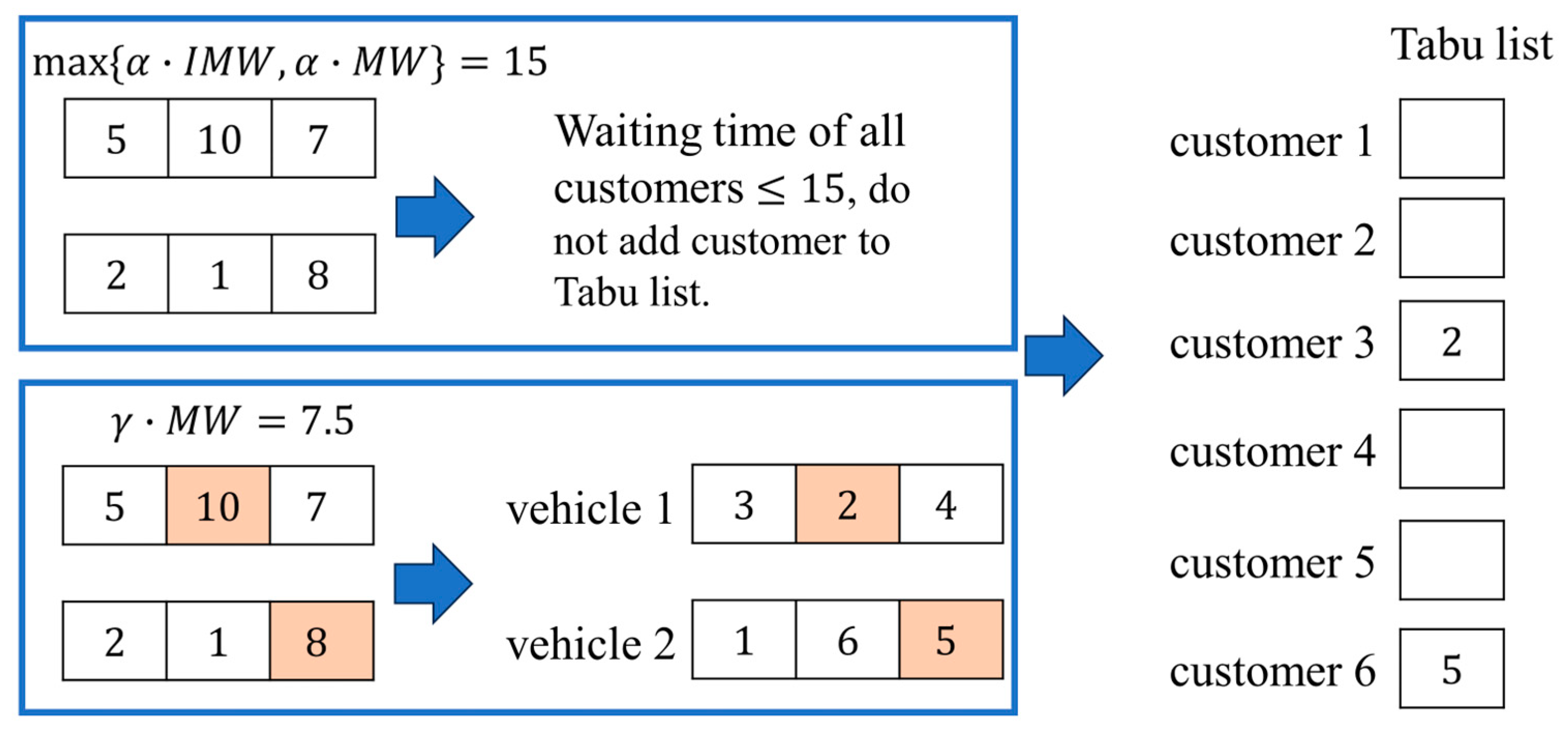
The aim of Phase 2 is to improve the solution from Phase 1 by reducing the waiting time of each vehicle. The solution obtained from Phase 1 is denoted as the current best solution and the objective function value (the sum of the vehicles’ total completion times) is calculated as

$$z={\displaystyle \sum }_{t=1}^k{f}_t$$

In addition to the objective functions mentioned in this research, other types of objective functions can be considered, e.g., finding the shortest distance, minimizing imbalances in routes, or minimizing the penalties for early or late arrivals at customer locations.

The solution improving process consists of three procedures: constructing the tabu list, removing random customers from the sequence, and reconstructing the customer sequence. In creating a tabu list for the objective function of minimizing the sum of the vehicles’ total completion times, it was found that incorporating waiting time yielded the most improved solutions. This is because reducing waiting time leads to the lower total completion time. If the objective function changes, the authors recommend adjusting the conditions for constructing the tabu list to match the new objective function.

The tabu list in this work is a list of forbidden connecting nodes for a customer node. The tabu list of customers $n$ is denoted as $T{L}_n$. The waiting time of customers is then considered, which is the absolute difference between arrival time $\left(a_n\right)$ and available time $(r_n)$ of customer $n$, denoted as $W_n$, that is, $W_n=\left|a_n-r_n\right|$. The maximal waiting time of the initial solution is denoted as $IMW$ and the maximal waiting time as $MW=\max \left\{W_n\right\}$. The tabu list is constructed by adding customers having a waiting time over $\max \left\{\alpha ·IMW,\alpha ·MW\right\}$ where $\alpha \in \left(0,1\right)$.

Besides the conditions mentioned above, the tabu list is constructed by adding the customer having the maximal waiting time and the waiting time over $\gamma ·MW$ where $\gamma$ is a predetermined value between $0<\gamma <\alpha$. For example, suppose the sequence set of customers on vehicle 1 and 2 is $V_1=\left\{3, 2, 4 \right\}$ and $V_2=\left\{1, 6, 5\right\}$, $IMW=15$, the sequence of waiting time of customers 1 to 6 is $W=\left\{W_1, W_2, W_3, W_4, W_5, W_6 \right\}=\left\{2,10, 5, 7, 8,1\right\}$, and set$\alpha =1$ and $\gamma =0.75$. Then, $\max \left\{\alpha ·IMW,\alpha ·MW\right\}=\max \left\{15,10\right\}.$ It is easy to see that the values of $W_2$ and $W_5$ are over $\gamma ·MW=0.75·10=7.5$, as shown in Figure 1.

Since customer 2 is connected to customer 3 in vehicle 1 and customer 5 is connected to customer 6 in vehicle 2, customer 2 and customer 5 will be added to the tabu list of customers 3 and 6, respectively. The tabu list now becomes $T{L}_3=\left\{2\right\}$ and $T{L}_6=\left\{5\right\}$ meaning customer 2 cannot connect to customer 3 while customer 5 also cannot connect to customer 6. $T{L}_1=T{L}_2=T{L}_4=T{L}_5=\varnothing$ means there is no tabu list on customers 1, 2, 4, and 5, as shown in Figure 2.

Function: Tabu list

$\mathbf{Input}:\mathrm{Sequence}\mathrm{set}\mathrm{of}\mathrm{customers}\mathrm{in}\mathrm{all}\mathrm{vehicles}(V_k)$$,\mathrm{tabu}\mathrm{list}\mathrm{of}\mathrm{all}\mathrm{customers}\left(T{L}_i\right)$$,\mathrm{and}\mathrm{the}\mathrm{available}\mathrm{time}\mathrm{for}\mathrm{customer}i$$\left(r_i\right)$$,\mathrm{cut}-\mathrm{off}\mathrm{limit}1\left(\alpha \right)$$,\mathrm{cut}-\mathrm{off}\mathrm{limit}2\left(\gamma \right)$, and $IMW$. $\mathbf{Result}\mathbf{:}\mathrm{Tabu}\mathrm{list}\mathrm{of}\mathrm{all}\mathrm{customers} (T{L}_i).$ $\mathrm{Calculate}\mathrm{the}\mathrm{waiting}\mathrm{time}\mathrm{of}\mathrm{all}\mathrm{customers},W_i=\left|a_i-r_i\right|, i=1,2,3,\dots ,n$. $\mathrm{Find}\mathrm{the}\mathrm{customer}i$$\mathrm{that}\mathrm{has}\mathrm{a}\max \mathrm{waiting}\mathrm{time}.$ $\mathbf{If}{W}_i\ge \max \left\{\alpha ·IMW,\alpha ·MW\right\}$ $\mathrm{Update}\mathrm{the}\mathrm{tabu}\mathrm{list}\mathrm{of}\mathrm{customer}j$$\mathrm{where}j$$\mathrm{is}\mathrm{the}\mathrm{customer}\mathrm{right}\mathrm{before}\mathrm{customer}i$$,T{L}_j=T{L}_j\cup \left\{i\right\}$. End Check the waiting times of all customers. $\mathbf{For}\mathbf{:}i=1ton$ $\mathbf{If} W_i\ge \mathsf{\gamma }·MW$ $\mathrm{Update}\mathrm{the}\mathrm{tabu}\mathrm{list}\mathrm{of}\mathrm{customer}j$$\mathrm{where}j$$\mathrm{is}\mathrm{the}\mathrm{customer}\mathrm{right}\mathrm{before}\mathrm{customer}i$$,T{L}_j=T{L}_j\cup \left\{i\right\}$. End End

To remove a random customer from the sequence, there are three probability options to consider. The first option is to randomly remove a customer based on their waiting time. The longer the waiting time, the more likely the customer is to be removed. This idea arises from the notion that longer customer waiting times are more likely to result in solutions with higher objective function values.

We therefore create the probability of removing a customer with a higher waiting time to be more than that with a lower waiting time. Let the probability of removing customer $j$ ($p_j^1$) be the waiting time of customer $j$ $(W_j)$ divided by the total waiting time of all customers, i.e.,

$$p_j^1={\displaystyle \frac{W_j}{{{\displaystyle \sum }}_{i=1}^n{W}_i}}, j=1,2,\dots ,n$$

The second option is to remove customers with long travel times. This idea arises from the observation that the longer the travel time for a customer, the more likely the solution will yield a higher objective function value. To implement this approach, we create a probability of removing a customer based on their travel time. Let the probability of removing a customer $j$ ($p_j^2$) be the travel time of the vehicle to customer $j$ divided by the total travel time of the system, i.e.,

$$p_j^2={\displaystyle \frac{travel time to customer j}{total travel time}}={\displaystyle \frac{{{\displaystyle \sum }}_{k=1}^m{{\displaystyle \sum }}_{i=1}^n{c}_{ij}{x}_{ij}^k}{{{\displaystyle \sum }}_{k=1}^m{{\displaystyle \sum }}_{i=1}^n{{\displaystyle \sum }}_{l=1}^n{c}_{il}{x}_{il}^k}}, j=1, 2,\dots ,n$$

For the third option, we combine elements from the two previous options and implement a random selection between options one and two. When removing a random customer from the sequence, the selected customer and all its successors will be removed from the route. This process will continue until a predetermined number of customers has been removed, which is calculated as the product of the removal ratio $\left(rm\right)$, and the total number of customers $\left(n\right)$.

Function: Remove customers

$\mathbf{Input}:\mathrm{Sequence}\mathrm{set}\mathrm{of}\mathrm{customers}\mathrm{in}\mathrm{all}\mathrm{vehicles}(V_k$$),\mathrm{probability}\mathrm{options}(Popt$$),\mathrm{removal}\mathrm{ratio}\left(rm\right)$$,\mathrm{the}\mathrm{travel}\mathrm{time}\mathrm{or}\mathrm{distance}\mathrm{from}\mathrm{the}\mathrm{customer}i$$\mathrm{to}\mathrm{customer}j$$(c_{ij}$). $\mathbf{Result}\mathbf{:}\mathrm{Sequence}\mathrm{set}\mathrm{of}\mathrm{customers}\mathrm{in}\mathrm{all}\mathrm{vehicles},V_k$$\mathrm{and}\mathrm{set}\mathrm{of}\mathrm{unassigned}\mathrm{customers}(UC$). $\mathrm{Set}UC=\varnothing .$ $\mathbf{For}\mathbf{:}j=1 to n$ $\mathrm{Calculate}\mathrm{the}\mathrm{removing}\mathrm{probabilities}{p}_j^1={\displaystyle \frac{W_j}{{{\displaystyle \sum }}_{i=1}^n{W}_i}}$$\mathrm{and}{p}_j^2={\displaystyle \frac{{{\displaystyle \sum }}_{k=1}^m{{\displaystyle \sum }}_{i=1}^n{c}_{ij}{x}_{ij}^k}{{{\displaystyle \sum }}_{k=1}^m{{\displaystyle \sum }}_{i=1}^n{{\displaystyle \sum }}_{l=1}^n{c}_{il}{x}_{il}^k}}$. End $\mathbf{For}\mathbf{:}i=1 to [ rm·n]$ $\mathbf{If}Popt=1$ $\mathrm{Randomly}\mathrm{select}\mathrm{customer}j$$\mathrm{using}{p}_j^1$. $\mathbf{Else}\mathbf{If}Popt=2$ $\mathrm{Randomly}\mathrm{select}\mathrm{customer}j$$\mathrm{using}{p}_j^2$. $\mathbf{Else}\mathbf{If}Popt=3$ $\mathrm{Randomly}\mathrm{select}\mathrm{customer}j$$\mathrm{using}\mathrm{random}\mathrm{select}\mathrm{between}Popt=1$$\mathrm{and}Popt=2$. End $\mathrm{Find}{V}_k$$\mathrm{that}\mathrm{contains}j$. $\mathrm{Denote}CP$$\mathrm{as}\mathrm{a}\mathrm{set}\mathrm{of}\mathrm{successors}\mathrm{of}j$$\mathrm{in}\mathrm{the}\mathrm{sequence}\mathrm{set} V_k$. $\mathrm{Remove}\mathrm{customer}j$$\mathrm{and}CP$$\mathrm{from}{V}_k,V_k=V_k-\left(\left\{j\right\}\cup CP\right)$. $\mathrm{Update}\mathrm{set}\mathrm{of}\mathrm{unassigned}\mathrm{customers},UC=UC\cup \left\{j\right\}\cup CP$. End

To reconstruct the customer sequence, the process is executed using the same assignment strategies as in Phase 1. This time, however, the tabu list constraints are strictly enforced to avoid any assigned customer sequences. The algorithm iteratively reconstructs and evaluates the routes, calculating the objective value. If the new solution improves upon the current best solution, it becomes the best-known solution. This iterative process continues until the predetermined number of iterations is reached.

To summarize, our proposed algorithm consists of two phases: initialization phase and solution improvement phase. A summary flowchart is presented in Figure 3. In Phase 1, we obtain a feasible initial solution by assigning the earliest finish time for each customer to the corresponding vehicle. Phase 2 focuses on enhancing the solution generated in Phase 1. During this phase, we consider the waiting time and travel time between two customers as gaps that allow for the removal of some customers. We then construct new routes using a random search method.

4. Simulation Results and Discussion

The objective functions vary across different studies, which means that the solutions from previous work cannot be directly compared to ours. However, we did compare the results obtained by our proposed algorithm with those generated by a solver for small instances. Given that the VRPTW-CT is NP-hard, only small-sized instances can be solved within a reasonable timeframe. To pursue the optimal solution, we modeled the VRPTW-CT using the Julia programming language and solved it using CPLEX.

The well-known Solomon benchmarks with 25 customers are executed on Intel(R) Core (TM) i9 processors with a CPU clock speed of 3.20 GHz and RAM of 192 GB. Note that Solomon’s benchmarks are classified into 6 classes: C1, C2, R1, R2, RC1, and RC2 where nodes in C1 and C2 instances are clustered, while those in R1 and R2 are random, and those in RC1 and RC2 are randomly clustered (combinations of clustered and random customers). We tested 17 clustered-type problems, 23 random-type problems, and 16 random- and clustered-type problems by solving the VRPTW-CT. Recall that the objective function of the VRPTW-CT is to minimize total completion time. Shown in the fourth column of

Table 2. The best solutions of small instances obtained from the VRPTW-CT model via the solver compared with solutions obtained from our proposed algorithm.

Problem	Solutions from the VRPTW-CT Model via Solver			Solutions from the Proposed Algorithm			%Gap
	Number of Vehicles	Total Travel Time	Total Completion Time	Number of Vehicles	Total Travel Time	Total Completion Time
C101	3	295.06	2624.01 *	3	295.06	2624.01	0.00
C102	3	239.50	2506.20	3	254.67	2521.30	0.60
C103	3	271.20	2527.80	3	262.62	2518.73	−0.36
C104	3	293.50	2559.50	3	299.03	2556.95	−0.10
C105	3	275.10	2530.20 *	3	286.02	2537.28	0.26
C106	3	295.06	2630.01 *	3	295.06	2630.01	0.00
C107	3	236.90	2490.70	3	194.77	2444.80	−1.84
C108	3	239.30	2489.50	3	215.80	2465.80	−0.95
C109	3	224.90	2474.90	3	200.22	2450.20	−1.00
C201	2	356.14	3195.27 *	2	328.90	3215.40	0.63
C202	1	305.31	2989.41 *	1	323.92	2989.41	0.00
C203	2	516.12	3099.41 *	2	362.45	3099.41	0.00
C204	1	570.00	2988.60 *	1	300.35	2988.60	0.00
C205	1	326.90	3005.27 *	1	336.80	3005.27	0.00
C206	1	335.58	2989.68 *	1	336.04	2989.68	0.00
C207	1	299.20	2824.70 *	1	294.65	2837.80	0.46
C208	1	347.19	2845.27 *	1	336.80	2845.27	0.00
R101	8	685.95	1295.01 *	8	708.07	1295.01	0.00
R102	7	741.90	1188.70	7	786.04	1172.70	−1.35
R103	4	535.30	793.30	4	545.72	837.22	5.54
R104	4	511.80	761.80	4	464.70	778.59	2.20
R105	5	560.10	930.10 *	5	582.46	957.33	2.93
R106	5	627.40	877.40	5	578.48	888.46	1.26
R107	4	539.70	789.70	4	504.73	764.17	−3.23
R108	4	447.40	697.70	4	475.89	758.78	8.80
R109	4	469.10	762.30	4	479.48	780.93	2.44
R110	5	498.10	766.70	5	514.71	783.06	2.13
R111	5	511.80	794.50	5	564.85	841.87	5.96
R112	4	426.40	691.20	4	448.78	713.65	3.25
R201	2	772.80	1345.90 *	2	821.74	1348.13	0.17
R202	2	745.00	1322.20	2	726.81	1342.54	1.54
R203	3	964.60	1341.10	1	660.82	1303.61	−2.80
R204	1	635.50	885.50	1	565.63	860.54	−2.82
R205	1	559.40	846.00 *	1	579.24	848.02	0.24
R206	1	582.10	832.10	1	533.14	830.00	−0.25
R207	1	570.10	820.10	1	535.76	805.36	−1.80
R208	1	525.20	775.20	1	411.98	782.54	0.95
R209	1	488.20	756.00	1	484.46	738.65	−2.29
R210	2	634.40	909.50 *	2	744.91	1119.00	23.03
R211	2	481.10	734.30	1	466.65	724.01	−1.40
RC101	4	492.10	796.90 *	4	488.48	801.65	0.60
RC102	3	369.30	629.70 *	3	358.83	631.67	0.31
RC103	4	466.70	731.10	4	374.66	632.99	−13.42
RC104	4	455.70	705.70	3	366.67	619.87	−12.16
RC105	4	441.50	759.10 *	4	495.92	811.54	6.91
RC106	3	354.30	614.90 *	3	361.62	625.37	1.70
RC107	3	305.00	566.70	3	324.19	575.86	1.62
RC108	7	580.30	831.00	3	321.86	571.86	−31.18
RC201	2	813.10	1295.30 *	2	739.59	1396.00	7.77
RC202	2	641.00	934.20	2	829.55	1264.50	35.36
RC203	1	600.20	850.20 *	1	570.72	878.42	3.32
RC204	1	591.10	841.10	1	462.87	852.58	1.36
RC205	2	767.30	1314.40	2	855.80	1596.30	21.45
RC206	1	571.50	831.70	1	562.47	856.41	2.97
RC207	2	604.00	883.90	2	674.63	1106.00	25.13
RC208	1	394.40	659.80	1	394.08	673.01	2.00

* Optimal solution with the relative gap is equal to zero where relative gap $=\left|UB-LB\right|/UB.$ Optimal solutions obtained from our algorithm are appeared in bold.

, below, is the optimal solution found, with the number of occupied vehicles shown in the second column. The travel time associated with these solutions is calculated and shown in the third column. Also shown in Table 2 are the results obtained with our proposed algorithm where the number of vehicles, travel time, and completion time are in the fifth–seventh columns, respectively. The %Gap of total completion time appears in the last column where %Gap is calculated by the following:

$$\%\mathrm{Gap}={\displaystyle \frac{{\mathrm{Total}\mathrm{Completion}\mathrm{time}}_{\mathrm{Alg}}-{\mathrm{Total}\mathrm{Completion}\mathrm{time}}_{\mathrm{model}}}{{\mathrm{Total}\mathrm{Completion}\mathrm{time}}_{\mathrm{model}}}}\times 100$$

As shown in Table 2, there are 21 problems where the optimal solutions can be found by solving the VRPTW-CT directly. In nine problems, the optimal solutions are reached via our proposed algorithm. When comparing routes between the optimal solutions obtained from the VRPTW-CT and with our proposed algorithm, the same routes are found in instances C101 and C106, while different routes with the same objective function values are found in instances C202, C203, C204, C205, C206, C208, and R101. The optimal routing of instance C101 obtained with our algorithm is shown in Figure 4. Figure 5a,b show the optimal solutions of instance C203 obtained from solving the VRPTW-CT model and our proposed algorithm, respectively. Note that the same group of customers is served by the same vehicle in a different order. In Figure 6a,b, the optimal solutions of R101 were obtained from solving the VRPTW-CT and with our algorithm, respectively. In this case, the optimal solutions show some vehicles serving different groups of customers.

Observe that %Gap in some problems are negative values. This is because the optimal solutions are not reached in those problems.

It is worth mentioning that in problems C205 and C208, the solution obtained from Phase 1 of the proposed algorithm is optimal. In minimizing the total travel time, customers in the same cluster will logically be served by the same vehicle if the time windows are not violated. We observed that when minimizing the total completion time, some customers in the same cluster will be served by different vehicles in the optimal solution. This is because the earliest finish time of the customer will be assigned to the vehicle. The execution times of solving cluster instances (C1 and C2), random instances (R1 and R2), and randomly clustered instances (RC1 and RC2) range between 2 and 300, 60 and 10,000, and 1000 and 20,000 s, respectively. Some problems require a long execution time to obtain optimal solutions because the lower bounds of the problem are not updated.

To demonstrate algorithm effectiveness on larger problems, we tested our algorithm using Solomon instances featuring 100 customers. The total completion time of each problem is shown in the fourth column while the corresponding total travel time is calculated and shown in the third column of

Table 3. The optimal solution of large instances obtained with our algorithm.

Problem	Number of Vehicle	Total Travel Time	Total Completion Time
C101	10	828.94	9828.94
C102	10	1308.04	10,361.40
C103	11	1556.45	10,629.86
C104	10	1425.82	10,425.82
C105	11	1598.83	10,671.81
C106	10	932.80	9932.80
C107	10	831.02	9831.02
C108	11	941.44	9944.63
C109	13	1321.20	10,337.65
C201	3	591.56	9591.56
C202	4	1404.67	10,614.11
C203	4	1890.17	11,417.00
C204	4	1783.91	10,799.84
C205	3	608.33	9608.33
C206	4	1235.55	10,237.43
C207	5	1185.40	10,197.63
C208	4	640.25	9640.25
R101	19	1854.85	3407.07
R102	19	2024.31	3266.04
R103	17	1816.90	2889.36
R104	13	1322.29	2393.69
R105	15	1493.63	2732.52
R106	13	1473.01	2523.85
R107	13	1280.12	2426.15
R108	10	1125.96	2127.89
R109	13	1283.96	2414.51
R110	12	1299.70	2339.74
R111	12	1320.35	2340.58
R112	11	1166.59	2170.96
R201	4	1937.61	3065.54
R202	5	1689.47	2940.95
R203	5	1691.89	3022.30
R204	4	1463.51	2512.12
R205	5	1721.71	2751.49
R206	5	1533.32	2550.57
R207	5	1532.94	2537.42
R208	5	1492.52	2492.52
R209	4	1517.72	2531.41
R210	4	1745.09	2793.51
R211	4	1414.35	2416.48
RC101	18	2060.39	3389.19
RC102	16	1866.77	2965.84
RC103	14	1737.67	2802.98
RC104	14	1590.34	2591.88
RC105	18	2060.39	3389.19
RC106	15	1718.74	2826.07
RC107	14	1618.48	2643.77
RC108	13	1603.14	2608.84
RC201	5	2312.12	3431.47
RC202	5	2133.43	3214.11
RC203	6	2004.32	3116.71
RC204	6	1828.10	2936.37
RC205	5	2243.16	3391.28
RC206	6	1981.53	3089.99
RC207	7	2606.09	3619.32
RC208	4	1874.88	2891.81

. The number of vehicles used to serve customers is shown in the second column. Result comparison with the existing algorithm cannot be done because of the different objective functions.

5. Real-World Application

Recently, the Department of Medical Services of Thailand has implemented a policy to promote Personal-Based Medical Services, leading to the establishment of home ward programs which aim to visit patients at home to help reduce hospital congestion, and improve overall healthcare accessibility and quality in Thailand [42]. The completion time for caregivers is often used as a benchmark to effectively manage the HHC services. To illustrate the advantages of the proposed algorithm with real-world application, this work addresses minimizing the total completion time of caregivers in an HHC problem. The completion time in our context consists of the total travel time, including return time to the healthcare center, the waiting time, and the service time. In 2023, Saksuriya and Likasiri [23] proposed a mathematical model and algorithm for solving an HHC system, using one in Chiang Mai, Thailand as the case study. Their objective function was minimizing the customers’ completion time which excludes the caregivers’ return time to the healthcare center. We employ their case study consisting of 400 customers who need HHC services from a single center. The available time, end time, and service time are randomized. The travel time between two customers is collected using Google Maps. The working hours of each caregiver are assumed not to exceed 8 h. In this study, the primary objective of our proposed algorithm is to minimize the sum of caregivers’ total completion times. The second and third objective functions are here to compare the solutions with the existing algorithm. Our algorithm can thus pivot according to these three objective functions: (1) the total completion time of all caregivers which includes return time to the healthcare center, (2) the total completion time of all customers which excludes return time to the healthcare center, and (3) the total travel time. The solutions under the three objective functions shown in

Table 4. Results obtained from Saksuriya and Likasiri [23] compared to solutions obtained with our proposed algorithm.

Solution	# Caregiver	Number of Customers per Caregiver			Completion Time Excluding Return Time per Caregiver (Hours)			Travel Time per Caregiver (Hours)			Total Completion time Excluding Return Time (Hours)	Total Completion Time Including Return Time (Hours)
		Min	Max	Avg	Min	Max	Avg	Min	Max	Avg
[23]	34	8	18	11.7	1.5	6.9	4.4	1.3	2.2	1.5	N/A	N/A
Obj. 1	14	12	60	28.6	6.9	7.9	7.6	1.7	4.0	2.4	107.1	110.8
Obj. 2	14	8	60	28.6	7.4	7.9	7.7	1.8	4.3	2.4	107.4	110.6
Obj. 3	14	13	60	28.6	7.4	7.8	7.6	1.7	4.0	2.3	106.6	110.5

. One can see that all results obtained with our proposed algorithm require fewer caregivers than those obtained in [23]. In fact, there are 14 caregivers required in our proposed algorithm while 34 caregivers are required in [23]. This solution will reduce expenses on caregivers, thereby lowering government costs associated with the HHC system. Furthermore, by decreasing hospital visits, it will minimize the risk of older adults being exposed to other diseases. However, by observing the average number of customers per caregiver we found that in our solution, every caregiver must serve more customers than the number obtained in [23], resulting in longer work time for each caregiver. When completion times are compared side by side, the caregivers working time obtained with our proposed algorithm is more balanced than that from [23]. Our findings indicate that the number of caregivers identified by our algorithm is fewer than the number reported in [23]. Additionally, the workload for all caregivers is nearly equal to the maximum allowable working hours. These results are conducive to the management of the HHC system. In general, after all caregivers serve all customers, they must return to the healthcare center. The last column displays the total completion time which includes return time to the healthcare center obtained with our algorithm. When comparing the travel times of each caregiver, we note that the average travel time reported in [23] is lower than that generated by our algorithm. This does not guarantee that the total travel time will be lower than that obtained with our algorithm because the number of caregivers yielded in [23] is more than that yielded by our algorithm. Shown in Figure 7 is the best result of our algorithm when finding a solution under the third objective function where 400 customers are assigned to 14 caregivers. Here, the 14 caregivers are indicated by 14 different colors and the location points of the same color will be assigned to the same route. Thirteen customers are served by the 14th caregivers (or route 14). That shortest route is also shown in Figure 7. We observe that customers assigned to the 14th caregivers are scattered around the map. Since customers have different available times and our proposed algorithm will prioritize assigning the best completion time to the caregiver, the customer who is assigned may not be in close proximity.

6. Conclusions

In this study, we have developed a mathematical model and algorithms for the VRPTW specifically tailored to an HHC system. The primary objective was to minimize the total completion time by effectively reducing vehicle waiting times. Our approach has shown a significant enhancement in service efficiency through the integration of a modified greedy initialization with a tabu search. The first step of the proposed algorithm is to find the initial feasible solution by assigning customers with the best finish time, then the initial solution is improved by removing and rearranging customers in each route with a different probability. The optimal solutions can be found in some small-sized instances because the VRPTW is NP-hard. To illustrate the performance of the proposed model and algorithm, Solomon’s benchmark instances with 25 customers are tested and comparisons are then made. The efficiency of the proposed algorithm is also shown using Solomon’s benchmark instances with 100 customers. The results indicate that our approach not only decreases the overall completion time but also significantly reduces the waiting time for each customer. Finally, we applied the proposed algorithm to solve an HHC problem in Chiang Mai [23]. Working hours of caregivers do not exceed 8 h in the case study. Results show that the solution obtained with our proposed algorithm employs a smaller number of caregivers than the solution in [23] and each caregiver’s working time falls in the range of 7–8 h. The number of caregivers can be lowered by approximately 59% while the average caregiver completion time falls between 95 and 96% of the 8 h working day. This shows that we can reduce the service costs and that all caregivers’ working hours are almost at the time limit per day. We can manage the working hours for all caregivers to be (1) nearly balanced, and (2) close to their maximum. Therefore, we assert that our algorithm is effective for the HHC management system. Our proposed algorithm has the advantage of being able to pivot under three objective functions: (1) the caregivers’ total completion time which includes the return time to the healthcare center, (2) the customers’ total completion time which excludes the return time of the caregivers, and (3) the total travel time. Moreover, the proposed methodology can be adapted and optimized for broader applications beyond HHC service, including for urban logistics and supply chain management. However, our proposed algorithm unfortunately gets stuck at local optima in some problems due to randomization in certain steps. We suggest modifications to our algorithm for future work to prevent this issue.

References

1. Wy, J.; Kim, B.-I.; Kim, S. The rollon–rolloff waste collection vehicle routing problem with time windows. Eur. J. Oper. Res. 2013, 224, 466–476. [Google Scholar] [CrossRef]
2. Zhang, H.; Zhang, Q.; Ma, L.; Zhang, Z.; Liu, Y. A hybrid ant colony optimization algorithm for a multi-objective vehicle routing problem with flexible time windows. Inform. Sci. 2019, 490, 166–190. [Google Scholar] [CrossRef]
3. Huang, M.; Liu, M.; Kuang, H. Vehicle routing problem for fresh products distribution considering customer satisfaction through adaptive large neighborhood search. Comput. Ind. Eng. 2024, 190, 110022. [Google Scholar] [CrossRef]
4. Gómez S., C.G.; Cruz-Reyes, L.; González B., J.J.; Fraire H., H.J.; Pazos R., R.A.; Martínez P., J.J. Ant colony system with characterization-based heuristics for a bottled-products distribution logistics system. J. Comput. Appl. Math. 2014, 259 Pt B, 965–977. [Google Scholar] [CrossRef]
5. Mamoun, K.A.; Hammadi, L.; Ballouti, A.E.; Novaes, A.G.N.; De Cursi, E.S. Vehicle routing optimization algorithms for pharmaceutical supply chain: A systematic comparison. Transp. Telecommun. J. 2024, 25, 161–173. [Google Scholar] [CrossRef]
6. Somar, S.; Urazel, B.; Sahin, Y.B. A modified metaheuristic algorithm for a home health care routing problem with health team skill levels. Appl. Soft Comput. 2023, 148, 110912. [Google Scholar] [CrossRef]
7. United Nations Population Fund, Ageing. Available online: https://www.unfpa.org/ageing#readmore-expand (accessed on 29 November 2024).
8. World Health Organization, Ageing and Health. Available online: https://www.who.int/news-room/fact-sheets/detail/ageing-and-health (accessed on 28 November 2024).
9. Population Reference Bureau, 2024 World Population Data Sheet. Available online: https://2024-wpds.prb.org/wp-content/uploads/2024/09/2024-World-Population-Data-Sheet-Booklet.pdf (accessed on 12 December 2024).
10. Eurostat, Population Structure and Ageing. Available online: https://ec.europa.eu/eurostat/statistics-explained/index.php?title=Population_structure_and_ageing (accessed on 10 December 2024).
11. Economic and Social Commission for Asia and the Pacific (ESCAP), Demographic Changes Asia and the Pacific: Population Ageing Data. Available online: https://www.population-trends-asiapacific.org/data (accessed on 10 December 2024).
12. United Nations, Thailand Economic Focus: Demographic Change in Thailand: How Planners Can Prepare for the Future. Available online: https://thailand.un.org/en/96303-thailand-economic-focus-demographic-change-thailand-how-planners-can-prepare-future (accessed on 29 November 2024).
13. Liu, R.; Xie, X.; Augusto, V.; Rodriguez, C. Heuristic algorithms for a vehicle routing problem with simultaneous delivery and pickup and time windows in home health care. Eur. J. Oper. Res. 2013, 230, 475–486. [Google Scholar] [CrossRef]
14. Haddadene, S.R.A.; Labadie, N.; Prodhon, C. A GRASP × ILS for the vehicle routing problem with time windows, synchronization and precedence constraints. Expert Syst. Appl. 2016, 66, 274–294. [Google Scholar] [CrossRef]
15. Liu, R.; Yuan, B.; Jiang, Z. A branch and price algorithm for the home caregiver scheduling and routing problem with stochastic travel and service times. Flex. Serv. Manuf. J. 2019, 31, 989–1011. [Google Scholar] [CrossRef]
16. Euchi, J.; Zidi, S.; Laouamer, L. A Hybrid Approach to Solve the Vehicle Routing Problem with Time Windows and Synchronized Visits In-Home Health Care. Arab. J. Sci. Eng. 2020, 45, 10637–10652. [Google Scholar] [CrossRef]
17. Chaieb, M.; Sassi, D.B. Measuring and evaluating the Home Health Care Scheduling Problem. Appl. Soft Comput. 2021, 113, 107957. [Google Scholar] [CrossRef]
18. Makboul, S.; Kharraja, S.; Abbassi, A.; Alaoui, A.E.H. A multiobjective approach for weekly Green Home Health Care routing and scheduling problem with care continuity and synchronized services. Oper. Res. Perspect. 2024, 12, 100302. [Google Scholar] [CrossRef]
19. Baños, R.; Ortega, J.; Gil, C.; Fernández, A.; de Toro, F. A Simulated Annealing-based parallel multi-objective approach to vehicle routing problems with time windows. Expert Syst. Appl. 2013, 40, 1696–1707. [Google Scholar] [CrossRef]
20. Hifi, M.; Wu, L. A hybrid metaheuristic for the Vehicle Routing Problem with Time Windows. In Proceedings of the International Conference on Control, Decision and Information Technologies (CoDIT), Metz, France, 3–5 November 2014. [Google Scholar] [CrossRef]
21. François, V.; Arda, Y.; Crama, Y. Adaptive Large Neighborhood Search for Multitrip Vehicle Routing with Time Windows. Transp. Sci. 2019, 53, 1706–1730. [Google Scholar] [CrossRef]
22. Ahmed, Z.H.; Maleki, F.; Yousefikhoshbakht, M.; Haron, H. Solving the vehicle routing problem with time windows using modified football game algorithm. Egypt. Inform. J. 2023, 24, 100403. [Google Scholar] [CrossRef]
23. Saksuriya, P.; Likasiri, C. Vehicle Routing Problem with Time Windows to Minimize Total Completion Time in Home Healthcare Systems. Mathematics 2023, 11, 4846. [Google Scholar] [CrossRef]
24. Yue, B.; Yang, J.; Ma, J.; Shi, J.; Shangguan, L. An improved sequential insertion algorithm and tabu search to vehicle routing problem with time windows. RAIRO Oper. Res. 2024, 58, 1979–1999. [Google Scholar] [CrossRef]
25. Solomon, M.M. Algorithms for the Vehicle Routing and Scheduling Problems with Time Window Constraints. Oper. Res. 1987, 35, 254–265. [Google Scholar] [CrossRef]
26. Kallehauge, B.; Larsen, J.; Madsen, O.B.G.; Solomon, M.M. Vehicle Routing Problem with Time Windows. In Column Generation; Desaulniers, G., Desrosiers, J., Solomon, M.M., Eds.; Springer: Boston, MA, USA, 2005; pp. 67–98. [Google Scholar]
27. Bräysy, O.; Gendreau, M. Vehicle Routing Problem with Time Windows, Part I: Route Construction and Local Search Algorithms. Transp. Sci. 2005, 39, 104–118. [Google Scholar] [CrossRef]
28. Bräysy, O.; Gendreau, M. Vehicle Routing Problem with Time Windows, Part II: Metaheuristics. Transp. Sci. 2005, 39, 119–139. [Google Scholar] [CrossRef]
29. Gehring, H.; Homberger, J. A Parallel Hybrid Evolutionary Metaheuristic for the Vehicle Routing Problem with Time Windows. Available online: https://citeseerx.ist.psu.edu/document?repid=rep1&type=pdf&doi=e41b80d075429403f569980d278f6d4f91da2594 (accessed on 26 May 2025).
30. Zong, Z.; Tong, X.; Zheng, M.; Li, Y. Reinforcement Learning for Solving Multiple Vehicle Routing Problem with Time Window. ACM Trans. Intell. Syst. Technol. 2024, 15, 32. [Google Scholar] [CrossRef]
31. Bent, R.; Hentenryck, P.V. A two-stage hybrid algorithm for pickup and delivery vehicle routing problems with time windows. Comput. Oper. Res. 2006, 33, 875–893. [Google Scholar] [CrossRef]
32. Vidal, T.; Crainic, T.G.; Gendreau, M.; Prins, C. A hybrid genetic algorithm with adaptive diversity management for a large class of vehicle routing problems with time-windows. Comput. Oper. Res. 2013, 40, 475–489. [Google Scholar] [CrossRef]
33. Gmira, M.; Gendreau, M.; Lodi, A.; Potvin, J.-Y. Tabu search for the time-dependent vehicle routing problem with time windows on a road network. Eur. J. Oper. Res. 2021, 288, 129–140. [Google Scholar] [CrossRef]
34. Wang, H.-F.; Chen, Y.-Y. A genetic algorithm for the simultaneous delivery and pickup problems with time window. Comput. Ind. Eng. 2012, 62, 84–95. [Google Scholar] [CrossRef]
35. Srivastava, G.; Singh, A.; Mallipeddi, R. NSGA-II with objective-specific variation operators for multiobjective vehicle routing problem with time windows. Expert Syst. Appl. 2021, 176, 114779. [Google Scholar] [CrossRef]
36. Melián-Batista, B.; Santiago, A.D.; AngelBello, F.; Alvarez, A. A bi-objective vehicle routing problem with time windows: A real case in Tenerife. Appl. Soft Comput. 2014, 17, 140–152. [Google Scholar] [CrossRef]
37. Eydi, A.; Ghasemi-Nezhad, S.A. A bi-objective vehicle routing problem with time windows and multiple demands. Ain Shams Eng. J. 2021, 12, 2617–2630. [Google Scholar] [CrossRef]
38. Schneider, M.; Stenger, A.; Goeke, D. The Electric Vehicle-Routing Problem with Time Windows and Recharging Stations. Transp. Sci. 2014, 48, 500–520. [Google Scholar] [CrossRef]
39. Erdelić, T.; Carić, T. Goods Delivery with Electric Vehicles: Electric Vehicle Routing Optimization with Time Windows and Partial or Full Recharge. Energies 2022, 15, 285. [Google Scholar] [CrossRef]
40. Luo, T.; Heng, Y.; Xing, L.; Ren, T.; Li, Q.; Qin, H.; Hou, Y.; Wang, K. A Two-Stage Approach for Electric Vehicle Routing Problem with Time Windows and Heterogeneous Recharging Stations. Tsinghua Sci. Technol. 2024, 29, 1300–1322. [Google Scholar] [CrossRef]
41. Smith, W.E. Various optimizers for single-stage production. Nav. Res. Logist. Q. 1956, 31, 59–66. [Google Scholar] [CrossRef]
42. Department of Medical Services, Home Ward Standard and Guidelines. Available online: https://www.dms.go.th/backend//Content/Content_File/Publication/Attach/25650805113031AM_homeward.pdf (accessed on 26 May 2025). (In Thai).
Figure 1. Process of finding maximum waiting time.
Logistics 09 00085 g001
Figure 2. Process of constructing the tabu list for each customer.
Logistics 09 00085 g002
Figure 3. The flowchart of the proposed algorithm.
Logistics 09 00085 g003
Figure 4. The optimal solutions of C101 obtained from the VRPTW-CT model by using solver and with our proposed algorithm.
Logistics 09 00085 g004
Figure 5. Different optimal solutions of C203 instance obtained from (a) the VRPTW-CT model and (b) our proposed algorithm.
Logistics 09 00085 g005
Figure 6. Different optimal solutions of R101 instance obtained from (a) the VRPTW-CT model and (b) our proposed algorithm.
Logistics 09 00085 g006
Figure 7. The best solution from our proposed algorithm with the caregiver serving a minimum number of customers.
Logistics 09 00085 g007