Integrated Economic and Environmental Dimensions in the Strategic and Tactical Optimization of Perishable Food Supply Chain: Application to an Ethiopian Real Case

Abstract

Background: The agri-food sector is a major contributor to environmental degradation and emissions, highlighting the need for sustainable practices to mitigate its impact. Within this sector, perishable food crops require targeted efforts to reduce their environmental footprint. Vertical integration is crucial for ensuring alignment between strategic and tactical decision making in supply chain management. This article presents a multi-objective mathematical model that integrates both economic and environmental considerations within the perishable food supply chain, aiming to determine optimal solutions for conflicting objectives. Methods: In this research, we employed combining goal programming with the epsilon constraint approach; this comprehensive methodology reveals optimal solutions by discretizing the values derived from the payoff table. Results: The model is applied to a real case study of the tomato paste supply chain in Ethiopia. To identify Pareto-efficient points, the results are presented in two scenarios: Case I and Case II. Conclusions: The findings emphasize the significant influence of the geographical location of manufacturing centers in supplier selection, which helps optimize the trade-off between environmental impact and total cost. The proposed solution provides decision makers with an effective strategy to optimize both total cost and eco-costs in the design of perishable food supply chain networks.

1. Introduction

In the food supply chain, perishable raw materials such as fruits, vegetables, and dairy products play a crucial role. These products, however, face inherent challenges due to their limited shelf life. The logistics of these products often require energy-intensive means, such as refrigeration and frequent transportation, leading to greenhouse gas (GHG) emissions, contributing to approximately 25% of the total emissions worldwide [1]. Thus, reducing the impacts of the agri-food sector is one of the foremost priorities within the European Sustainable Production and Consumption policies [2].

In many developing countries like Ethiopia, fragmented production system marked by smallholder dominance, dispersed collection points, and inadequate storage and processing infrastructure combined with the high capital demands of modern processing facilities has impeded the development of a competitive food-processing industry. Despite Ethiopia’s significant agricultural potential, the development of a robust perishable food processing industry remains severely constrained. Investment shortfalls have left only a handful of medium- to large-scale processors operational, preventing the realization of economies of scale necessary to meet the country’s growing domestic demand. For instance, the Merti Agro-Processing Plant, one of Ethiopia’s largest tomato processors, operates with an annual processing capacity of only 3000 metric tons, which falls far short of satisfying national consumption needs (Ministry of Agriculture, 2019 [3]). As a result, reliance on imported tomato products has steadily increased, with over 4000 metric tons imported during the 2021/22 fiscal year alone (Ethiopian Customs Authority, 2022). This persistent gap between limited domestic production and rising consumer demand underscores critical structural weaknesses in both processing capacity and upstream supply chain infrastructure. Addressing these challenges requires integrated investments in processing facilities, collection centers, cold storage systems, and transportation networks to enhance the efficiency, competitiveness, and self-sufficiency of Ethiopia’s perishable food sector.

Mapping potential production zones based on raw-material availability, proximity to rapidly urbanizing centers, and environmental considerations offers a strategic pathway for the Ethiopian government to establish a robust raw material processing sector. Such efforts can enhance food security, promote environmental sustainability, and reduce import dependency. Effective site selection is crucial, as it supports the growth of the horticultural industry while enabling the scaling up of tomato processing operations in regions best suited for consistent supply with minimal ecological impact. Despite strong government interest and favorable geographic and climatic conditions, the development of an integrated and optimized agri-food processing sector remains limited. Tomato processing, although prioritized for its production potential, health benefits, and high yield, is used as a case study in this paper as it is still insufficient to meet national demand. This shortfall stems from various challenges within agri-fresh food supply chains (AFFSCs), particularly those related to perishability and supply chain uncertainties. Therefore, addressing these challenges requires more in-depth quantitative research that rigorously employs mathematical models, statistical analyses, and data-driven techniques. This in-depth investigation of inefficiencies within agri-fresh food supply chains (AFFSCs) is essential for informing evidence-based decision making and fostering sectoral growth.

The agri-food sector plays a critical role in the global economy, highlighting the need for advanced decision-making tools to improve efficiency and sustainability across supply chains [4]. In response, many studies have employed optimization models to address specific challenges at either the upstream (e.g., production and sourcing) or downstream (e.g., distribution and retail) stages of these supply chains [5]. However, despite the growing body of research in agri-food supply chain management, there remains a notable gap in the development and application of integrated, system-wide approaches that can support the holistic design and planning of these inherently complex and dynamic networks. This gap in integrated planning is particularly concerning given the scale of food loss globally. An estimated 33% of all food produced each year is lost or wasted, with fruits and vegetables accounting for nearly 70% of this total [6]. Such losses exacerbate global food insecurity by widening the gap between food availability and growing demand, especially in rapidly urbanizing regions. Furthermore, it also contributes significantly to environmental degradation through inefficient use of water, land, and energy, alongside increased greenhouse gas emissions. These realities underscore the urgent need for integrated, optimization-based supply chain planning models that not only mitigate food loss but also enhance sustainability and resilience within agri-food systems. Despite significant research on perishable food supply chains, critical challenges and effective mitigation strategies remain underexplored [7]. This issue has not been adequately addressed in developing countries like Ethiopia, highlighting the need for integrated studies that focus on the unique complexities and constraints involved in managing perishable products in these contexts. Additionally, the lack of available data poses a significant challenge in tackling these issues effectively. It has been emphasized that due to the fundamental differences in production processes and product characteristics, specific models focusing on crop-based or animal-based agri-food supply chains (AFSCs) have not received sufficient attention [4]. This gap highlights the need for tailored approaches that address the unique dynamics of each type of supply chain. One approach to address this issue is to develop a holistic integrated strategic and tactical planning model for plant-based perishable products considering economic and environmental perspectives. Economic and environmental factors are crucial for transforming agri-food value chains sustainably in developing countries [8]. Addressing these factors positively impacts both economic development and environmental protection, as the agricultural sector serves as the backbone of these nations and production potential is enormous.

In this paper, our objective is to expand the understanding of perishable food supply chain management by offering insights that will improve strategic and tactical decisions through the incorporation of environmental aspects within a multi-sourcing strategy. Our principal aim is to develop a mathematical model designed to optimize the entire perishable products supply chain at a national scale, encompassing multi-supplier, multi-manufacturing center, multi-distribution center, and multi-customer networks. This model will ensure economic viability while reflecting real-world conditions. Thus, the central scientific research question we seek to address is as follows: How can the perishable food supply chain be effectively modeled and managed, incorporating environmental dimension within both strategic and tactical planning?

In summary, this study offers the following significant contributions:

• Explores and optimizes multi-sourcing strategies, enabling supply chains to be more resilient and flexible. This approach helps to mitigate risks associated with supply disruptions and ensures continuous product availability by leveraging multiple suppliers.
• Provides actionable insights for decision makers looking to improve the efficiency and reliability of perishable food supply chains in various contexts. The model is tested and validated through a real case study conducted in Ethiopia, demonstrating its practical applicability.
• Combines strategic and tactical decisions to mitigate the adverse effects of uncertainties in decision-making processes and to assess the impact of incorporating environmental dimension within a multi-sourcing strategy supply chain.
• Offers valuable implications for policymakers, particularly in the areas of food security and supply chain resilience, by showing how advanced optimization techniques can be leveraged to support national and regional food distribution networks.
• Regarding the resolution method, we were obliged to develop an integrated ε-constraint and goal programming approach to address the complexity and large scale of the problem, which arises from its application to a country-level case study. This methodological advancement ensures effective handling of multiple objectives while maintaining computational tractability for large, real-world instances.

The structure of the paper is outlined as follows: Section 2 reviews the existing literature on network design challenges specific to perishable food supply chains. Section 3 defines and formulates the problem at hand. Section 4 details the proposed solutions and methodologies. Section 5 presents the results and offers an analysis. Finally, Section 6 concludes with a summary of findings and suggestions for future research.

2. State of the Art

This section explores the latest advancements in perishable food supply chain network design, focusing on the integration of economic and environmental aspects at the strategic and tactical level. Recent developments have led to the creation of different models that address the challenges of managing perishable products, which are particularly vulnerable to time and environmental factors. This overview highlights key findings while also identifying critical gaps and areas for future research to further enhance perishable food supply chain management from an optimization perspective. This analysis does not attempt to cover all attributes of the reviewed models but focuses specifically on those directly related to minimizing cost and environmental impact. For a more detailed examination of optimization models in AFSC design, readers are encouraged to consult [4].

The previous research has concentrated on multi-echelon, multi-period, and multi-product approaches to tackle strategic and operational decisions in perishable food supply chains, addressing key aspects such as production, facility location, resource allocation, inventory, and routing [9]. Order planning involving multiple suppliers, distribution centers, and customers, with an emphasis on a specific type of perishable raw material, represents another important research direction [10]. Additionally, leveraging food hubs in the distribution channel has demonstrated the potential to achieve optimal long-term environmental performance, significantly reducing the carbon footprint across the entire network [11]. Further advancements include addressing the multi-echelon, multi-product, and multi-period production–location–inventory problem within sustainable perishable product supply chains [12]. A framework is proposed to optimize strategic and operational decisions while accounting for disruption risks such as lost demand, storage constraints, and capacity disturbances [13]. Moreover, a novel production routing model is introduced to minimize costs related to production, inventory, routing, product waste, and penalties for reduced freshness [14]. However, they focused solely on the retailer stage. An integrated production routing model at the tactical level also developed, considering factors such as storage temperature and vehicle conditions [15]. Meanwhile, a sourcing–production–inventory (SPI) model for a single manufacturer is developed incorporating sourcing and production decisions under quantity discounts and examining environmental impacts due to spoilage [16].

A nonlinear mixed-integer programming model is developed for a green closed-loop supply chain that manages the complexities of perishable products under uncertain conditions, optimizing production, inventory, and routing decisions [17]. A key element of this innovation is the recognition and integration of the unpredictable nature of perishable products’ lifespans, which enables adaptive decision-making strategies that are resilient to unexpected disruptions and variations in product life cycles. This adaptability is crucial, especially as fluctuations in cash flow resulting from changes in product quality can significantly impact pricing and replenishment strategies [18]. Additionally, a mixed-integer programming (MILP) model supports the order promising process in fruit supply chains by maximizing total profit and mean product freshness while ensuring customer requirements for subtype homogeneity and traceability of product deterioration [19].

The research has also explored various models tailored to the unique challenges of perishable products. For instance, a simulation-based optimization model adapts a discrete choice framework to learn ordering rules for vertically differentiated perishable items, aiming to maximize long-term average profit while considering consumer heterogeneity and the trade-offs between price and quality [20]. The impact of product perishability on agri-food supply chain design is examined through a novel mixed-integer linear programming model [21]. However, it assumes product prices are independent of freshness, which may not align with actual market dynamics. Furthermore, a modeling framework is presented for locating order fulfilment centers near consumers, utilizing population density as a proxy for demand [22]. However, this approach may inadequately capture the complexities of consumer behavior and preferences. The decline in quality of perishable food products is an important consideration when planning hub locations in supply chains [23]. In a related effort, a hybrid model is proposed at strategic and operational levels specifically designed to tackle the complexities of supply chain network design within the horticulture sector [24]. Similarly, the need for various strategic, tactical, and operational issues that account for the deterioration of product quality is proposed [25].

In the realm of sustainability, a bi-objective optimization model addresses the location, inventory, and routing challenges necessary for building a resilient supply network for perishable foods [26]. While this model is promising, it may not fully account for variations in supply chain dynamics, limiting its applicability across different contexts. Other studies emphasize the importance of incorporating perishability and sustainability into decision-making processes [27,28,29]. However, these models often have limitations, such as focusing on specific supply chain configurations or case studies that may restrict broader applicability. A comprehensive analysis of the supply chain design problem in agro-food industrial chains highlights the significant effects of seasonality, harvesting decisions, perishability, and processing on supply chain configurations [30]. This study underscores how these factors interact to influence overall efficiency and effectiveness in managing agro-food supply chains. The optimization problem at the strategic and tactical levels, aimed at minimizing the total cost of the supply chain, including both single and multi-source scenarios and evaluated by applying different scenarios [31]. Lastly, an integrated approach to the location–inventory–routing problem highlights the need for sustainable supplier identification while noting the risks associated with relying on a single sourcing strategy throughout the supply chain [32]. This underscores the necessity for further investigation into multi-sourcing strategies to enhance robustness and adaptability in supply chain management.

Several researchers have explored to optimize supply chains for perishable goods by reducing costs, waste, and environmental impact from various perspectives, for instance, considering a single perishable product [10,33], strategic and operational [9,13,24] sustainability [28], price, and quality [18,20]. One significant gap in the existing research on perishable food supply chain network design is the lack of studies that integrate both economic and environmental aspects while considering strategic and tactical elements in a multi-sourcing strategy.

Effective network design must account for integrated strategic and tactical planning for multi-product, multi-period, multi-echelon considering multi-sourcing strategy. These factors are crucial for developing a robust and efficient supply chain, yet they have not been fully explored in a unified framework. Addressing these elements collectively is essential for paving the way toward sustainable and resilient supply chain management. The integration of these aspects would not only enhance the adaptability and functionality of supply chains but also ensure the preservation of product quality throughout the distribution process.

We identified several critical gaps that inform the development of our contributions, which significantly advance the existing perishable food supply chain network design:

• We introduce a multi-echelon, multi-product, and multi-period model that emphasizes strategic and tactical levels that have been scarcely explored. This model integrates environmental dimension with previously unaddressed decision-making factors, such as storage across different echelons, capacity constraints, and supplier dependency constraints.
• We explore multi-objective multi-sourcing strategies and analyze their effects on strategic and tactical decisions with an aim to find an optimal solution. This analysis is further expanded by integrating environmental aspects.

The overarching aim of these contributions is to address inefficiencies present in the current perishable food supply chain, driving significant improvements in its performance.

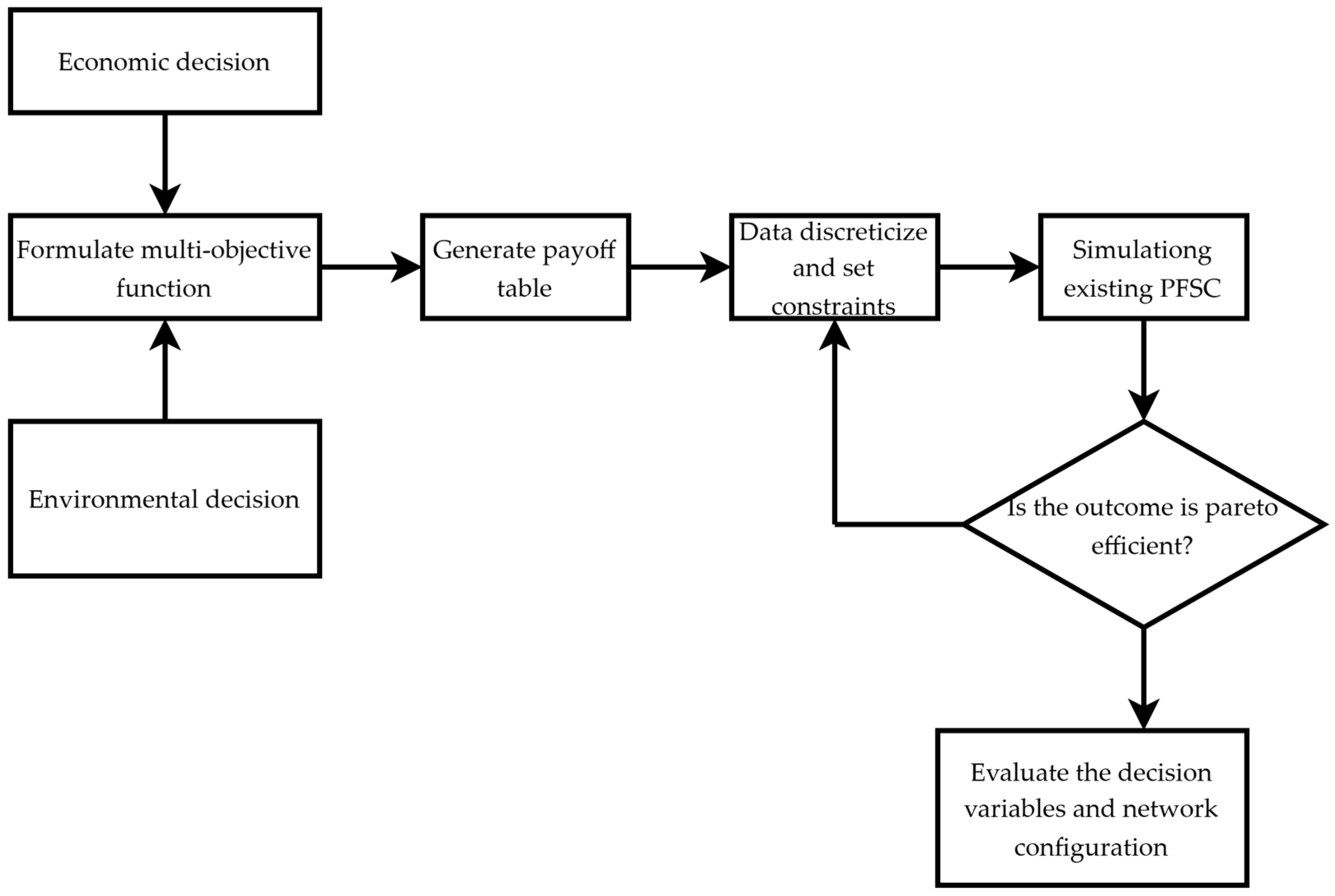
3. Materials and Methods

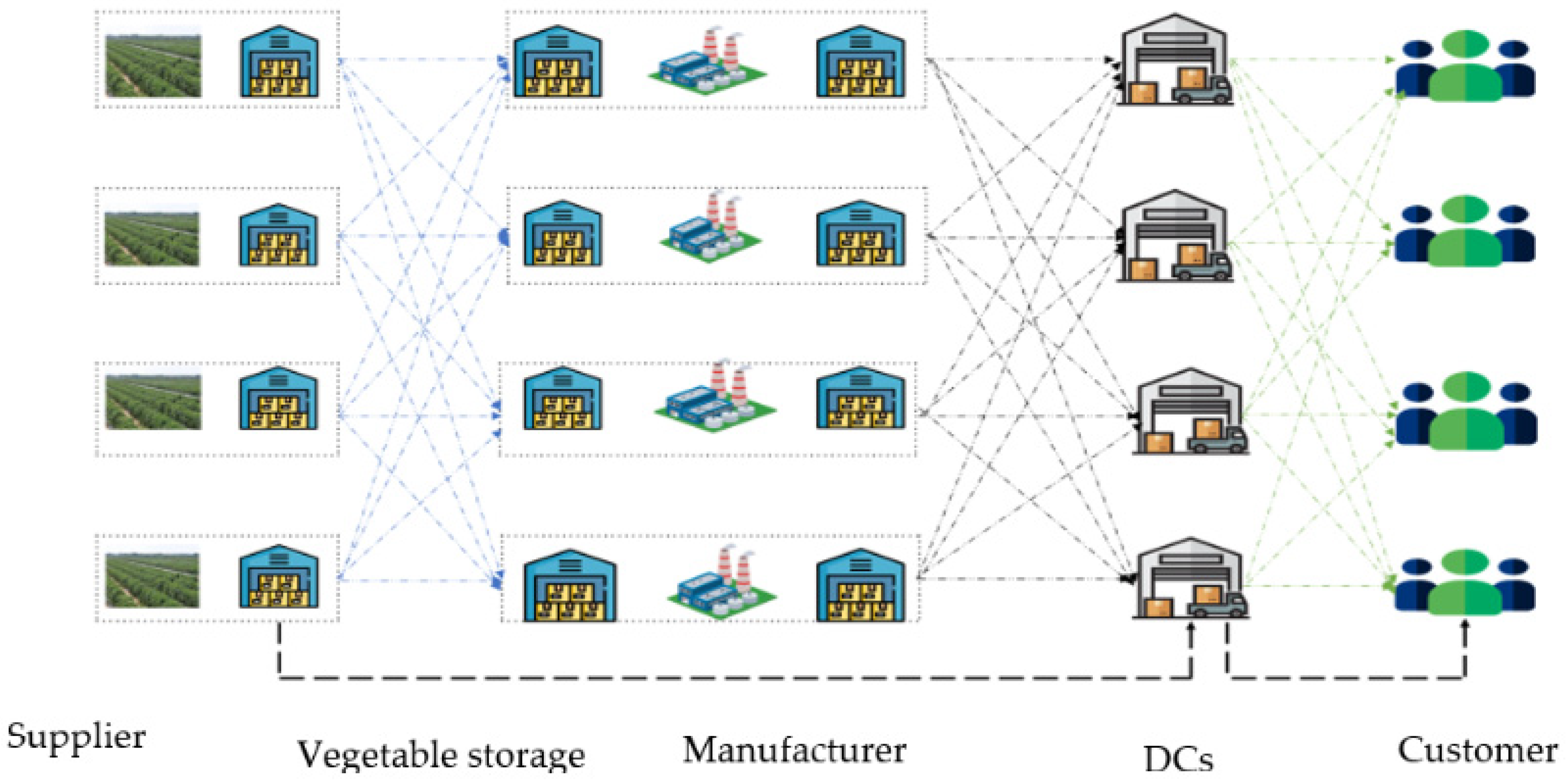
3.1. Problem Statement

As mentioned previously, this study focuses on integrated strategic and tactical decisions incorporating environmental dimension for perishable food supply chains to obtain optimal value considering a multi-supplier. For this purpose, we consider a perishable food supply chain network including supplier centers, manufacturing center, distribution centers, and customers (Figure 1), along with the interconnections between them. Through this supply network, vegetables sourced from supplier locations are transported to storage facilities and subsequently divided into two distinct supply chains: fresh vegetables are packed and dispatched to distribute without processing, while the remaining portion is transported to manufacturing site warehouses for further processing. At the manufacturing sites, the vegetables undergo processing at location m using specific technology and capacity e to produce the final product p. These final products can either be stored at the manufacturing centers or shipped directly to distribution centers. Once at the distribution centers, products are delivered to meet customer demand.

Perishable food supply chains often face uncertainties due to product characteristics, seasonality, and fluctuating consumer demand. Environmental models are used to incorporate eco-costs related to production, construction, and transportation. It is valuable to integrate a total cost (TC) and environmental impact (EI) and examine its impact on the optimal solution, considering the trade-off between cost and environmental impact.

In this paper, we intend to determine optimal network configuration to the existing infrastructure related to distance between each echelon, the time window, optimal inventory levels according to the product longevity, and allocation of resources to each echelon. The major objective of this research is finding the optimal solution for multi-objective optimization. To implement an environmental dimension like the eco-cost of construction, production and transportation must be considered as an input parameter of the model.

3.2. Model Formulation

As mentioned before, the problem results in a mixed-integer linear programming (MILP) model aimed at minimizing the total cost of the AFFSC. The proposed model encompasses a multi-product, multi-echelon, multi-inventory, and multi-period supply chain, incorporating the environmental dimension.

The design of the supply chain network also carefully addresses constraints and uncertainties that could impact the perishability characteristics of the products. Consequently, the decision variables include the location and processing capacity for each potential site, the quantity of raw materials sourced from suppliers, the amount of product produced at each location, and the inventory levels at each storage facility. These decision variables must adhere to specific constraints, including vegetable availability and mass balances at each stage, applicable to both fresh vegetables and the final products. The integrated model’s indices, parameters, and decision variables are detailed in

Table 1. Model nomenclature.

Index Sets
S	Suppliers; indexed by s Є S
M	Manufacturing centers; indexed by m Є M
D	Distribution centers; indexed by d Є D
K	Customers; indexed by k Є K
V	Vegetables; indexed by v Є V
P	Final products; indexed by $p \mathsf{Є} P$
N	Intervals in the discount schedule; indexed by n Є N
A	Distribution center capacity; indexed by a Є A
E	Manufacturing center capacity; indexed by e Є E
T	Set time periods; index t Є T
Technical Parameters
${\mu }_v$	Deterioration rate of vegetable v, %
${Yvs}_{vst}$	Available amount of vegetable v at supplier s during period t, for processing, ton
${Y2vs}_{vst}$	Available amount of vegetable v at supplier s during period t, for distribution, ton
${\beta }_{vp}$	Conversion factor of vegetable v to product p, ton of product/ton of vegetable
BC_LB1smv	Lower bound for the quantity of vegetable v shipped from supplier s to manufacturing center m to ensure business continuity in multi-sourcing strategy, ton
BC_UB1smv	Upper bound for the quantity of vegetable v shipped from supplier s to manufacturing center m to ensure business continuity in multi-sourcing strategy, ton
BC_LB2mdp	Lower bound for the quantity of product v shipped from manufacturing center m to distribution center d to ensure business continuity in multi-sourcing strategy, ton
BC_UB2mdp	Upper bound for the quantity of vegetable v shipped manufacturing center m to distribution center d to ensure business continuity in multi-sourcing strategy, ton
BC_LB3dkp	Lower bound for the quantity of product p shipped from distribution center d to customer k to ensure business continuity in multi-sourcing strategy, ton
BC_UB3dkp	Upper bound for the quantity of product p shipped from distribution center d to customer k to ensure business continuity in multi-sourcing strategy, ton
BC_LB4sdv	Lower bound for the quantity of vegetable v shipped from supplier s to distribution center m to ensure business continuity in multi-sourcing strategy, ton
BC_UB4sdv	Upper bound for the quantity of vegetable v shipped from supplier s to distribution center d to ensure business continuity in multi-sourcing strategy, ton
BC_LB5dkv	Lower bound for the quantity of vegetable v shipped from distribution center d to customer k to ensure business continuity in multi-sourcing strategy, ton
BC_UB5dkv	Upper bound for the quantity of vegetable v shipped from distribution center d to customer k to ensure business continuity in multi-sourcing strategy, ton
${Depk}_{kpt}$	Product p demand at customer k during period t, ton
${Devk}_{vkt}$	Vegetable v demand by customer k during period t, ton
${cs}_{vs}$	Capacity of supplier s in supplying vegetable v per period t
${cmp}_{me}$	Capacity to process product p at manufacturing center m with capacity e, ton
${cdp}_{da}$	Storage capacity of product p at distribution center d with capacity a, ton
$L_{vns}$	Lower bound of interval n of discount schedule that is offered by supplier s for vegetable v, ton
${Lmin}_{vm}$	Lower bound for the safety stock for vegetable v at manufacturing center m, ton
$U_{vns}$	Upper bound of interval n of discount schedule that is offered by supplier s for vegetable v, ton
M	Big M, a sufficiently large number
${\lambda }_1$	Weight of the long-term costs
${\lambda }_2$	Weight of the mid-term costs
Economic parameters
${chs}_{vs}$	Holding cost for vegetable v at supplier s for a period t, $/ton
${chm}_{vm}$	Holding cost for vegetable v at manufacturer m for a period t, $/ton
${chm}_{pm}$	Holding cost for product p at manufacturer m for a period t, $/ton
${chd}_{pd}$	Holding cost for product p at distribution center d for a period t, $/ton
${chd}_{vd}$	Holding cost for vegetable v at distribution center d for a period t, $/ton
${mc}_{pm}$	Unit manufacturing cost of product p in manufacturing center m, $/ton
${oc}_{d,a}$	Periodic operating cost for distribution center d with capacity level a, $
${pc}_{vsn}$	Unit price of vegetable v within interval n of discount schedule that is offered by supplier s, $/ton
$T_{vsm}$	Transportation distance for vegetable v from supplier s to manufacturer m, Km
$T_{pmd}$	Transportation distance for product p from manufacturer m to distribution center d, Km
$T_{pdk}$	Transportation distance for product p from distribution center d to customer k, Km
$T_{vsd}$	Transportation distance for vegetable v from supplier s to distribution center d, Km
$T_{vdk}$	Transportation distance for vegetable v from distribution center d to customer k, Km
$p_{pk}$	Sales price for product p in customer k, $/ton
${cu}_p$	Unit transportation cost of product p, $/ton Km
${cu}_v$	Unit transportation cost of vegetable v, $/ton Km
${cf}_{me}$	Investment cost for opening manufacturing center m with capacity e, $
${cf}_{da}$	Investment cost for opening distribution center d with capacity a, $
Eco cost parameters
${ECCvw}_{me}$	Production eco-costs for manufacturing center m with capacity e
${ECDC}_{da}$	Utilization eco-costs for distribution center d with capacity a
${ECTv}_{vsm}$	Transport eco-costs for vegetable v from supplier s to manufacturing center m
${ECTp}_{pmd}$	Transport eco-costs for product p from manufacturing center m to distribution center
${ECTp}_{pdk}$	Transport eco-costs for product p from distribution center d to customer k
${ECTv}_{vsd}$	Transport eco-costs for vegetable v from supplier s to distribution center d
${ECTp}_{vdk}$	Transport eco-costs for vegetable v from distribution center d to customer k
Decision variables
${U1}_{m,e}$	Binary variable with value 1 when manufacturing center with capacity level e is established at location m; 0 otherwise
${U2}_{d,a}$	Binary variable with value 1 when distribution center with capacity level a is established at location d; 0 otherwise
${X1}_{smvt}$	Binary variable with value 1 when manufacturing center m is supplied by supplier s for vegetable v in period t; 0 otherwise
${X2}_{mdpt}$	Binary variable with value 1 when distribution center d is supplied by manufacturing center m for product p in period t; 0 otherwise
${X3}_{dkpt}$	Binary variable with value 1 when customer k is supplied by distribution center d for product p in period t; 0 otherwise
$Y_{smvnt}$	Binary variable with value 1 when order quantity of manufacturing center m for vegetable v falls within interval n of the discount schedule of supplier s in time period t; 0 otherwise
${Gvs}_{vst}$	Amount of vegetable v obtained from supplier during period t, ton
${Wvm}_{vmt}$	Amount of vegetable v transformed to product at manufacturing center m during time period t, ton
${Wpm}_{pmt}$	Amount of product p produced from vegetable at manufacturing center m during time period t, ton
${ISvs}_{vst}$	Inventory level at supplier center s of vegetable v at the end of period t, ton
${IMvm}_{vmt}$	Inventory level at manufacturing center m of vegetable v at the end of period t, ton
${IMpm}_{pmt}$	Inventory level at manufacturing center m of product p at the end of period t, ton
${IDpd}_{pdt}$	Inventory level at distribution center d of product p at the end of period t, ton
${IDvd}_{vdt}$	Inventory level at distribution center d of vegetable v at the end of period t, ton
${WY}_{smvnt}$	Quantity of order for vegetable v that is released from manufacturing center m to supplier s within discount schedule n in the time period t, ton
${W1}_{smvt}$	Quantity of order for vegetable v that is released from manufacturing center m to supplier s in the time period t, ton
${W2}_{mdpt}$	Quantity of order for product p that is released from distribution center d to manufacturing center m in the time period t, ton
${W3}_{dkpt}$	A fraction of order for product p by customer k that can be satisfied by distribution center d in the time period t, ton
${W4}_{sdvt}$	Quantity of vegetable v supplied from supplier s to distribution center d in the time period t, ton
${W5}_{dkvt}$	Quantity of vegetable v supplied from distribution center d customer k during the time period t, ton

.

The problem is formulated as a mixed-integer linear programming (MILP) model with a dual objective of minimizing both total costs and environmental impacts. It captures a multi-product, multi-echelon, multi-inventory, multi-period supply chain and explicitly incorporates environmental considerations. To account for product perishability, the network design integrates relevant constraints and uncertainties throughout the chain. Key decision variables determine which sites to open and their processing capacities, how much raw material to order from each supplier, the production levels at each facility, and inventory holdings at each storage location. All decisions must satisfy constraints on vegetable availability and mass balance at every stage for fresh inputs as well as final outputs. A complete list of indices, parameters, and decision variables is presented in Table 1.

The lines in Figure 1 represent the network connections at each stage of the perishable food supply chain. Specifically, this model superstructure outlines two distinct product supply chains. The first supply chain, represented by the upper lines, illustrates the network involving suppliers, manufacturing centers, distribution centers, and customers, specifically for tomatoes intended for processing. The second supply chain, indicated by the lower lines, details the distribution of tomatoes that are not processed. This flow starts from suppliers to distribution centers and then moves to customers.

3.3. Model Constraints

3.3.1. Production and Harvest Constraint

Constraint (1) guarantees that the total quantity of vegetable v sourced from supplier s during time period t does not exceed its available supply.

$${Gvs}_{vst}\le {Yvs}_{vst} ⩝s Є S, tЄT, ⩝v Є V$$

(1)

Constraint (2) defines the uniqueness constraints, where (2a) applies to the establishment of a manufacturing center with capacity e at location m and (2b) applies to the establishment of a distribution center with capacity a at location d.

$$\sum _{eЄE}{U1}_{me} \le 1 ; ⩝m Є M$$

(2a)

$$\sum _{aЄA}{U2}_{da} \le 1 ; ⩝d Є D$$

(2b)

3.3.2. Multi-Sourcing Strategy

In the multi-sourcing strategy, we can impose a lower bound and an upper bound between a buyer and a supplier to ensure a lasting relationship and eventually establish a quantity discount strategy (respectively, to limit the dependence from a supplier). The constraints (3) to (7) impose these lower and upper limits, respectively, between a supplier and a manufacturing center for raw materials (3), a manufacturing center and a distribution center for products (4), from a distribution center and a client for products (5), a supplier and a distribution center for raw materials (6), and a distribution center and a client for raw materials (7):

$${ BC\text{\_}LB1}_{smv}\le {W1}_{smvt}\le {BC\text{\_}UB1}_{smv} \forall s\in S, m\in M, v\in V, t Є T$$

(3)

$${BC\text{\_}LB2}_{mdp}\le {W2}_{mdpt}\le {BC\text{\_}UB2}_{mdp} \forall m\in M, d\in D, p\in P, t Є T$$

(4)

$${BC\text{\_}LB3}_{dkp}\le {W3}_{dkpt}\le {BC\text{\_}UB3}_{dkp} \forall d\in D, k\in K, p\in P, t Є T$$

(5)

$${BC\text{\_}LB4}_{sdv}\le {W4}_{sdvt}\le {BC\text{\_}UB4}_{sdv} \forall s\in S, d\in D, v\in V, t Є T$$

(6)

$${BC\text{\_}LB5}_{dkv}\le {W5}_{dkvvt}\le {BC\text{\_}UB5}_{dkv} \forall d\in D, k\in K, v\in V, t Є T$$

(7)

3.3.3. Capacity Constraints

Constraint (8) guarantees that the quantity of vegetable v supplied by supplier s to all manufacturing centers during period t remains within its shipping capacity limit.

$$\sum _{mЄ M}{W1}_{smvt} \le {cs}_{vs} ; s Є S, v Є V, t Є T$$

(8)

Constraint (9) stipulates that, for each supplier s, the total amount of vegetable v delivered to all distribution centers during period t must not exceed the allocated quantity for the distribution centers.

$$\sum _{dЄ D}{W4}_{sdvt} \le {Y2vs}_{vst} ; ⩝s Є S, v Є V, t Є T$$

(9)

Constraint (10) sets the upper limit for production capacity. It ensures that the total amount of product p produced at each manufacturing center during time period t does not exceed the manufacturing center’s capacity.

$$\sum _{p Є P}{Wpm}_{pmt}\le \sum _{eЄ E}{{cmp}_{me}\ast U1}_{me} ; ⩝m Є M, t Є T$$

(10)

Constraint (11) applies the same limitation for product p but in the context of storage. It ensures that the total amount of product p stored in each distribution center d during time period t does not exceed the maximum storage capacity.

$$\sum _{p Є P}{IDpd}_{pdt} \le \sum _{aЄ A}{{cdp}_{da}\ast U2}_{da} ; ⩝d Є D, t Є T$$

(11)

3.3.4. Decision Variables for Allocation and Order Quantities

An order for each vegetable v is issued from manufacturing center m to supplier s only if the supplier exists and is active.

$${W1}_{smvt}\le {M X1}_{smvt } ; ⩝s Є S, m Є M, v Є V, t Є T$$

(12)

An order for each product p is placed from distribution center d to manufacturing center m only if the manufacturing center exists and is active.

$${W2}_{mdpt }\le {M X2}_{mdpt ; }⩝m Є M, d Є D, p Є P, tЄ T$$

(13)

An order for each product p is placed from customer k to distribution center d only if the distribution center exists and is active.

$${W3}_{dkpt }\le {M X3}_{dkpt } ; ⩝d Є D, k Є K, p Є P, t Є T$$

(14)

3.3.5. Constraints on the Discount Rate

The adoption of a pricing policy predicated on quantity discounts necessitates a purchase price for raw materials that is contingent upon the quantity demanded. In practical terms, this entails partitioning the entire range of raw material quantities to be supplied into discrete sub-intervals, each characterized by a constant, progressively decreasing price as the demanded volume increases. From a modeling perspective, the price is represented as a piecewise constant function that varies in relation to the quantity. Accordingly, for each time period t, each vegetable v, and each order placed between a supplier s and a manufacturing center m, it becomes imperative to identify the specific quantity interval to be selected through the binary decision variable $Y_{smvnt}$. Thus, the quantity dispatched by the supplier must reside within the lower and upper bounds of the chosen interval, as delineated by Equations (15) and (16).

$${W1}_{smvt }\ge \sum _{nЄN}{L}_{vns}{Y}_{smvnt} ; ⩝s Є S, m Є M, v Є V, t Є T$$

(15)

$${W1}_{smvt}\le \sum _{nЄN}{U}_{vns}{Y}_{smvnt} ; ⩝s Є S, m Є M, v Є V, t Є T$$

(16)

Furthermore, if a flow of vegetables v occurs between supplier s and manufacturing center m during period t, it is imperative to select the sub-interval corresponding to the quantity to be dispatched. This condition is represented by Equation (17).

$$\sum _{nЄN}{Y}_{smvnt}={X1}_{smvt} ; ⩝s Є S, m Є M, v Є V, tЄ T$$

(17)

3.3.6. Material Balance Constraints

For each supplier s and vegetable v, the inventory level at the end of period t is the inventory level from the previous period, adjusted for vegetable deterioration (${\mu }_v$), plus the quantity received by the supplier, minus the quantity delivered to the network (to all manufacturing centers).

$${{ISvs}_{vst}=\left(1-{\mu }_V\right)\ast ISvs}_{vs\left(t-1\right)}+{Gvs}_{v,s,t}-\sum _{mЄM}{W1}_{smvt} ⩝vЄV,sЄS,tЄT$$

(18)

In a similar manner, at each manufacturing center m, for a vegetable v, the inventory level at the end of period t is determined by the inventory level from the preceding period, considering vegetable deterioration (${\mu }_v$), plus the quantity received from all suppliers, and minus the quantity of vegetable transformed into the final product.

$${IMvm}_{vmt}=\left(1-{\mu }_V\right)\ast {IMvm}_{vm\left(t-1\right)}+\sum _{sЄS}{W1}_{smvt}-{Wvm}_{vmt} ⩝vЄV,tЄT,mЄM$$

(19)

At each manufacturing center m, a safety stock may be designated (or not if ${Lmin}_{vm}=0$) for each vegetable v during time period t.

$${IMvm}_{vmt}\ge {Lmin}_{vm} ⩝vЄV,tЄT,mЄM$$

(20)

Constraint (21) determines the quantity of product p produced through the transformation of vegetable v at manufacturing center m (${\beta }_{vp}$ represents the transformation rate from vegetable v to product p). This transformation rate is influenced by the age of the stored raw material, with the rate decreasing as the vegetable is stored for longer periods.

$${ Wpm}_{pmt}={\beta }_{vp} {Wvm}_{vmt} ⩝vЄV,mЄM,tЄT,pЄP$$

(21)

At each manufacturing center, constraint (22) is analogous to Equation (19) but applied to the product. The primary difference is that the product does not experience degradation. The inventory level of product p at the end of period t is equal to the inventory from the previous period, plus the quantity produced, minus the total amount of product dispatched to the distribution centers d.

$${{IMpm}_{pmt}=IMpm}_{pm\left(t-1\right)}+{Wpm}_{pmt}-\sum _{dЄD}{W2}_{mdpt} ⩝mЄM,pЄP,tЄT$$

(22)

Constraint (23) is similar to constraint (22) but applies at each distribution center. It accounts for the stock of product p at distribution center d, the quantity received from all manufacturing centers, and the quantity shipped to all clients k.

$${{IDpd}_{pdt}=IDpd}_{pd\left(t-1\right)}+\sum _{mЄM}{W2}_{mdpt}-\sum _{kЄK}{W3}_{dkpt} ⩝dЄD,pЄP,tЄT$$

(23)

Since vegetables can be sent directly to the distribution centers, a mass balance for vegetables must also be enforced. Given that vegetables are subject to deterioration, this must be taken into account. Therefore, Equation (24) is analogous to constraint (19) but applied at each distribution center.

$${IDvd}_{vdt}=\left(1-{\mu }_V\right)\ast {IDvd}_{vd\left(t-1\right)}+\sum _{sЄS}{W4}_{sdvt}-\sum _{k\in K}{W5}_{dkvt} ⩝vЄV,tЄT,dЄD$$

(24)

3.3.7. Satisfaction of Demand Requirements

The quantity of product transported from distribution center d to customer k in each time period t is equal to the amount of product p requested by customer k, as specified by constraint (25).

$$\sum _{dЄD}{W3}_{dkpt}={Depk}_{kpt} ⩝pЄP,tЄT,kЄK$$

(25)

Constraint (26) is identical to the previous one but applies to the demand for fresh vegetable v.

$$\sum _{dЄD}{W5}_{dkvt}={Devk}_{vkt} ⩝vЄV,tЄT,kЄK$$

(26)

3.3.8. Constraint for Initialization

Due to time discretization, initial conditions are essential, such as the initial levels of products or raw materials. The initialization values depend on the specific context of the supply chain, and in our case study, they are set to 0.

$${ISvs}_{v,s,0=}0, { IMvm}_{v,m,0}=0, { IMpm}_{p,m,0}=0, { IDpd}_{p,d,0}=0 ⩝mЄM,dЄD,vЄV,sЄS,p⩝P$$

(27)

3.3.9. Constraints on Non-Negativity

$$\begin{gathered} { ISvs}_{vst}, {IMvm}_{vmt},{IMpm}_{pmt},{IDpd}_{pdt},{W1}_{smvt},{W2}_{mdpt},{W3}_{dkpt}\ge 0 \\ ⩝vЄV,mЄM,dЄD,kЄK,sЄS,tЄT,pЄP \end{gathered}$$

(28)

3.4. Objective Function

Min f = Raw Material Purchase + Investment Cost + Production Cost + Operating Cost + Inventory Holding Cost +Transportation Cost

$$\mathbf{R}\mathbf{a}\mathbf{w} \mathbf{M}\mathbf{a}\mathbf{t}\mathbf{e}\mathbf{r}\mathbf{i}\mathbf{a}\mathbf{l} \mathbf{P}\mathbf{u}\mathbf{r}\mathbf{c}\mathbf{h}\mathbf{a}\mathbf{s}\mathbf{e}=\sum _{vЄV}\sum _{sЄS}\sum _{nЄN}\sum _{mЄM}\sum _{tЄT}{pc}_{vsn}\ast W_{smvt}{Y}_{smvnt}$$

(29a)

This component of the objective function is nonlinear because of the term ${ W}_{smvt}{Y}_{smvnt}$. However, it can be linearized by expressing it in the following form and incorporating constraints (30) to (32) into the initial model, utilizing the variable ${WY}_{smvnt}$.

$$\mathbf{R}\mathbf{a}\mathbf{w} \mathbf{M}\mathbf{a}\mathbf{t}\mathbf{e}\mathbf{r}\mathbf{i}\mathbf{a}\mathbf{l} \mathbf{P}\mathbf{u}\mathbf{r}\mathbf{c}\mathbf{h}\mathbf{a}\mathbf{s}\mathbf{e}=\sum _{vЄV}\sum _{sЄS}\sum _{nЄN}\sum _{mЄM}\sum _{tЄT}{pc}_{vsn}\ast {WY}_{smvnt}$$

(29b)

$${WY}_{smvnt}\le M\ast Y_{smvnt} ⩝sЄS,mЄM,vЄV, nЄN,tЄT$$

(30)

$${ WY}_{smvnt}\le {W1}_{smvt} ⩝sЄS,mЄM,vЄV, nЄ N,tЄT$$

(31)

$${ WY}_{smvnt}\ge {W1}_{smvt}-M\ast \left(1-Y_{smvnt}\right) ⩝sЄS,mЄM,v Є V, n ЄN,tЄ T$$

(32)

$$\mathbf{I}\mathbf{n}\mathbf{v}\mathbf{e}\mathbf{s}\mathbf{t}\mathbf{m}\mathbf{e}\mathbf{n}\mathbf{t} \mathbf{C}\mathbf{o}\mathbf{s}\mathbf{t}={\lambda }_1\left(\sum _{mЄM}\sum _{eЄE}{cf}_{me}\ast {U1}_{me}+\sum _{dЄD}\sum _{aЄA}{cf}_{da}\ast {U2}_{da}\right)$$

(33)

$$\mathbf{P}\mathbf{r}\mathbf{o}\mathbf{d}\mathbf{u}\mathbf{c}\mathbf{t}\mathbf{i}\mathbf{o}\mathbf{n} \mathbf{C}\mathbf{o}\mathbf{s}\mathbf{t}=\sum _{pЄP}\sum _{mЄM}\sum _{dЄD}\sum _{tЄT}{mc}_{pm}\ast W_{mdpt}$$

(34)

$$\mathbf{O}\mathbf{p}\mathbf{e}\mathbf{r}\mathbf{a}\mathbf{t}\mathbf{i}\mathbf{n}\mathbf{g} \mathbf{C}\mathbf{o}\mathbf{s}\mathbf{t}\mathbf{a}\mathbf{t} \mathbf{D}\mathbf{i}\mathbf{s}\mathbf{t}\mathbf{r}\mathbf{i}\mathbf{b}\mathbf{u}\mathbf{t}\mathbf{i}\mathbf{o}\mathbf{n} \mathbf{C}\mathbf{e}\mathbf{n}\mathbf{t}\mathbf{e}\mathbf{r}={\lambda }_2\sum _{dЄD}\sum _{aЄA}\sum _{mЄM}\sum _{pЄP}\sum _{tЄT}{oc}_{d,a}\ast W_{mdpt}$$

(35)

$$\begin{array}{l}\mathbf{Inventory holding cost}\\ ={\displaystyle \sum _{vЄV}}{\displaystyle \sum _{sЄS}}{\displaystyle \sum _{tЄT}}{{chs}_{vs}\ast ISvs}_{vst}+{\displaystyle \sum _{vЄV}}{\displaystyle \sum _{mЄM}}{\displaystyle \sum _{tЄT}}{{chm}_{vm}\ast IMvm}_{vmt}+{\displaystyle \sum _{pЄP}}{\displaystyle \sum _{mЄM}}{\displaystyle \sum _{tЄT}}{{chm}_{pm}\ast IMpm}_{pmt}\\ +{\displaystyle \sum _{pЄP}}{\displaystyle \sum _{dЄD}}{\displaystyle \sum _{tЄT}}{{chd}_{pd}\ast IDpd}_{pdt}+{\displaystyle \sum _{vЄV}}{\displaystyle \sum _{dЄD}}{\displaystyle \sum _{tЄT}}{{chd}_{vd}\ast IDvd}_{dvt} \end{array}$$

(36)

$$\begin{array}{l}\mathbf{Transportation cost}\\ ={\displaystyle \sum _{vЄV}}{\displaystyle \sum _{sЄS}}{\displaystyle \sum _{mЄM}}{\displaystyle \sum _{tЄT}}{{cu}_v\ast T}_{vsm}\ast {W1}_{smvt}\\ +{\displaystyle \sum _{pЄP}}{\displaystyle \sum _{mЄM}}{\displaystyle \sum _{dЄD}}{\displaystyle \sum _{tЄT}}{{cu}_p\ast T}_{pmd}\ast {W2}_{mdpt}+{\displaystyle \sum _{pЄP}}{\displaystyle \sum _{dЄD}}{\displaystyle \sum _{kЄK}}{\displaystyle \sum _{tЄT}}{{cu}_p\ast T}_{pdk}\ast {W3}_{dkpt}\\ +{\displaystyle \sum _{vЄV}}{\displaystyle \sum _{sЄS}}{\displaystyle \sum _{dЄD}}{\displaystyle \sum _{tЄT}}{{cu}_V\ast T}_{vsd}\ast {W4}_{sdvt}+{\displaystyle \sum _{vЄV}}{\displaystyle \sum _{kЄK}}{\displaystyle \sum _{dЄD}}{\displaystyle \sum _{tЄT}}{{cu}_V\ast T}_{vsk}\ast {W5}_{dkvt} \end{array}$$

(37)

Min Eco-costs = Ecocost Production + Ecocost Construction + Ecocost Transport Cost

$$\mathbf{E}\mathbf{c}\mathbf{o}\mathbf{c}\mathbf{o}\mathbf{s}\mathbf{t} \mathbf{P}\mathbf{r}\mathbf{o}\mathbf{d}\mathbf{u}\mathbf{c}\mathbf{t}\mathbf{i}\mathbf{o}\mathbf{n}=\sum _{v\in V}\sum _{m\in M}\sum _{t\in T}\left(rate\ast \left({Wvm}_{vmt}\right)\right)$$

(38)

$$\mathbf{E}\mathbf{c}\mathbf{o}\mathbf{c}\mathbf{o}\mathbf{s}\mathbf{t} \mathbf{C}\mathbf{o}\mathbf{n}\mathbf{s}\mathbf{t}\mathbf{r}\mathbf{u}\mathbf{c}\mathbf{t}\mathbf{i}\mathbf{o}\mathbf{n}=\sum _{m\in M}\sum _{e\in E}\sum _{t\in T}\left({ECCv}_{me}\ast \left({U1}_{met}-{U1}_{m,e,t-1}\right)\right)+\sum _{d\in D}\sum _{a\in A}\sum _{t\in T}\left({ECDC}_{da}\ast \left({U2}_{dat}-{U2}_{d,a,t-1}\right)\right)$$

(39)

$$\begin{array}{l}\mathbf{E}\mathbf{c}\mathbf{o}\mathbf{c}\mathbf{o}\mathbf{s}\mathbf{t} \mathbf{T}\mathbf{r}\mathbf{a}\mathbf{n}\mathbf{s}\mathbf{p}\mathbf{o}\mathbf{r}\mathbf{t} \mathbf{C}\mathbf{o}\mathbf{s}\mathbf{t}\\ ={\displaystyle \sum _{v\in V}}{\displaystyle \sum _{s\in S}}{\displaystyle \sum _{m\in M}}{\displaystyle \sum _{t\in T}}\left({ECTv}_{vsm}\ast W_{smvt}\right)\\ +{\displaystyle \sum _{p\in P}}{\displaystyle \sum _{m\in M}}{\displaystyle \sum _{d\in D}}{\displaystyle \sum _{t\in T}}\left({ECTP}_{pmd}\ast W_{mdpt}\right)\\ +{\displaystyle \sum _{p\in P}}{\displaystyle \sum _{d\in D}}{\displaystyle \sum _{k\in K}}{\displaystyle \sum _{t\in T}}\left({ECTp}_{pdk}\ast W_{dkpt}\right)\\ +{\displaystyle \sum _{v\in V}}{\displaystyle \sum _{s\in S}}{\displaystyle \sum _{d\in D}}{\displaystyle \sum _{t\in T}}\left({ECTV}_{vsd}\ast W_{sdvt}\right)\\ +{\displaystyle \sum _{v\in V}}{\displaystyle \sum _{d\in D}}{\displaystyle \sum _{k\in K}}{\displaystyle \sum _{t\in T}}\left({ECTv}_{vdk}\ast W_{dkvt}\right) \end{array}$$

(40)

To evaluate the environmental impact of the perishable food supply chain, the life cycle assessment (LCA) approach is applied. This ISO-standardized tool is widely used to assess the environmental footprint of supply chains, particularly for perishable food products that have high resource dependency and short shelf life [34,35]. The LCA consists of three key steps: goal and scope definition, life cycle inventory (LCI), and impact assessment [34]. In the goal and scope definition phase, the system boundaries and functional unit are established. Given the high perishability of tomatoes, the supply chain boundaries range from the vegetable supplier’s gate to the final tomato paste product, encompassing all processing, storage, and transportation activities (see Figure 1). The functional unit chosen for this study is one metric ton (MT) of tomato paste, ensuring that environmental impacts are measured on a standardized basis. The data for this assessment are sourced from [36]. The second step, life cycle inventory (LCI), involves identifying and quantifying the raw material inputs, energy consumption, emissions, and waste generated throughout the product’s life cycle [34]. Given the time-sensitive nature of perishable food supply chains, inventory analysis includes detailed tracking of energy use in cold storage, processing losses, and transportation efficiency across different supply chain stages. In the third step, environmental impact assessment, the eco-costs method introduced by [37] and more recently by [38] studies process engineering supply chains and demonstrates its efficiency to quantify the environmental impact. Eco-costs measure the environmental impact of a product by evaluating the costs of preventing environmental damage throughout its life cycle. For this work, we have adopted this method because (1) it is well suited for evaluating the environmental impact of supply chain, as proven in our previous studies; (2) the final result is translated into monetary value that makes it easy to compare with the economic criteria; (3) unlike other LCAs, comparison with other products is not necessary; and (4) the cost and the system are regularly updated to take into account the recent improvement and evolutions (in this study we use the more recent version, i.e., 2022).

By integrating LCA with eco-cost analysis, this study provides a comprehensive evaluation of the environmental trade-offs in perishable food supply chains, helping optimize sustainable practices in tomato paste production and distribution.

4. Case Study

Ethiopia, with its diverse climate zones and rapidly growing economy, stands as one of Africa’s most agriculturally significant countries. Its economy grew 7.1% in 2022/23 up from 6.4% in 2021/22, and the nation’s agricultural sector is a critical component of its economy, contributing to 32 percent of the GDP and employing 85 percent of the population. However, the management of perishable food supply chains in Ethiopia presents both unique challenges and opportunities, particularly in the context of fresh fruits, vegetables, dairy products, and meat, which require meticulous handling and timely delivery to maintain quality and safety. Despite the government’s push to transform Ethiopia into a major manufacturing hub through integrated agro-processing industrial parks, the sector suffers from slow growth due to policy neglect, fragile markets, and high investment requirements. Consequently, the country incurs an annual economic loss of approximately 1.2 billion USD, nearly 10% of its average national budget from 2018 to 2022 [39].

According to data from the Central Statistical Agency (CSA), the total area dedicated to fruits, vegetables, and root crops in Ethiopia was approximately 603,207 hectares in 2019/20. Of this, 41% was allocated to root crops, while vegetables and fruits occupied 40% and 19%, respectively. One of the significant challenges in horticultural production is the perishable nature of these crops, which poses substantial difficulties in their marketing. During peak harvest seasons, fruits and vegetables are often sold at extremely low prices due to the lack of adequate preservation and storage facilities. To extend the shelf life of post-harvest produce, processing becomes essential, as it not only allows for the availability of these products during off-seasons but also enhances their market value. This processing capability can incentivize producers to increase their production, provided there is a reliable market for their products.

To address this, the Ethiopian government must reform the agricultural fresh food supply chain by establishing more processing plants and enhancing the supply chain, which could not only meet local demand but also create export opportunities to regional, Middle Eastern, and European markets.

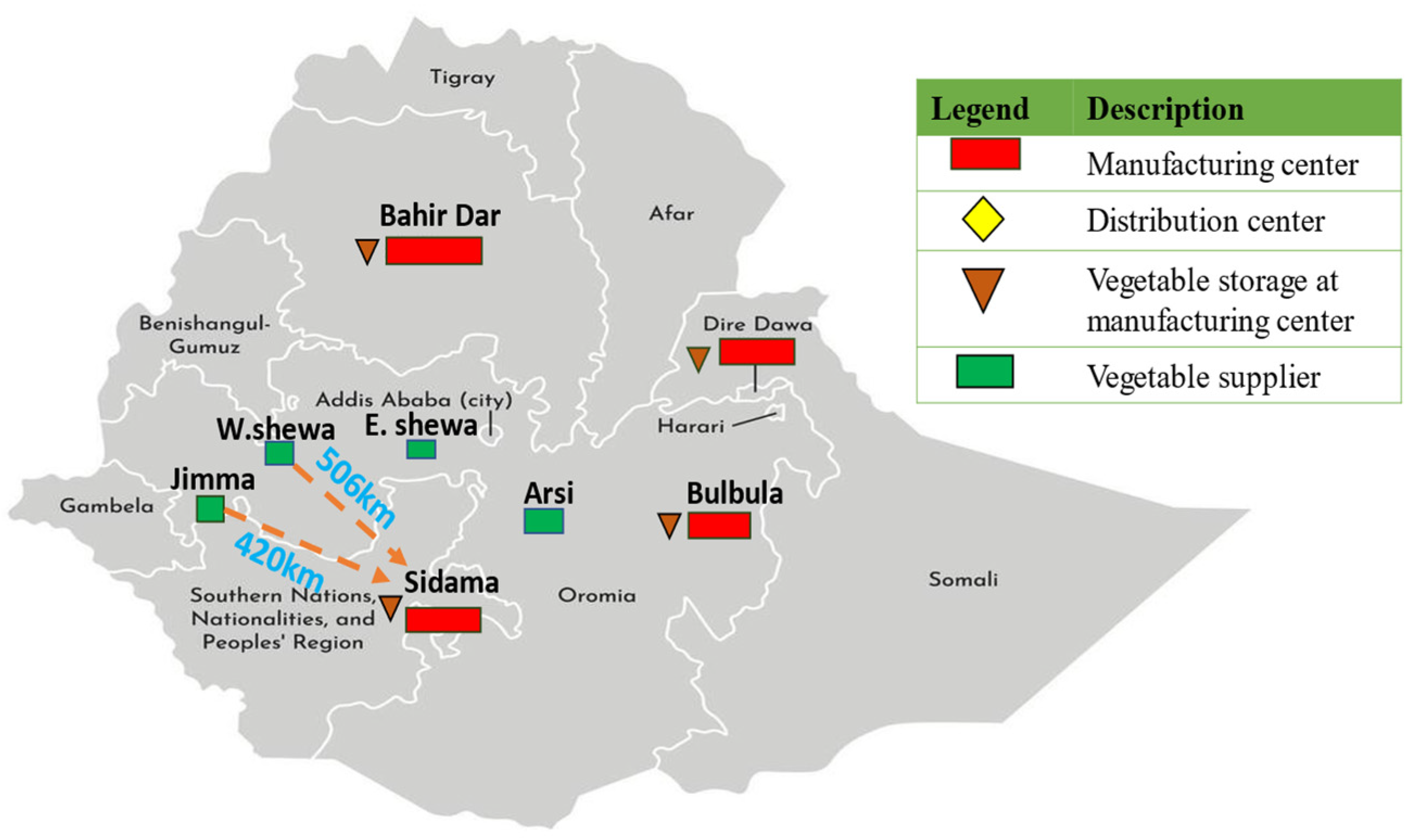
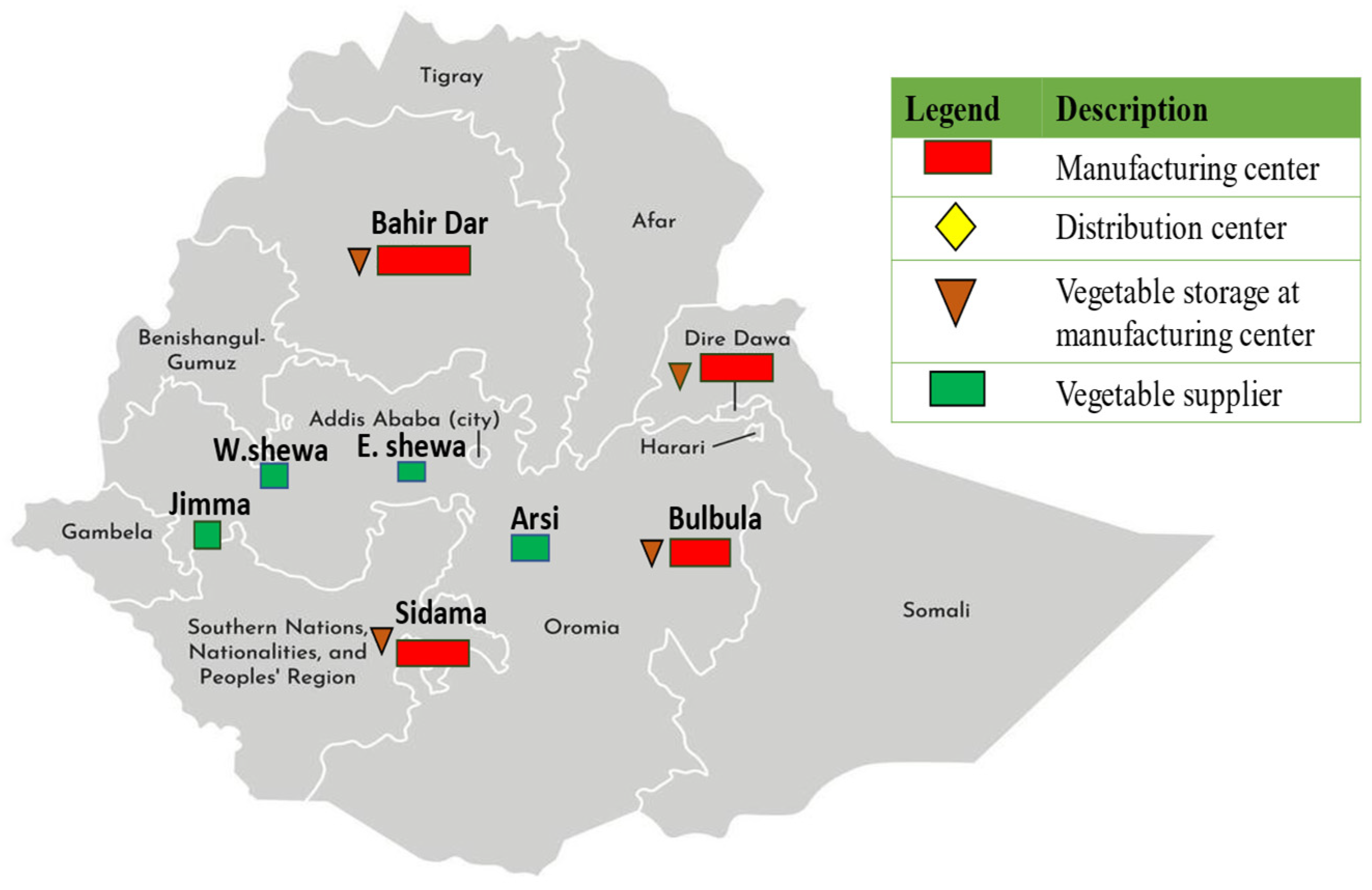
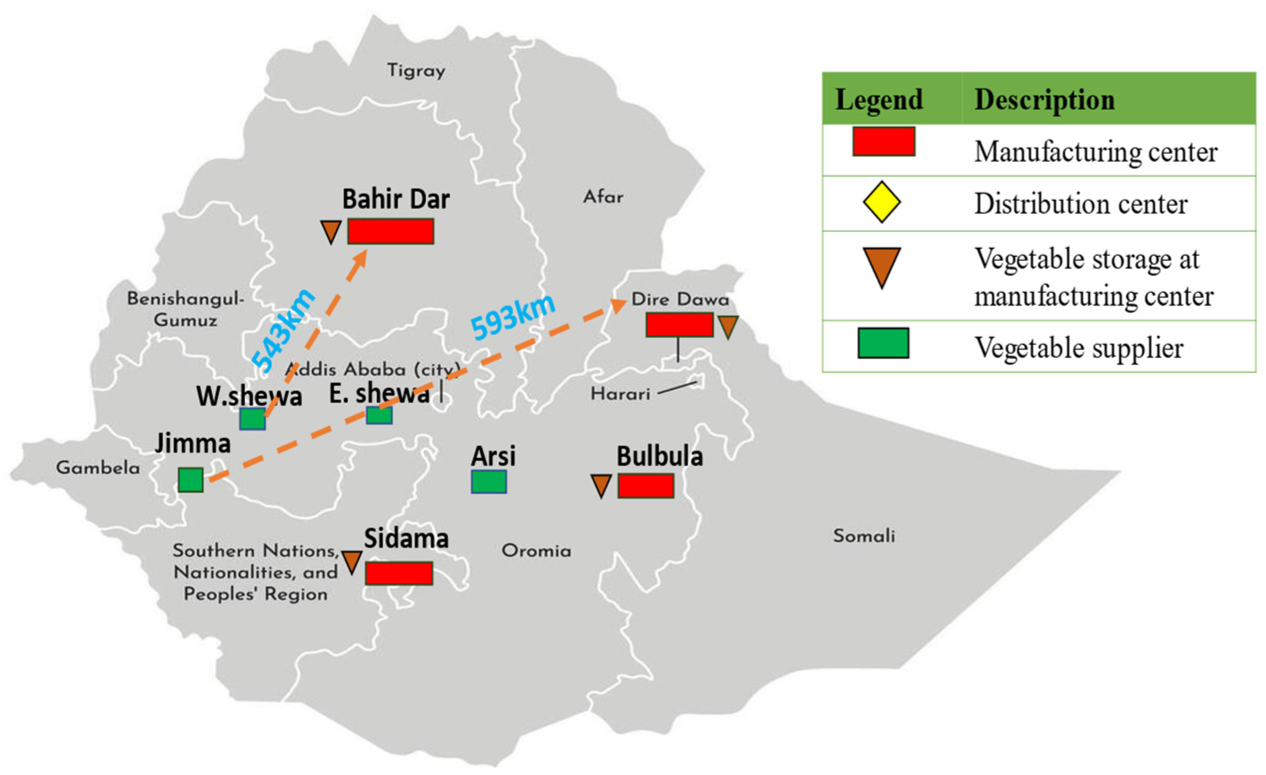
4.1. Candidate Location

To identify the key actors in Ethiopia’s agricultural food supply chain (AFFSC), the country’s administrative structure was analyzed, revealing significant disparities in land area across its nine regions and two city administrations, ranging from 0.034 million hectares in the region of Harari to 28.5 million hectares in the region of Oromia. Given its vast production potential, Oromia was chosen as the primary supplier location. This region is administratively divided into 39 zones, with tomato production occurring in only 20 of them. Among these, East Shewa, Jimma, West Shewa, and Arsi were selected as the most promising suppliers.

Since raw material suppliers are the foundational stage of the agricultural food supply chain (AFFSC), sustainable supplier selection is crucial to the overall performance of the food processing sector [32]. Potential suppliers are chosen based on their production potential and strategic positioning within production corridors, which are emerging as key hubs of rapid economic growth. Additionally, the selection process aligns with the government’s strategic direction, ensuring that the chosen suppliers contribute effectively to the sector’s development.

4.2. Demand for Tomato

To forecast tomato paste demand during the planning period, data from the Ethiopian Revenue and Customs Authority was analyzed, revealing that tomato consumption in Ethiopia is expected to reach 30,000 metric tons by 2026; this is a 2.9% increase from 25,000 metric tons in 2021. Since 2017, demand has grown by approximately 3% annually, driven by factors such as urbanization and population growth. Meanwhile, tomato production, which was 29,300 metric tons in 2021, is projected to increase at a rate of around 1% per year. The demand for tomato paste is concentrated in four urban centers: Bahir Dar, Sidama, Dire Dawa, and Bulbula are selected based on their urbanization, market potential, inter-industry linkages, infrastructure, and attractiveness to investors. Once the potential customer locations or demand areas are identified, the subsequent step involves finding, selecting, and engaging the right suppliers to meet customer needs. In this context, most of the suppliers are located in the Oromia region, and the selection process prioritizes their production capabilities.

4.3. Data

The data were sourced from various databases provided by Ethiopian government agencies, statistical institutions, and private companies operating within the country. The tomato production data (in tons) were collected from the Ethiopian Statistical Service, covering the period from 2017/18 to 2020/21 in the Oromia region. Based on these data, we forecasted production for the next ten years to capture trends and patterns relevant to our analysis. Furthermore, we focused on specific zones within Oromia that are recognized as potential areas for tomato production, ensuring that our data reflect the most pertinent regions. However, there are limitations regarding data availability, primarily due to external political factors that have affected the consistency and reliability of the data in the Oromia region. These factors may have introduced variability that could impact our findings.

Before being utilized in the model for computational experiments, the collected data underwent pretreatment to ensure consistency and homogeneity. This process involved consolidating and reconciling the data to enhance confidence in the results and validate the model’s capabilities.

After harvesting, tomatoes are typically consolidated at supply centers, a practice that simplifies supply chain management. At these centers, tomatoes undergo various treatments such as washing, grading, transformation, and packaging to ensure they meet quality and food safety standards. The packaging, tailored to market requirements, can include crates, bags, or other containers. Once packaged, the tomatoes or their processed products are distributed to various market actors, including wholesalers, retailers, and other distribution channels. Distribution can occur at local, regional, or national levels, depending on the scale of production and the demand.

East Shewa, Jimma, West Shewa, and Arsi have been identified as potential locations for fresh tomato production or as supplier locations. The yearly production data for tomatoes is sourced from the Ethiopian Statistics Service. For the manufacturing center, the upper production capacity of tomato paste was determined by considering the forecasted demand within the planning period. Meanwhile, the Merti-Agro-Processing Industry, a key tomato paste manufacturer in Ethiopia, was identified as having a lower capacity level. Based on these upper and lower bounds, six capacity levels of tomato paste processing were evaluated in this study.

The investment cost for the tomato production plant was estimated using the food process design principles outlined by [40]. The production cost of tomato paste was established based on data obtained from the existing tomato paste manufacturing industry in Ethiopia. Our categorization of capacity levels is rooted in a comprehensive analysis of projected tomato paste demand over the next ten years, which allows us to establish monthly requirements that guide our capacity planning. The six levels (0%, 20%, 35%, 50%, 70%, and 90%) were deliberately selected to represent a gradual ramp-up in production capacity. By starting at zero in the first year, we can model realistic growth trajectories for new processing plants. This incremental approach not only facilitates performance benchmarking but also adheres to best practices in capacity management, ensuring that our framework is both practical and applicable to the local context.

Once the actual investment cost for one production capacity is known, it can be estimated for the six capacity-level tomato paste manufacturing centers using Chilton’s law equation [41], with a coefficient of 0.74 for vegetables [42]. The deterioration rate of fresh tomatoes during storage was sourced from [43], and the inventory holding cost for perishable products was obtained from [44]. These costs were updated to reflect the current market conditions and the realities of the AFFSC in Ethiopia, with surveys conducted among professionals in the sector to ensure accuracy.

5. Result and Discussion

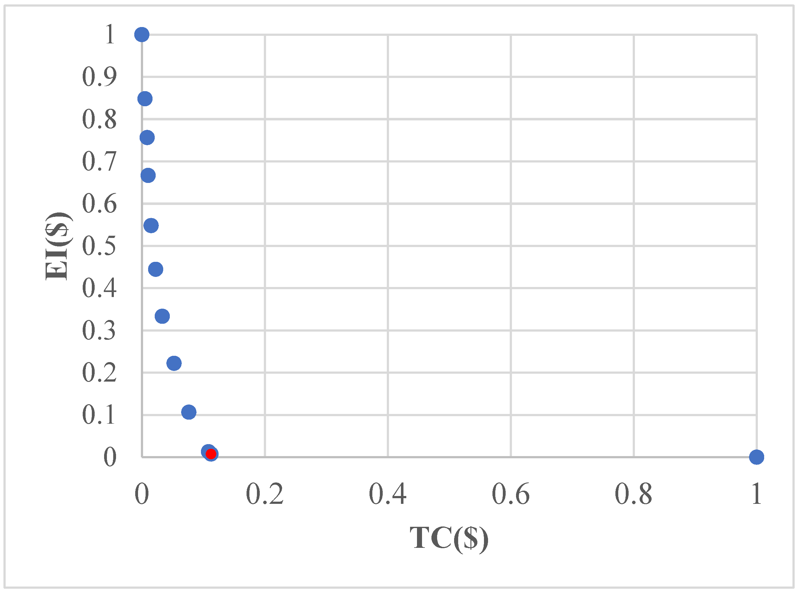
5.1. Multi-Objective Optimization Approach for Strategic and Tactical Decision Making

Before addressing the multi-objective optimization problem, it is crucial to verify whether the two objectives are antagonistic. To achieve this, separate single-objective optimizations are performed, each focusing on one of the criteria independently. These individual optimization problems are solved using the CPLEX 12.8 algorithm embedded in IBM ILOG. This process facilitates the construction of a payoff table, which serves as a foundation for analyzing trade-offs between the competing objective. To find the optimal solution for the multi-objective problem, the following schematic diagram (Figure 2) outlines the step-by-step approach used in the case study analysis.

The payoff table (

Table 2. Payoff table.

Mono Objective Optimization	Total Cost Value (Millions $)	Eco-Costs Value (Millions $)
Min TC	52.634	122.5
Min EI	83.628	69.07

) is constructed to facilitate the analysis of trade-offs between the two conflicting objective functions: economic cost and environmental impact. Each row in the table corresponds to a single-objective optimization, where one criterion is minimized while the other is evaluated at its corresponding optimal solution. The results for each optimization scenario are displayed in the columns, representing the total cost (TC) and eco-cost values achieved under each objective function’s minimization.

This structured approach helps in identifying a balanced solution that effectively reaches a compromise between economic and environmental considerations. By analyzing the trade-offs presented in the payoff table, decision makers can assess the extent of conflict between the objectives and determine a suitable multi-objective optimization strategy that aligns with their priorities. The analysis of the results in Table 2 confirms the conflicting nature of the two objectives, reinforcing the necessity of a multi-objective optimization approach to achieve a balanced trade-off.

5.1.1. Case I

EI Discretization

To find optimal solutions that effectively balance the opposing objectives, we discretized the environmental impact (EI) into discrete intervals based on the bounds established in Table 2, with upper and lower limits imposed as constraints for each range. Consequently, a series of subproblems is formulated, each seeking an optimal compromise between economic and environmental considerations.

Objective function = {min Total Cost} Subject to constraints (1)–(32) EI lower ≤ EI ≤ EI upper.

For each discretized interval of environmental impact (EI) value, a dedicated single-criterion optimization is conducted on the economic objective. The EI range is segmented into nine discrete intervals, labeled A through I, to meticulously capture the pattern of the opposing objectives.

Subsequently, the epsilon constraint method was employed to rigorously evaluate each interval and construct a comprehensive Pareto front curve. However, this approach proved to be computationally intensive, requiring substantial time to generate representative points along the Pareto front. This limitation prompted the adoption of an alternative methodology (goal programming) that offers greater computational efficiency while still capturing the trade-offs between conflicting objectives. Goal programming delivers feasible and balanced solutions in seconds, enabling rapid modifications to case studies and efficiently managing complex problems with multiple conflicting objectives without significant computational delays [45]. Moreover, goal programming consolidates all objectives into a single optimization run, whereas the epsilon constraint method typically requires multiple iterations with varying epsilon levels, thereby increasing computational time and resource usage.

To overcome the above limitation, the goal programming approach is used to obtain an additional point (point K), as presented in

Table 3. EI discretization.

Scenario	EImax ($)	EImin ($)	EI ($)	TC ($)	CPU Time (min), Intel 2.80-GHz
A	112.25	107.45	112.25	52.634	0.68
B	107.45	102.65	105.69	52.789	46
C	102.65	97.856	101.72	52.902	75
D	97.85	93.08	97.85	53.09	27
E	93.055	88.266	92.73	53.098	244
F	88.266	83.466	88.261	53.334	155
G	83.466	78.666	83.466	53.663	17
H	78.666	73.666	78.666	54.259	148
I	73.666	69	73.666	55.006	1579
K			69.391	56.123	1141

. In this case, the acceptable bounds are defined as 56 × 10⁶ ≤ TC ≤ 83 × 10⁶ and 69.07 × 10⁶ ≤ EI≤ 70 × 10⁶. Upon solving the goal programming model, the solution yielded TC = 56.123 × 10⁶ and EI = 69.07 × 10⁶. Both values are positioned near the lower limits of their respective goal ranges.

The results summarized in Table 3 present the total cost (TC) and environmental impact (EI) outcomes obtained from the multi-objective optimization model, in which EI was discretized. These values were derived using the payoff matrix shown in Table 2, which establishes the minimum and maximum reference points for both objectives. Based on these reference bounds, the optimization process was performed, and the corresponding solution values are reported in Table 3.

In real-world decision making, particularly in complex and resource-sensitive environments, it is crucial to find solutions that balance multiple objectives effectively while considering practical limitations. When the Pareto front has only a few points, and it is difficult to obtain additional points due to the duration of the solver, around 24 h per solution, it becomes difficult to explore all possible trade-offs. In this case, we prefer to combine the two approaches, the epsilon-constraint method with goal programming. The epsilon-constraint method helps to generate a diverse set of feasible solutions, while goal programming allows decision makers to prioritize objectives.

Overall network configurations (both for case I and II) can be evaluated in three sections: Section 1, from scenario A to F; Section 2, from scenario G to I; and Section 3, scenario K in case I and scenario J in case II.

In scenarios A–F, all manufacturing centers source vegetables from multiple suppliers located in East Shewa, West Shewa, and Arsi, excluding Jimma. Moreover, these centers benefit from quantity discounts with all suppliers except Jimma. For the second supply chain, which is fresh vegetable distribution without processing, only Bulbula is uniquely designated as the central hub for fresh vegetable storage sourcing from all suppliers, including Jimma.

Scenarios G–I are similar to Scenarios A–F, with one key distinction being that out of the four manufacturing centers, only Dire Dawa selects Jimma as a supplier and secures a quantity discount for processing, a choice that was not made in the earlier scenarios. Other manufacturing centers such as Bahir Dar, Sidama, and Bulbula purchased vegetables for processing from multiple suppliers without using the quantity discount.

In scenario K (the red point in Figure 3), only Sidama purchases vegetables from both suppliers Jimma and West Shewa using a quantity discount. Other manufacturing centers such as Bahir Dar, Dire Daw, and Bulbula purchase vegetables from multiple suppliers without using the quantity discount strategy. This configuration yields negligible differences in total cost and environmental impact, owing to Sidama’s proximity to these suppliers compared to centers like Dire Dawa and Bahir Dar. This scenario is also referred to as an ideal (utopia) point where both objectives are at their minimum value. In practical terms, it represents an ideal solution offering the best possible performance for all objectives without any trade-offs. Nevertheless, in real-world applications, true utopia points are rarely attainable. This is because the objectives often conflict inherently: minimizing total cost might require actions that increase environmental impact (e.g., using cheaper but more polluting logistics options), while minimizing environmental impact might necessitate higher costs (e.g., investing in greener but more expensive technologies). Additionally, real-world systems are subject to operational constraints, imperfect information, resource limitations, and variability in supply chain conditions, all of which prevent simultaneous optimization of all objectives to their theoretical minimums.

In this context, the inability to reach a Pareto-efficient point means that there is room for improvement in terms of balancing both cost and environmental impact. The inefficiency stems from the suboptimal selection of suppliers and manufacturing centers. For perishable products, the choice of supplier is not just about cost but also about proximity and the supplier’s ability to deliver high-quality, fresh goods within the time constraints of the supply chain. In the current configuration, the manufacturing centers (Bahir Dar, Dire Dawa, and Bulbula) may be unsuitable to handle perishable goods efficiently, especially if they lack the necessary infrastructure or storage capabilities. This leads to longer lead times, increased risk of spoilage, and ultimately higher costs due to the need for more frequent or expedited shipments.

From a strategic perspective, it is essential to design a supply chain that is both economically and operationally feasible. Manufacturing centers that are situated farther away from suppliers could benefit significantly from adopting quantity discount strategies. This is because these centers, by ordering larger quantities and negotiating better prices, can reduce unit costs even while dealing with higher transportation costs and longer lead times. By leveraging quantity discounts, they can offset the increased logistical costs of being further away from suppliers, improving the overall cost-effectiveness of the supply chain. This approach also helps in stabilizing the supply of raw materials, reducing the volatility associated with fluctuations in raw material prices or availability, which is particularly important in the case of perishable goods.

The network configuration of point K for case I depicted in Figure 3. This network configuration is not optimal from both economic and environmental perspective. Since both total cost and environmental impact are minimized, which is ideal for contradicting multi objective problems.

We prefer to use a goal programming approach instead of the TOPSIS methodology due to the limitations associated with generating a sufficient number of points on the Pareto front. TOPSIS ranks alternatives based on proximity to an ideal solution but does not explicitly handle trade-offs between conflicting objectives, making it less effective in balancing multiple goals. Additionally, TOPSIS struggles with incorporating multiple constraints and lacks flexibility in dealing with integer or binary decision variables, which are commonly encountered in real-world optimization problems. In contrast, goal programming integrates constraints directly into the optimization process, converting objectives into constraints and ensuring a more systematic, structured, and flexible approach to managing complex decision making. Furthermore, goal programming allows for more efficient solution exploration, especially when dealing with long solver durations, making it a more practical choice for optimizing trade-offs in complex scenarios.

In our case, the epsilon constraint method, when used alone, results in a Pareto front with very few points, and obtaining these points requires substantial computational time, often around 24 h for each point. This extended duration makes it impractical to explore the entire solution space comprehensively. Goal programming, on the other hand, provides a more efficient way to obtain feasible and balanced solutions by transforming objectives into constraints, allowing us to achieve a more diverse and robust set of solutions in a shorter timeframe. To overcome the challenges of limited points and long solver durations, we combine the epsilon constraint method with goal programming, leveraging the strengths of both approaches to optimize trade-offs more effectively and generate a more complete and meaningful Pareto front within reasonable computational limits.

This outcome underscores (Figure 4) to refine both the total cost and environmental impact constraints in order to more accurately capture and reflect the complex balance between these conflicting objectives.

As depicted in Figure 5, the supply chain network consists of four manufacturing centers, each operating at a maximum capacity of 300 tons per year, and four suppliers, with no distribution center selected in this case study for all scenarios. The strategic facility allocation remains consistent across all scenarios in this case study.

5.1.2. Case II

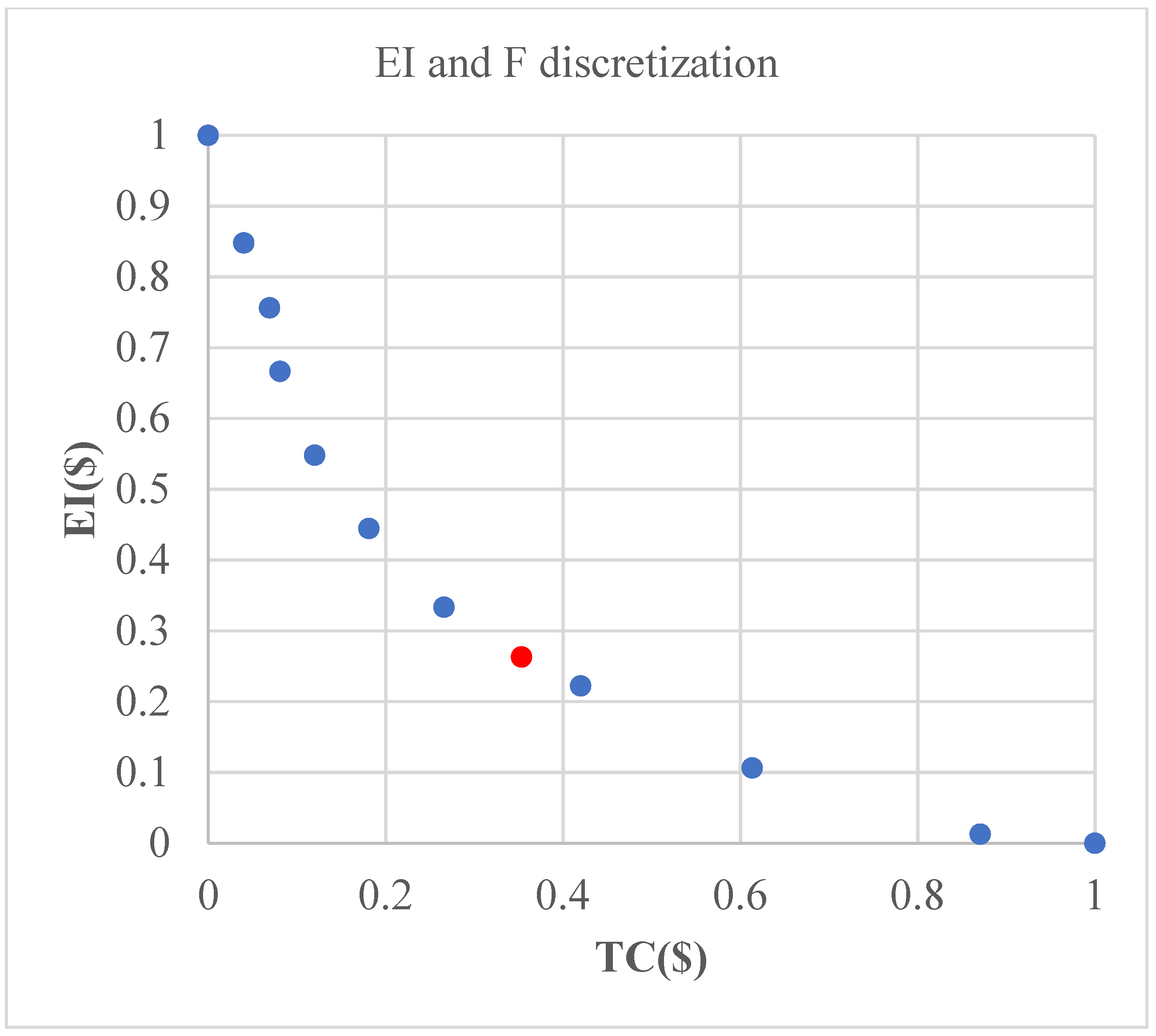
EI and TC Discretization

In multi-objective optimization, especially when minimizing both environmental impact (EI) and total cost (TC), achieving a well-distributed Pareto front is essential for understanding the trade-offs between conflicting objectives. In the initial approach, the goal programming model results failed to produce a comprehensive Pareto front curve. This indicates that the solutions were clustered or limited in variety, failing to capture the full range of trade-offs that exist between cost and environmental performance.

Discretizing only one objective, such as environmental impact, essentially anchors the optimization process around fixed intervals or target values for that single objective, while allowing the other (in this case, total cost) to adjust freely. However, this often results in a biased or incomplete representation of the solution space, particularly when the free objective has a dominant influence over the optimization process. This can lead to solutions that are technically feasible but suboptimal in terms of the balance between objectives or that fail to adequately explore areas of the trade-off curve where decision makers might find more favorable compromises.

To address this limitation, it becomes necessary to also discretize the total cost by systematically varying target values for total cost and incorporating them as constraints in the goal programming model like case I. This dual discretization ensures that both objectives are equally emphasized in the optimization process, allowing the algorithm to generate a more complete and well-distributed set of Pareto-optimal solutions. According to this approach, in Figure 6, point J (red point) is obtained, which is the optimal point for both total cost and environmental impact.

The network configuration of point J represented in Figure 7 and the shows a more strategically balanced resource allocation achieved through the application of a quantity discount schedule. This new configuration signifies a shift toward an optimized solution that addresses both cost and environmental impact in a more integrated manner.

At point J, manufacturing center, Dire Dawa sources vegetables from Jimma, while the Bahir Dar center procures its supply from West Shewa using quantity discount (see Figure 7). Sidama and Bulbula purchased the vegetable from multiple supplies without quantity discount. This configuration contrasts sharply with the earlier scenario, In Case I, manufacturing centers such as Sidama, located in proximity to major suppliers, benefited from quantity discounts by sourcing from adjacent supply nodes. This configuration, represented by scenario K, (see Figure 4) corresponds to the ideal (utopia) point in the multi-objective solution space, where both total cost and environmental impact are minimized.

In Case II, the decision to source vegetables from more distant suppliers, such as Dire Dawa sourcing from Jimma and Bahir Dar sourcing from West Shewa, introduces a more deliberate and strategic approach to resource allocation. By utilizing the quantity discount mechanism, this approach aims not only to reduce the total cost but also to mitigate the environmental impact more effectively. The decision to select suppliers that are farther away increases transportation distances and costs but is balanced by the savings achieved through bulk purchasing under the quantity discount strategy. The optimization process successfully incorporates both economic and environmental factors, ensuring that the supply chain is both cost-efficient and environmentally responsible. By considering both dimensions of performance, this allocation corrects the earlier oversights and leads to a more sustainable solution.

This improved sourcing strategy contributes to a more equitable trade-off between TC and EI, effectively offsetting the limitations of Case I. It demonstrates the importance of spatial and economic considerations in supply chain design and highlights how carefully structured procurement strategies, especially when incorporating quantity discount policies, can serve as powerful levers in multi-objective decision making, enhancing the overall sustainability and resilience of the supply chain network.

In

Table 4. EI and TC discretization.

	Pareto Front Absolute		Pareto Front Relative		CPU Time (min), Intel 2.80-GHz
Scenario	TC ($)	EI ($)	TC	EI
	52.634	112.25	0	1
A	52.634	112.25	0	1	0.68
B	52.789	105.69	0.04009312	0.84807781	46
C	52.901	101.72	0.06906363	0.7561371	75
D	52.947	97.85	0.08096223	0.66651227	27
E	53.098	92.737	0.12002069	0.54810097	244
F	53.334	88.26	0.1810657	0.44441871	155
G	53.662	83.466	0.26590792	0.33339509	17
H	54.258	78.666	0.42007243	0.22223252	148
I	55.006	73.666	0.61355406	0.10643817	1579
J	54	80.43	0.35333678	0.26308476	1836
K	56	69.625	0.87066736	0.01285317	1139
	56.5	69.07	1	0

The value highlighted in yellow at the top represents the minimum total cost (TC) and the maximum environmental impact (EI) while executing the multi-objective function without considering any constraints. In contrast, the value at the bottom of the table represents the maximum total cost (56.5) and the minimum environmental impact (EI) subject to constraints. Furthermore, the value in row J indicates the optimal values of both functions determined using goal programming.

, a revision was made to the maximum total cost (TC) value employed in the analysis. Initially, the payoff table (Table 2) reported a maximum TC of 83.684. However, through the discretization of the total cost values, an alternative TC value ranging between 52.634 and 83.628 was identified, corresponding to a minimum environmental impact (EI) value of 69.07. By establishing a threshold whereby TC is greater than or equal to 56.5, this new maximum value of 56.5 was adopted. This adjustment was intended to eliminate excessively high-cost scenarios and to concentrate the analysis on more practical and feasible solutions. Under this revised threshold, the corresponding EI was observed to attain its minimum value of 69.07. To enhance the robustness of the analysis, the simulation results were subsequently normalized, thereby enabling clearer and more meaningful patterns to emerge across the different scenarios, as presented in the relative Pareto front in Table 4.

Building on these updated conditions, an additional solution, referred to as point J, was identified using goal programming, as depicted in Figure 6. This point is chosen as the optimal solution. Goal programming helped to balance the dual objectives of minimizing both TC and EI under the revised, more realistic constraints. Point J represents a compromise solution that was not apparent in the original payoff table but became visible after discretization of TC. This process ultimately improved the interpretability of the simulation outcomes and highlighted more feasible trade-offs between cost and environmental impact.

Compared to scenario A, scenario J achieves a 28% reduction in EI due to optimized sourcing and transportation efficiency, though this comes at a 2% increase in total cost. As a non-dominated solution on the Pareto front, scenario J represents a trade-off where a significant environmental improvement is attained with only a marginal rise in cost. This positioning suggests that scenario J is closer to an optimal point, where further reductions in EI may lead to disproportionately higher costs. Scenario j optimizes the network configuration to maximize quantity discounts, outperforming all other scenarios.

This resolution strategy not only reduces computational effort but also offers decision makers a clear view of the trade-offs between economic and environmental objectives. By structuring the optimization process in this way, it becomes easier to assess the impact of prioritizing one criterion over the other, thereby facilitating more informed decision making. Consequently, scenario j addresses this challenge by strategically selecting distant locations, such as Dire Dawa and Bahir Dar, and leveraging a quantity discount strategy to balance the additional costs associated with these locations (Figure 7).

Extrapolating the perishable food supply chain model developed for Ethiopia to other countries is essential for addressing global food security challenges. This process involves understanding local contexts, including market dynamics and cultural factors, while also analyzing agri-food structures such as infrastructure and regulatory environments. Gathering relevant local data is crucial for adapting the model effectively, and collaboration with local experts ensures its accuracy and relevance. A modular design allows for flexibility, enabling adjustments to meet specific needs, and pilot testing helps refine the model’s effectiveness in real-world situations. By documenting best practices from the Ethiopian case, we can guide its application in diverse contexts.

6. Conclusions

This study presents a multi-objective optimization approach for the perishable food supply chain network by integrating both economic and environmental considerations. The proposed model addresses the complexities of a multi-period, multi-sourcing, and multi-product supply chain, ensuring that decision making reflects real-world challenges in food supply chain design. By optimizing total cost and environmental impact, the model provides valuable insights into perishable food supply chain management.

The findings of this multi-objective optimization study were analyzed through two distinct scenarios (Case I and Case II) to examine the effectiveness of combining the epsilon constraint method with goal programming in capturing the trade-offs between cost minimization and environmental impact reduction within a perishable food supply chain. In Case I, the environmental impact objective was discretized into multiple intervals, and the epsilon constraint method was applied. However, this approach resulted in a limited number of points along the Pareto front and required an extensive computation time of approximately 24 h. To address these limitations, the methodology was extended by integrating goal programming, which produced an additional solution point (Point K). Despite this improvement, the results indicate that the antagonistic relationship between cost and environmental objectives was still not fully captured, underscoring the need for more balanced discretization and advanced optimization strategies to better represent the trade-offs in complex supply chain networks.

In Case II, the optimization process was extended by incorporating the discretization of total cost (TC), which allowed for a more nuanced exploration of the trade-offs between cost and environmental impact (EI). By discretizing TC, the model was able to strategically select distant locations for sourcing, such as Dire Dawa and Bahir Dar, rather than relying on nearby suppliers. This geographic diversification facilitated the leveraging of quantity discounts, which provided cost savings while simultaneously spreading out the environmental impact across a broader area. This approach not only refined the optimization process but also ensured a more balanced allocation of resources between the two conflicting objectives of minimizing cost and reducing environmental impact. The solution obtained in Case II, represented by Point J, demonstrates the practical benefits of this strategy. Notably, as shown in Figure 5, the red point indicates a solution that successfully reduces environmental impact (EI) by 28% while only increasing total cost (TC) by 2%. This result highlights the effectiveness of the discretization of TC and the strategic selection of supplier locations, showcasing a significant improvement over the previous solution (case I). The slight increase in TC is a small trade-off when compared to the substantial reduction in EI, reflecting a more sustainable and cost-effective configuration for the supply chain.

This research examined the impact of using integrated solution methods for operational research applied to the perishable food supply chain network design model, with a focus on long-term sustainability from both economic and environmental perspectives. By employing an integrated epsilon constraint model in conjunction with goal programming, we achieved Pareto-efficient solutions while significantly reducing resolution time. In contrast, using the epsilon constraint method alone resulted in lengthy computation times exceeding 24 h and did not produce Pareto-efficient outcomes.

Future research should expand the scope of multi-objective optimization by incorporating operational decision making, particularly the vehicle routing problem (VRP), to further enhance supply chain efficiency. Integrating the VRP would allow for a more detailed and realistic representation of logistics, considering factors such as transportation costs, delivery times, and environmental impact in the routing process.

References

1. Reavis, M.; Ahlen, J.; Rudek, J.; Naithani, K. Evaluating Greenhouse Gas Emissions and Climate Mitigation Goals of the Global Food and Beverage Sector. Front. Sustain. Food Syst. 2022, 5, 789499. [Google Scholar] [CrossRef]
2. Castillo-Díaz, F.J.; Belmonte-Ureña, L.J.; López-Serrano, M.J.; Camacho-Ferre, F. Assessment of the sustainability of the European agri-food sector in the context of the circular economy. Sustain. Prod. Consum. 2023, 40, 398–411. [Google Scholar] [CrossRef]
3. MoA, Ministry of Agriculture. Transforming Ethiopian Agriculture, Briefing for Agricultural Scholars Consultative Forum. United Nations Conference Center. Addis Ababa (UNCC), April 2019. Available online: https://citizenengagement.nepad.org/pdf/20231005145754.pdf (accessed on 19 November 2022).
4. Esteso, A. Conceptual framework for designing agri-food supply chains under uncertainty by mathematical program. Int. J. Prod. Res. 2018, 56, 4418–4446. [Google Scholar] [CrossRef]
5. Soto-Silva, W.E.; Nadal-Roig, E.; Gonz´alez-Araya, M.C.; Pla-Aragones, L.M. Operational research models applied to the fresh fruit supply chain. Eur. J. Oper. Res. 2016, 251, 345–355. [Google Scholar] [CrossRef]
6. Gustavsson, J.; Cederberg, C.; Sonesson, U. Global Food Losses and Food Waste: Extent, Causes, and Prevention; Food and Agriculture Organization of the United Nations (FAO): Rome, Italy, 2022. [Google Scholar]
7. Osman, S.A.; Xu, C.; Akuful, M.; Paul, E.R. Perishable Food Supply Chain Management: Challenges and the Way Forward. Open J. Soc. Sci. 2023, 11, 349–364. [Google Scholar] [CrossRef]
8. Hidayati, D.R. Enabling sustainable agrifood value chain transformation in developing countries. J. Clean. Prod. 2023, 395, 136300. [Google Scholar] [CrossRef]
9. Rahbari, M.; Khamseh, A.A.; Mohammadi, M. Robust optimization and strategic analysis for agri-food supply chain under pandemic crisis: Case study from an emerging economy. Expert Syst. Appl. 2023, 225, 120081. [Google Scholar] [CrossRef]
10. Yaghoubi, A.; Akrami, F. Proposing a new model for location—Routing problem of perishable raw material suppliers with using meta-heuristic algorithms. Heliyon 2019, 5, e03020. [Google Scholar] [CrossRef]
11. Paredes-Rodríguez, A.M.; Osorio-Gómez, J.C.; Orejuela-Cabrera, J.P. Dynamic evaluation of distribution channels in a fresh food supply chain from a sustainability and resilience approach. Alex. Eng. J. 2024, 106, 42–51. [Google Scholar] [CrossRef]
12. Pan, L.; Shan, M. Optimization of Sustainable Supply Chain Network for Perishable Products. Sustainability 2024, 16, 5003. [Google Scholar] [CrossRef]
13. Nasiri, M.M.; Mousavi, H.; Nosrati-Abarghooee, S. A green location-inventory-routing optimization model with simultaneous pickup and delivery under disruption risks. Decis. Anal. J. 2023, 6, 100161. [Google Scholar] [CrossRef]
14. Mousavi, R.; Bashiri, M.; Nikzad, E. Stochastic production routing problem for perishable products: Modeling and a solution algorithm. Comput. Oper. Res. 2022, 142, 105725. [Google Scholar] [CrossRef]
15. Manouchehri, F.; Nookabadi, A.S.; Kadivar, M. Production routing in perishable and quality degradable supply chains. Heliyon 2020, 6, e03376. [Google Scholar] [CrossRef] [PubMed]
16. Liu, L.; Zhao, Q.; Santibanez Gonzalez, E.D.R.; Xi, X. Sourcing and production decisions for perishable items under quantity discounts and its impacts on environment. J. Clean. Prod. 2021, 317, 128455. [Google Scholar] [CrossRef]
17. Komijani, M.; Sajadieh, M.S. An integrated planning approach for perishable goods with stochastic lifespan: Production, inventory, and routing. Clean. Logist. Supply Chain 2024, 12, 100163. [Google Scholar] [CrossRef]
18. Huang, X.; Yang, S.; Wang, Z. Optimal pricing and replenishment policy for perishable food supply chain under inflation. Comput. Ind. Eng. 2021, 158, 107433. [Google Scholar] [CrossRef] [PubMed]
19. Grillo, H.; Alemany, M.M.E.; Ortiz, A.; Fuertes-Miquel, V.S. Mathematical modelling of the order-promising process for fruit supply chains considering the perishability and subtypes of products. Appl. Math. Model. 2017, 49, 255–278. [Google Scholar] [CrossRef]
20. Gioia, D.G.; Felizardo, L.K.; Brandimarte, P. Simulation-based inventory management of perishable products via linear discrete choice models. Comput. Oper. Res. 2023, 157, 106270. [Google Scholar] [CrossRef]
21. Esteso, A.; Alemany, M.M.E.; Ortiz, Á. Impact of product perishability on agri-food supply chains design. Appl. Math. Model. 2021, 96, 20–38. [Google Scholar] [CrossRef]
22. Ekanayake, C.; Bandara, Y.M.; Chipulu, M.; Chhetri, P. An order fulfilment location planning model for perishable goods supply chains using population density. Supply Chain Anal. 2023, 4, 100045. [Google Scholar] [CrossRef]
23. Ge, H.; Goetz, S.J.; Cleary, R.; Yi, J.; Gómez, M.I. Facility locations in the fresh produce supply chain: An integration of optimization and empirical methods. Int. J. Prod. Econ. 2022, 249, 108534. [Google Scholar] [CrossRef]
24. de Keizer, M.; Haijema, R.; Bloemhof, J.M.; van der Vorst, J.G.A.J. Hybrid optimization and simulation to design a logistics network for distributing perishable products. Comput. Ind. Eng. 2015, 88, 26–38. [Google Scholar] [CrossRef]
25. Hiassat, A.; Diabat, A.; Rahwan, I. A genetic algorithm approach for location-inventory-routing problem with perishable products. J. Manuf. Syst. 2017, 42, 93–103. [Google Scholar] [CrossRef]
26. Abbasian, M.; Sazvar, Z.; Mohammadisiahroudi, M. A hybrid optimization method to design a sustainable resilient supply chain in a perishable food industry. Environ. Sci. Pollut. Res. 2023, 30, 6080–6103. [Google Scholar] [CrossRef]
27. Miao, X.; Pan, S.; Chen, L. Optimization of perishable agricultural products logistics distribution path based on IACO-time window constraint. Intell. Syst. Appl. 2023, 20, 200282. [Google Scholar] [CrossRef]
28. Govindan, K.; Jafarian, A.; Khodaverdi, R.; Devika, K. Two-echelon multiple-vehicle location–routing problem with time windows for optimization of sustainable supply chain network of perishable food. Int. J. Prod. Econ. 2014, 152, 9–28. [Google Scholar] [CrossRef]
29. Soto-Silva, W.E.; González-Araya, M.C.; Oliva-Fernández, M.A.; Plà-Aragonés, L.M. Optimizing fresh food logistics for processing: Application for a large Chilean apple supply chain. Comput. Electron. Agric. 2017, 136, 42–57. [Google Scholar] [CrossRef]
30. Jonkman, J.; Barbosa-Póvoa, A.P.; Bloemhof, J.M. Integrating harvesting decisions in the design of agro-food supply chains. Eur. J. Oper. Res. 2019, 276, 247–258. [Google Scholar] [CrossRef]
31. Biza, A.; Montastruc, L.; Negny, S.; Admassu, S. Strategic and tactical planning model for the design of perishable product supply chain network in Ethiopia. Comput. Chem. Eng. 2024, 190, 108814. [Google Scholar] [CrossRef]
32. Biuki, M.; Kazemi, A.; Alinezhad, A. An integrated location-routing-inventory model for sustainable design of a perishable products supply chain network. J. Clean. Prod. 2020, 260, 120842. [Google Scholar] [CrossRef]
33. Rajabi, R.; Shadkam, E.; Khalili, S.M. Design and optimization of a pharmaceutical supply chain network under COVID-19 pandemic disruption. Sustain. Oper. Comput. 2024, 5, 102–111. [Google Scholar] [CrossRef]
34. Klöpffer, W. (Ed.) Background and Future Prospects in Life Cycle Assessment; Springer: Dordrecht, The Netherlands, 2014. [Google Scholar]
35. Reyes, T.; Gouvinhas, R.P.; Laratte, B.; Chevalier, B. A method for choosing adapted life cycle assessment indicators as a driver of environmental learning: A French textile case study. Anal. Manuf. 2020, 34, 68–79. [Google Scholar] [CrossRef]
36. Üçtuğ, F.G.; Tekin, Z.; Dayıoğlugil, Z.; Ulusoy, E.; Oktaylar Keyik, Ş. Life cycle assessment of tomato paste production: A case study. J. Eng. Sci. 2024, 30, 119–127. [Google Scholar] [CrossRef]
37. Vogtländer, J.G.; Bijma, A. The ‘virtual pollution costs ‘99’, a single LCA-based indicator for emissions. Int. J. Life Cycl. Assess. 2000, 5, 13–124. [Google Scholar]
38. Eslami, E.; Abdurrahman, E.; Pataro, G.; Ferrari, G. Increasing sustainability in the tomato processing industry: Environmental impact analysis and future development scenarios. Front. Sustain. Food Syst. 2024, 8, 1400274. [Google Scholar] [CrossRef]
39. Teferra, T.F. The cost of postharvest losses in Ethiopia: Economic and food security implications. Heliyon 2022, 8, e09077. [Google Scholar] [CrossRef] [PubMed]
40. Maroulis, Z.B.; Saravacos, G.D. Food Processing Design. Available online: https://books.tarbaweya.org/static/documents/uploads/pdf/Food%20Process%20Design%20by%20Zacharias%20B.%20Maroulis%2C%20George%20D.%20Saravacos%20(z-lib.org).pdf (accessed on 3 March 2021).
41. Miret, C.; Chazara, P.; Montastruc, L.; Negny, S.; Domenech, S. Design of bioethanol green supply chain: Comparison between first and second-generation biomass concerning economic, environmental and social criteria. Comput. Chem. Eng. 2016, 85, 16–35. [Google Scholar] [CrossRef]
42. Parin, M.A.; Zugarramurdi, A. Investment and production costs analysis in food processing plants. Int. J. Prod. Econ. 1994, 34, 83–89. [Google Scholar] [CrossRef]
43. Abiso, E.; Satheesh, N.; Hailu, A. Effect of storage methods and ripening stages on postharvest quality of tomato (Lycopersicom esculentum Mill) CV. Chali. Ann. Food Sci. Technol. 2015, 16, 127–137. [Google Scholar]
44. Kitinoja, L. Exploring the Potential for Cold Chain Development in Emerging and Rapidly Industrializing Countries. 2014. Available online: https://www.researchgate.net/publication/294259640_Exploring_the_potential_for_cold_chain_development_in_emerging_and_rapidly_industrializing_countries (accessed on 19 November 2022).
45. Ramos, M.A.; Boix, M.; Montastruc, L.; Domenech, S. Multi objective Optimization Using Goal Programming for Industrial Water Network Design. Ind. Eng. Chem. Res. 2014, 53, 17722–17735. [Google Scholar] [CrossRef]
Figure 1. Model superstructure.
Logistics 09 00080 g001
Figure 2. Schematics of the multi-objective optimization.
Logistics 09 00080 g002
Figure 3. Map of point K for Case I.
Logistics 09 00080 g003
Figure 4. Pareto front curve for EI discretization.
Logistics 09 00080 g004
Figure 5. Strategic network configuration of PFSC.
Logistics 09 00080 g005
Figure 6. Pareto front curve for EI and TC discretization.
Logistics 09 00080 g006
Figure 7. Map of point J for Case II.
Logistics 09 00080 g007