Abstract
Background: We consider a variant of the traveling salesperson problem motivated by the case of a company delivering furniture. The problem is both dynamic, due to random arrivals of delivery requests, and multiperiod, due to flexibility in delivering items within a time window of a few days. A sequence of daily routes must be selected over time, and both volume and route duration constraints are relevant. Moreover, customers are irregularly distributed in clusters with high or low density. When receiving a request from a low-density cluster, we may consider the possibility of waiting for further requests from the same cluster, which involves a tradeoff between total traveled distance and service quality. Methods: We designed alternative decision policies based on approximate dynamic programming principles. We compared policy and cost function approximations, tuning their parameters by simulation-based optimization. Results: We compared the decision policies by realistic out-of-sample simulations. A simple trigger-based decision policy was able to achieve a good compromise among possibly conflicting objectives, without resorting to full-fledged multiobjective models. Conclusions: The insights into the relative strengths and weaknesses of the tested policies pave the way to practical extensions. Due to its computational efficiency, the trigger policy may be improved by base-policy rollout and integrated within a multi-vehicle routing architecture.
1. Problem Description and Motivation
We consider a dynamic, stochastic, and capacitated version of the traveling salesperson problem (TSP), whose main features are as follows:
- There is a stochastic stream of customer requests over time. On each day, new customers join the waiting queue for delivery.
- Each request is associated with a volume, a service time, and a due date (in days).
- The traveling salesperson, which is actually a vehicle, is subject to a volume capacity constraint. However, there is also a constraint on the tour duration within a day, as there is not only a delivery but also a service component. The sum of service times (on nodes) and traveling times (on arcs) must be smaller than the maximum allowed tour duration within each day.
- Since there are capacity constraints, it may not be possible to serve all of the requests waiting in the queue in a single day. Moreover, it may not be advisable, as customers are not uniformly distributed in space. On the contrary, customers are clustered. Besides a high-density cluster close to the deposit, there are low-density clusters, which are much less convenient to serve in terms of traveled distance.
- The presence of such low-density clusters suggests the potential opportunity of delaying service to inconvenient customers, within the allowed time window for delivery, waiting for more requests from the same cluster.
- Given the stochastic stream of arrivals, we face a difficult decision problem that, in principle, might be decomposed into two components: the dispatching decision, i.e., the selection of a subset of waiting requests to satisfy during the current day, and the routing decision, i.e., the choice of a route for the current day, to minimize the traveled distance.
- Unfortunately, the presence of a constraint on tour duration does not allow for a pure cluster-first/route-second strategy. We have to devise a policy to tackle this sequential decision problem under uncertainty in order to minimize the long-run average of the traveled distance per day.
- Even though the main objective is minimizing traveled distance, we should also keep customer service under control. This means avoiding late deliveries and possibly reducing waiting times. Hence, the overall problem is multiobjective, but it is difficult to define weights measuring the relative importance of conflicting objectives.
The TSP version that we consider may be labeled as Multiperiod Dynamic Capacitated TSP (MDCTSP for short). We will clarify why it is important to emphasize both multiperiod and dynamic features later, when we compare our problem with the literature on dynamic vehicle routing problems (VRPs).
1.1. Practical Motivation
The practical motivation, justifying the problem features that we have just described, arises from the actual case of a firm selling pieces of furniture that are loaded at a central warehouse and delivered to customers by trucks. The kinds of items, unlike in the case of small parcels, imply that the volume constraint may be relevant and that delivery routes are planned a day ahead and then executed without online adjustment (unlike parcel pickup and delivery). Moreover, the vehicle crew is also in charge of assembling the delivered items on site, if needed. Hence, there is a significant service component, and the maximum allowed total route duration is a relevant constraint. Each route starts in the morning at the warehouse and is completed within the day by returning to it. In practice, a vehicle does not execute multiple routes within the day. The problem is multiperiod, since a sequence of daily routes is produced based on the current queue of waiting customers and their delivery due dates. When a delivery becomes eligible, i.e., when the request joins the waiting queue, it is associated with a time window of a few days (the length of the time window may be different for more or less urgent deliveries). Hence, the route planners have to decide on which day it is best to serve a request, without violating its due date. Last but not least, the warehouse is located close to a large town, which provides a high-density cluster of customers, but there are smaller towns nearby, which are low-density clusters. A difficult task for route planners it to decide whether to serve an inconvenient request from a low-density cluster immediately, or to wait for additional requests from the same zone. This also depends on the load associated with a request, since there may be little point in waiting, when a single request saturates the truck capacity.
In this dynamic and uncertain context, route planners have to make two interrelated decisions:
- 1.
- The dispatching decision, i.e., the selection of the subset of waiting customers to serve during the next day;
- 2.
- The routing decision, i.e., the selection of a feasible route for each available vehicle (the number of available trucks is fixed).
The task is complicated by the need to strike a balance between the objective of minimizing traveled distance and customer waiting times without missing due dates.
1.2. Scientific Motivation
The practical problem that we have just described is one of many possible variants of the classical capacitated vehicle routing problem (CVRP). See, e.g., [1] for a comprehensive survey of VRPs. Even in its basic form, the CVRP is a hard combinatorial optimization problem, and heuristic approaches must be used to find high-quality solutions [2]. The classical CVRP is a deterministic and static problem, since all the data are known and the whole set of customers must be served immediately. In a multiperiod problem, there is a time horizon, consisting of a few time periods, and we may choose on which day each delivery may be executed, possibly under a due date constraint [3]. It is important to note that, per se, the multiperiod VRP is a static problem under the assumption that the whole set of customers is known at the current time. In practice, the problem is solved according to a rolling horizon strategy, whereby additional customers are added to the pool of delivery requests, and the problem is solved repeatedly. However, unlike multistage decision problems, in a static multiperiod setting the possibility of revising decisions is not explicitly accounted for within the model. A large body of research, on the contrary, deals with dynamic VRPs [4]. A dynamic and online variant of VRP occurs when service requests (e.g., parcel pickups and deliveries) are observed in real time, and we must decide whether to accept or reject each new request. If accepted, the request must be inserted into a current vehicle route, taking current vehicle locations into account. Usually, when dealing with small items, the volume capacity is not binding, but the total route time is subject to a duration constraint. This problem is dynamic, and it needs to account for the system state, which consists of the current set of routes, the current vehicle positions, and the list of accepted, while still waiting for requests. The objective may be the maximization of profit derived from accepted requests, subject to total traveled time constraints (there is a possible penalization for total traveled distance). This kind of problem is dynamic but not multiperiod, since deliveries are planned within a single day and the decisions are relatively simple, as they involve the possible insertion of a single request. In the literature, there is a rich variety of dynamic routing problems under uncertainty. See, e.g., [5] for an inventory routing problem involving perishable items.
On the one hand, the practical problem that we have described is stochastic and dynamic, as there is a clear state component (the pool of waiting customers) and each decision has an uncertain impact on future decisions. On the other hand, it is also multiperiod, as it involves planning over multiple days. Complicating features include twofold capacity constraints, multiple objectives, and clustered customers. To the best of our knowledge, this precise combination of features has not been investigated in the literature on VRPs, even though each individual feature has been dealt with. Hence, there is a strong motivation to consider this variant.
1.3. Our Contributions
We should note that, after making the dispatching decision, the routes may be post-optimized by solving a fairly standard CVRP subproblem. The clearly challenging part is selecting the subset of customers to be served the next day from the waiting pool. In order to better focus on this side of the coin, in this paper, we address a simplified version of the practical problem, i.e., the single-vehicle case, which boils down to a capacitated TSP problem. As we will argue later, this is a necessary and essential methodological step in order to get a clearer picture by comparing different principles of approximate dynamic programming to the dispatching decision. We will also propose a natural way to extend the proposed approach to the more realistic case of multiple vehicle.
Notwithstanding this limitation, our contributions can be summarized as follows:
- We consider a practically relevant version of a multiperiod, stochastic, and dynamic routing problem, which differs from other variants discussed in the literature.
- We show that, by using simulation-based optimization to fine-tune the parameters of a simple decision policy, we can devise a strategy that outperforms naive heuristics and another, seemingly more sophisticated strategy.
- We take a pragmatic approach, showing that we can find a good compromise among conflicting objectives (meeting delivery deadlines, limiting customer waiting times, and finding efficient routes), without resorting to the problematic machinery of multiobjective optimization.
- Even though we consider a simple illustrative case in our experiments, the results are practically relevant. The proposed solution strategy, after tuning its parameters, is quite fast, which implies that:
- 1.
- it can easily scaled and adapted to the more realistic case of multiple vehicles;
- 2.
- it provides us with a base heuristic that may be embedded within lookahead-based strategies, where policy rollout may further improve its performance.
1.4. Structure of the Paper
The paper is structured as follows. We provide a brief review of the relevant literature in Section 2 in order to provide the necessary background and to further position our paper. The overall problem is formalized within the framework of stochastic dynamic programming in Section 3, where we also describe the essential building blocks of approximate solution strategies, most notably policy function and cost function approximations. We apply such strategies to a pilot case study that is described in Section 4. A possible implementation of a policy function approximation strategy is described in Section 5, whereas a cost function approximation approach is the subject of Section 6. The computational results are discussed in Section 7. Section 8 outlines possible strategies to expand the method from the TSP to the VRP setting, followed by conclusions in Section 9.
2. Background and Paper Positioning
In this section, we first summarize the relevant concepts concerning approximate dynamic programming, like value function, cost function, and policy function approximations, as well as lookahead strategies. Then, based on this background, we frame some approaches to dynamic VRPs that have been proposed in the literature, limiting the discussion to the references that are more related to our case study. In this paper, we tackle the single vehicle case (capacitated TSP), but it is important to consider the literature on the more general case of multiple vehicles (VRP). Finally, we position our paper in terms of problem setting and solution approach, pointing out similarities and differences with respect to the literature.
2.1. Approximate Dynamic Programming Strategies
Stochastic dynamic programming (SDP) is a general framework for casting a wide variety of sequential decision problems under uncertainty [6,7]. Formally, we consider a discrete time index t and define the following:
- A state variable , possibly a high-dimensional vector, collecting all of the necessary information to make a decision at time t, while accounting for its consequences;
- A decision variable , representing the decision made at time t, after observing the current state ;
- An exogenous piece of information , which is a random variable representing the realization of uncertain factors during the time interval from time instant t to time instant .
The system dynamics are characterized by a state transition function giving the next state as
Typically, constraints are enforced on decisions, so that we must consider . The set , in general, may depend on the state, and constraints on states may also be necessary, but this will not be the case in our paper. The time subscript in emphasizes that the new information is not known when we make decision . This is the most common assumption, but it is not necessarily true when some lookahead is available; indeed, as we shall discuss in Section 3, we may observe the newly arrived delivery requests before making the routing decision for the current day, but we do not know which further delivery requests are going to arrive during the day, to be served on future days (see, e.g., [6] for a discussion of this point and other practical examples). Here, we assume that the form of the transition equation does not change with time. We will be more specific about the definition of states and decisions, as well as the timing of exogenous uncertainty, in Section 3, where we specialize the framework to our problem.
The decision has an impact on the next state and on the immediate reward (or cost) collected at time t, which may be represented as or , depending on whether the immediate reward is deterministic or not. In the problem we deal with, the first case applies. Since the sequence of decisions adapts to a random state evolution, each is a random variable as well. We look for a decision policy , i.e., a mapping prescribing a feasible decision for each state: . Let denote the set of feasible policies.
In order to find an optimal policy (which may not be unique), we should solve a problem like
i.e., an infinite-time discounted problem, where is a discount factor needed to ensure convergence of the series. Since in our problem there is no definite time horizon, we look for a stationary policy over an infinite time horizon. Note that when learning a policy based on the simulation of a suitably long but finite-horizon sample path, the discount factor may be disregarded and set to 1.
The standard dynamic programming approach relies on a value function , which is the expected total discounted reward if we start from state and apply an optimal policy. It can be shown that, under reasonable assumptions, the value function satisfies the recursive Bellman equation,
for every state . In practice, a direct approach for solving a dynamic stochastic problem based on the Bellman equation is not feasible, since the state is high-dimensional (and it is certainly so in a VRP).
Hence, we have to resort to approximate dynamic programming (ADP) strategies. There is a huge variety of such strategies, but they can be interpreted in terms of four basic approaches [8].
- 1.
- Value function approximation (VFA). The trouble with Equation (2) is that it relies on a value function that must be defined for every possible state. When the state space is continuous, the value function lives in an infinite-dimensional space, but even if the state space is discrete, its sheer size and the resulting curse of state dimensionality require some form of approximation. A typical way to discretize the problem, or to limit its dimensionality, is to project the value function onto a smaller function space, which may be accomplished by considering linear combinations of a set of given basis functions. The coefficients of the linear combination may be learned, e.g., by simulation and linear regression. More generally, we may consider parametric value function approximations that need not be linear combinations; see, e.g., [9] for a survey. Alternative non-parametric approaches rely, e.g., on state aggregation. The use of neural networks is also common, in which case the number of parameters is so large that the approach can be considered, in a sense, non-parametric. There are numerous computational approaches for learning a suitable approximation of the value function. Still, they require a significant computational effort, as well as ingenious customization to the problem at hand.
- 2.
- Cost function approximation (CFA). Dynamic programming is a strategy for avoiding myopic decisions resulting from a greedy approach, whereby we only care about immediate reward. We can do so by introducing a value function and solving a single-stage problem, but a computationally cheaper alternative is to modify the immediate reward (or cost) to account for the later impact of current choices. This idea leads to the cost function approximation approach. Again, parameters may be introduced into the approximation, and their value can be learned by simulation-based optimization.
- 3.
- Policy function approximation (PFA). The value function in itself may provide useful information, but it is usually instrumental in determining a policy. Indeed, a good approximation of the value function is often sufficient to derive a satisfactory policy. An alternative approach aims at directly finding an approximated policy function , mapping each state to a decision . Such policies may be simple rules of thumb, parameterized decision rules, or even actor neural networks. Simulation-based optimization may be used to fine-tune the parameters of simple decision rules, as we shall see in the following.
- 4.
- Limited lookahead. Several classical SDP algorithms, like policy iteration, require assessing the value function associated with a policy, not necessarily the optimal one. This may be a computationally intensive task, but we may obtain a suitable approximation by direct lookahead, i.e., by simulating the application of this approximate (base) policy over a limited number of steps. One way to leverage the idea and to improve the base policy is to compare different decisions by summing the immediate rewards collected over such a limited horizon and an estimate of the value function in the last state, provided by a limited lookahead relying on the application of the base policy. We may do so using Monte Carlo tree search strategies [10] or rollout methods, which may be integrated with PFA [11].
We should highlight that these four principles may be combined in a wide array of hybrid strategies, as documented by a huge amount of literature, also comprising reinforcement learning approaches [12]. In the next section, we outline how such ideas have been adapted to different versions of the dynamic VRP.
2.2. A Miscellanea of Dynamic VRPs
Recently, there has been a surge of papers applying machine learning to VRPs [13], as well as approximate dynamic programming to dynamic VRPs [14] specifically, and to transportation and logistics in general [15]. It is useful to pinpoint the basic features that may be used to classify the problems addressed by such literature. A VRP may be
- stochastic or deterministic;
- static or dynamic;
- online or offline;
- multiperiod or single-period;
- characterized or not by spatial and/or temporal heterogeneity.
To appreciate the relevance of these features, it is useful to consider the problem addressed by [3], which is a multiperiod VRP with due dates. A set of routes must be developed for each day within a given time horizon, accounting for customer due dates constraining the days on which delivery can be executed without incurring any penalty. The problem is multiperiod but static, as the set of orders does not change over time, and there is no uncertainty involved. This allows the application of very sophisticated mixed-integer linear programming strategies to find the optimal solution, at least in limited size problems. In contrast, a radically different problem is considered, e.g., in [16], where a dynamic, online, same-day service/delivery problem is addressed. The problem is stochastic, since requests arrive according to a Poisson process and can be accepted or postponed to a later period, which makes the problem multiperiod in a limited sense. In other papers, requests may just be accepted or rejected, and the problem does not span multiple periods. In papers like [16], the route is developed and adjusted online, which makes sense for pickup/delivery or service problems but is not applicable if bulky items must be collected from a deposit. Moreover, spatial heterogeneity is considered in [16], since customers issuing requests are clustered in two or three clusters and distributed according to a normal or uniform distribution within each cluster. Since clusters may be more or less convenient to visit, the issue of equitable service levels is also discussed. A problem that is both dynamic and multiperiod is considered in [17], where full routes must be developed for a sequence of days, but there is a random stream of requests, which requires careful decisions about the set of customers that are selected for immediate service. The problem considered by [17] is quite similar to what we consider here. The main difference is that we do not consider a fixed set of customers. If requests are randomly issued by a fixed set of customers, reliable probabilistic information may be obtained about their timing, which may be used to quantify the suitability of each customer for immediate service. We do not assume the availability of such reliable information. Moreover, we compare alternative solution strategies based on dynamic programming.
2.3. ADP for Dynamic VRPs
Even the tiny set of examples in the previous section is enough to appreciate how dynamic and/or multiperiod VRPs span a wide variety of problems, with a clear impact on the feasibility of different solution strategies. Now, we illustrate examples of how ADP strategies have been adapted to VRP variants.
Value function approximation is used, e.g., in [16]. Its role is to measure the impact of the decision made now on the suitability of the resulting state. A literal definition of state variables in a dynamic VRP may not be particularly feasible, as we should capture information about the set of waiting customers, their location, demand, deadline, etc. Tools to approximate the value function include state aggregation and linear combination of basis functions capturing relevant state features. Moreover the approximations can be parametric or non-parametric. Advantages and disadvantages of the two classes of value function approximation are discussed in [18], where an integrated approach is proposed.
Regarding cost function approximation, an intuitive way to apply the principle is to solve a myopic and static VRP, where the suitability of serving a customer in the current period is somehow captured in a way that reflects priorities and, possibly, the impact on future choices. We can interpret in this way the approach taken in [17], where typical VRP concepts like savings are integrated with probabilistic information to define a prize-collecting VRP. In prize-collecting VRPs and orienteering problems, we are not required to serve every request, but we collect a profit when we do, and the aim is maximizing profit. See [19] for a tutorial introduction to this class of problems and heuristic solution approaches.
Policy function approximation can take rather sophisticated forms, whereby a neural network is used as an actor to suggest actions. A simpler alternative is to use parameterized decision rules, which may be optimized offline by simulation-based optimization. This kind of approach is adopted, e.g., in [20]. We should note that even a simple policy function may be improved by a rollout mechanism, which is an example of a limited lookahead approach. See, e.g., [21] for a relatively early application to a simple stochastic routing problem, and [22] for an extension.
It is important to emphasize that hybrids of the four basic ADP mechanisms are possible. For instance, VFA and lookahead strategies are integrated in [23,24]. We may even combine offline learning with limited online rollout, as proposed in [25].
2.4. Paper Positioning
Our problem is dynamic and stochastic but not online. Each vehicle crew must load bulky items (pieces of furniture) at the depot and must deliver and possibly assemble them, which does not allow for real-time adjustment of routes. Hence, the main decision concerns the selection of the set of customers to be served on the current day (dispatching), followed by the solution of the resulting VRP (routing). Our problem setting is quite similar to [17]. However, we cannot rely on the knowledge of a fixed set of customers; we consider both volume and route duration constraints, and we address multiple objectives. One contribution of our paper is to provide a pragmatic approach to cope with a specific combination of features that has not been dealt with in the literature.
Since we do not have to make a decision concerning only a single incoming customer, a VFA approach does not seem particulalry promising, as we should solve a VRP with an additional, possibly quite complicated, term related to the value function approximation. This is why we experiment with PFA and CFA in order to gather evidence about their relative strengths and weaknesses for the specific problem. We leave lookahead policies for further research but, as we describe in the following, another contribution of our paper is the proposal and validation of a simple and efficient policy that may be combined with sophisticated rollout strategies. To this aim, we apply principles based on a threshold batching policy [26] and parameterized priority rules [20].
Another important point is that we address a multiobjective problem, as relevant criteria involve traveled distance, customer waiting time, and missed deadlines. We do so in a straightforward and pragmatic way, by comparing the behavior of solution methods along multiple dimensions, without the need for setting weights or tracing impractical Pareto efficient frontiers [27].
The main limitation of our study is that we only consider a capacitated TSP, i.e., the simple case of a single-vehicle VRP, which we refer to as MDCTSP (Multiperiod Dynamic Capacitated TSP). This is justified by the need to compare CFA and PFA concepts in the simplest setting in order to obtain a clear picture. The computational experiments validate a simple policy that can be extended along two directions: multiple vehicles on the one hand, and lookahead strategies on the other one.
3. Dynamic Programming Formulation and Definition of the Case Study
To cast our problem within an SDP framework, we need to specify the following building blocks:
- The state variable , i.e., the set (queue) of customers waiting for service at the end of day t.
- The exogenous (uncertain) factor , i.e., the set of new customers entering the queue of waiting customers at the beginning of day t.
- The decision variable , i.e., the set of customers dispatched (served) during day t.
Under our assumptions, the dispatching decision is made at the beginning of the day, after observing the new requests. Since we use a discrete-time model, we could make different choices, like assuming that is observed at the beginning of the day and that the dispatching decision is made at the end of the day. This is a matter of modeling taste, since we are approximating a continuous-time arrival process using a discrete-time one. According to our choice, could also be considered a post-decision state [7]. The resulting state transition equation is
i.e., the waiting queue at the end of day t is the queue on day , plus new customers , minus the subset that is dispatched for day t. To solve the MDCTSP, we need a policy function , mapping states into actions: . The dispatching decision must satisfy capacity and route duration constraints. It is important to highlight that, in order to check the capacity constraint with respect to volume, we just need the demand of the subset of customers allocated to a vehicle. However, to check the constraint with respect to route duration, we need the full route. This prevents a cluster-first, route-second decomposition approach like the one proposed by [28].
We consider an objective function that is additive with respect to time. Hence, we may consider the problem of finding an optimal policy by solving the problem
where denotes the set of feasible policies. In defining the single-step cost function f, we may consider total traveled distance on the one hand, and the quality of customer service on the other one, as we clarify in the following. In practice, the cost function f may just be considered as a black box function, mapping the subset of dispatched customers at time t to the resulting cost of a static VRP subproblem. If we introduce the value function , we may write the dynamic programming recursion as
A possibly surprising feature of Equation (3) is that expectation and optimization are swapped with respect to the classical DP recursion of Equation (2). To see why, it is important to realize that the decision is made after observing . This is due to the information structure of our specific problem. In other cases, this may be the result of a problem manipulation by the introduction of a post-decision state variable. See [7] for a thorough discussion of this point, which, by the way, is also fundamental in applying reinforcement learning by Q-factors, i.e., state–action value functions. This point is beyond the scope of this paper; see also [6] for more examples in the context of inventory and revenue management. Hence, we highlight again that may be considered a post-decision state variable. See, e.g., [16] for another illustration of the role of post-decision state variables in a different dynamic VRP.
Since a literal application of SDP is not feasible, we experiment with ADP approaches based on PFA and CFA principles in a simple case study defined in Section 4. We learn and check the parameter settings of approximate strategies on the basis of simulation-based optimization on a suitably long finite time horizon of length T. Hence, rather than a discounted problem, we deal with a problem like
4. A Simple Problem Setting for the Pilot Study
In order to assess the essential tradeoffs between alternative approaches in a pilot study, we consider a small test case, where customers are positioned in two rectangular clusters, as shown in Figure 1. Cluster 1 is the core, corresponding to a large town, and features a larger request arrival rate than cluster 2, the satellite, corresponding to a smaller nearby town. Since the warehouse (deposit) is closer to the high-density cluster, if there are delivery requests from cluster 2, we may wonder if we should serve them immediately, or wait in order to avoid a long travel for (maybe) a single delivery. We consider homogeneous Poisson arrivals, with rates and for the two clusters, respectively (). Customer locations are uniformly distributed over each rectangular area. We consider simple Euclidean distances for each pair of points (a similar assumption is made, e.g., in [16]).
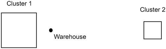
Figure 1.
Graphical illustration of the problem setting: Customers are distributed on the large high-density Cluster 1, closer to the warehouse, and the low-density Cluster 2, which is less convenient to serve.
Each customer request is characterized by a deadline, a volume, and a service time. Requests are served by a single vehicle featuring a limited volume capacity, measured in the same units as demand, and an average speed, which we use to estimate travel times given the distance and to check the maximum route duration constraint. Numerical values will be given in Section 7.
Since we deal with a single vehicle, we must plan one vehicle route per day, serving a subset of customer requests waiting in the queue. We first have to make a dispatching decision concerning the selection of the customers to be served today. This decision has an impact on service quality. Then, we have to solve a traveling salesperson problem (TSP) to minimize traveled distance (which also minimizes traveled time under our average speed hypothesis). We emphasize again that routing cannot be disregarded when making the dispatching decision, as we have not only a capacity constraint, which is easy to check [28], but also a route duration constraint. Nevertheless, when making the dispatching decision, we may consider a fast TSP heuristic, whereas when solving the TSP problem, we may apply a post-optimization strategy, if we wish. This consideration is crucial when dealing with the more realistic multi-vehicle VRP.
In order to formalize constraints, let us consider the set of customers dispatched for day t. If this set consists of n customers, the route may be considered a permutation of these n customers, with the addition of the deposit (say node 0 in the network) at the beginning and end of the route:
where is the node of the customer in position in the route. The deposit is in both position 0 and in the sequence. The total traveled distance in day t is then
where is the distance from node i to node j. The corresponding route duration is
where is the service time for each dispatched customer , and S is the average vehicle speed. We will assume that the main concern is to reduce the average traveled distance per day,
evaluated on a suitably long time horizon. This is significant in terms of environmental impact, but we also want to keep service quality under control.
In terms of individual customer service, we should consider the day on which customer k joins the queue, and the day on which its request is served. Then, for customer k with deadline , we should consider waiting time and tardiness (note that tardiness is zero for a customer that is served on time). Then, we may aggregate such quantities over customers and measure
- the average waiting time of customers;
- the percentage fraction of requests that are not served on time with respect to the deadline;
- the average tardiness over the subset of customers that are served late;
- the maximum tardiness (i.e., the worst case over the full simulated horizon).
We do not consider the average tardiness over all customers, since this statistic is not significant when most requests are served on time.
There is a tradeoff between these performance measures, as waiting for better opportunities to meet cluster 2 requests may reduce the traveled distance at the cost of an increased waiting time and possible deadline violations.
5. A PFA Approach
A PFA approach requires the definition of a mapping from states to actions. In an online problem, the decisions to make are relatively simple:
- Should we accept a request?
- At which point in the current route should the accepted request be inserted?
- Where should we position the vehicle if it is idle?
In our case, the decision concerns the subset of customers to be served today, which also involves solving a TSP subproblem (otherwise, we cannot check feasibility with respect to the route duration constraint). Sophisticated approaches based on neural networks are unsuitable, and a different mechanism must be devised. A simple framework is based on the following generic procedure:
- 1.
- Sort customer requests currently in the queue according to some criterion, which provides a priority list.
- 2.
- Start with an empty route (from the deposit to itself).
- 3.
- For each customer in the priority list, check if it can be feasibly inserted. This requires that
- its inclusion does not violate the capacity constraint (which is easy to check);
- its inclusion does not violate the route duration constraint (which we check quickly using a best insertion point heuristic). Note that the best insertion heuristic aims at minimizing the extra mileage incurred by growing the route. Since we assume that travel time is proportional to distance, this also aims at satisfying the route duration constraint.
If the customer can be inserted, grow the route by inserting it; otherwise, skip that customer (who is left in the queue for the next day). - 4.
- Repeat the previous step until the whole list has been scanned. Eliminate the dispatched requests from the queue.
- 5.
- If needed, run a high-quality TSP approach to post-optimize the resulting route.
The key is the definition of the sorting criterion. Naive benchmarks could rely on the time of arrival or the deadline, but since multiple requests share these quantities, a lexicographic approach based on multiple criteria should be adopted. To define a simple baseline for a comparison, we consider the following two naive policies:
- (first-in/first-out) sorts customers based on arrival time (increasing order), cluster (increasing), and requested volume (decreasing);
- (earliest deadline) uses deadline (increasing order), cluster (increasing), and requested volume (decreasing).
Note that time of arrival and deadline are related, but the induced ordering may differ, as the delivery time windows of two customers may not be the same, even if they join the queue on the same day. In the strategy, the time of arrival is the main criterion. A secondary criterion is the increasing order of the clusters, which means that we give priority to customers in high-density cluster 1 to avoid long trips to cluster 2, possibly for one customer. The last criterion is the requested volume, in decreasing order, which means that we try to fit customers that consume a large fraction of vehicle capacity in order to improve vehicle utilization. This is related to a well-known heuristic principle in bin packing. In , whose name is due to a classical dispatching rule for machine scheduling (earliest due date), the first criterion is based on urgency.
Rules like and are simplistic, but they are helpful benchmarks for more sophisticated policies. A better sorting strategy may be devised by taking advantage of the problem structure. As far as “inconvenient” requests from the low-density area are concerned, intuition suggests the following:
- Requests for which the deadline is today should be dispatched immediately, if possible, as we cannot wait further.
- If a request consumes a large fraction of vehicle capacity, there may be no point in waiting, as we might not be able to accommodate many other requests form the low-density cluster on the vehicle.
This suggests the definition of a trigger condition, such that requests from the low-density region should be placed at the top of the daily priority list if the condition is met. The trigger condition is related to the fraction of vehicle capacity required to meet all of the requests from cluster 2 in the current queue and to the time to deadline of the most urgent one. A similar approach, based on a threshold policy, is proposed, e.g., by [26].
Let us denote by the days to deadline (time slack) of the most urgent request from the low-density cluster in the current queue. Let us also denote by the threshold fraction, i.e., the minimum required capacity that triggers an immediate service event, as a function of . The idea is illustrated in Figure 2. Clearly , since on the deadline day we should serve the most urgent request, no matter what. If the queued requests from the low-density cluster are not urgent, their total required capacity should be large enough to justify the trip. As shown in Figure 2, if the fraction of truck capacity required by inconvenient customers is below a threshold, we are in the wait region; if the fraction of capacity is above the threshold, we are in the serve region. The threshold triggering the immediate service event should be an increasing function of , which measures the urgency of the most critical inconvenient customer.
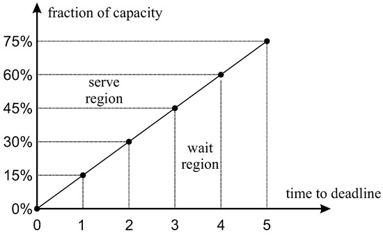
Figure 2.
Illustration of the trigger policy. For each time to deadline (of the most urgent customer in the low-density cluster), we specify a threshold capacity (total volume of requests from the low-density cluster) that separates the wait region from the immediate service region.
To be more precise, we consider a single-parameter trigger policy, corresponding to the slope of the line in Figure 2. The single parameter is a slope factor, which is the threshold capacity corresponding to the largest possible value of the time to deadline . In Figure 2, this is five days, and the slope factor is . Alternatively, rather than a straight line defined by its slope, we could assume a nonlinear curve and specify five different increasing thresholds (the threshold when there is an urgent or late delivery is always 0). When the trigger condition is met, the queued requests are sorted according to a lexicographic strategy, like in the and policies, but here the criteria are as follows:
| cluster (decreasing order), deadline (increasing order), | |||
| requested volume (decreasing order). |
Hence, in the immediate service region, priority is assigned to requests from cluster 2. If the trigger condition is not satisfied, the sorting criteria are:
so that priority is given to the high-density cluster 1.
| cluster (increasing order), deadline (increasing order), | |||
| requested volume (decreasing order), |
Policy parameters can be learned by simulation-based optimization, where the objective function may be a combination of the previously mentioned performance criteria or, as we do, just total traveled distance. As we have already pointed out, we try to avoid the difficult task of setting weights associated with conflicting objectives. The optimization task is clearly much easier for the single-parameter threshold policy. A natural question is whether this straightforward rule is satisfactory and robust, or the additional effort in optimizing multiple threshold parameters is justified.
6. A CFA Approach
A CFA approach may be devised by solving the dispatching problem as a prize-collecting traveling salesperson problem (PCTSP). We may associate a sort of profit measure with each customer in the current queue, which is related to its urgency, and maximize a combination of collected profit and traveled distance, subject to capacity and maximum route duration constraints.
To formulate the PCTSP model, we introduce two dummy nodes, an initial and a final one, corresponding to the deposit. Let N be the total number of nodes, where we assume that nodes 1 and N are the starting and terminal nodes of the path, i.e., the deposit. The model that we formulate is flow-based and is a variation of those described, for instance, in [19]. We introduce the following decision variables:
- , set to 1 if we visit node j after node i; 0 otherwise. We define such variables for , subject to the constraint .
- , set to 1 if we visit node i. We define such variables for , subject to the constraint .
- , which are auxiliary variables to eliminate subtours. Note that we use the classical Miller–Tucker–Zemlin formulation [29], which is not suitable for large-scale problems but is well-suited to our pilot case study. Other modeling approaches prevent subtours with an exponential number of inequalities (cuts), which are more efficient but require specific branch-and-cut solution approaches; see, e.g., [2].
We denote by the distance between nodes i and j, by S the average vehicle speed, by the item volume of request i, by the vehicle capacity, by the reward collected when visiting node i, and by the time needed to serve the corresponding customer. We set , .
An MILP model to maximize a weighted combination of profit and distance is the following:
The objective function (4) is a weighted combination of profit, with weight , and traveled distance, with weight . Constraint (5) makes sure that the path starts from node 1 and ends at node N. Equation (6) makes sure that each customer node is visited at most once and that flow is conserved. The node selection and arc flow variables are related by constraint (7). Constraints (8) and (9) are the capacity and route duration constraints, respectively. Equation (10) is the subtour elimination constraint, according to the Miller–Tucker–Zemlin formulation. It is well-known that such a formulation requires a polynomial number of constraints and does not require sophisticated branch-and-cut strategies. However, it leads to weak lower bounds. Nevertheless, it is a workable formulation for our pilot case study. In a real-life setting, we would apply a metaheuristic approach to solve a prize-collecting VRP [19]. We omit the definitional constraints on variables, as well as constraints fixing to 0 or 1 specific variables, which we have pointed out before. We should observe that the model formulation is suitable for asymmetric distances, less for symmetric distances, which we assume in the paper. To improve performance, we also add symmetry-breaking constraints like , which are redundant but may improve the performance of commercial MILP solvers.
A very critical point is the definition of profit and the choice of weights and . A pragmatic approach to circumvent a difficult choice of weight is based on a lexicographic strategy. We first solve the model settings and , which means that we just maximize profit. Note that tour length is partially kept under control by the route duration limit. This is used as a heuristic to select the dispatched customers. Then, we freeze the selection variables and solve a TSP problem, setting and . This tour re-optimization step often has a significant impact.
Regarding profits (priorities), a possible approach has been proposed by [17] based on the urgency of a customer and the measure of compatibility with other potential requests in the near future (assuming a fixed set of customers issuing random delivery requests), related to the savings obtained by serving certain customers together. However, we deal with a different setting, where the set of customers is not fixed but clustered. Instead of using that kind of a priori probabilistic information, we wish to check whether suitably parameterized priorities can be learned by simulation-based optimization.
One way to associate a profit with customer i is to rely on an exponential functional form,
where is the time to deadline of the customer i, which belongs to cluster , and , , and are suitably constrained parameters to be fine-tuned by simulation-based optimization. The selected form considers only urgency, leaving volume capacity and duration issues to the solution of the PCTSP problem. The priority of customer i exponentially increases as the time to deadline (slack) decreases. The exponential term is greater than 1 when we are late and . The parameter controls how fast the priority increases. The parameter induces a threshold effect, so that the profit can be negative if there is a large time slack, which implies that the customer will not be selected. The parameter may be used to differentiate the priorities, depending on the cluster k of customer i. One way to take advantage of this flexibility might be to induce an initially lower but faster growing priority for customers in cluster 2. Since priorities are relative, in our simple setting, we may fix , so that we have to fine-tune five parameters.
7. Computational Experiments
In carrying out computational experiments, we keep most problem features fixed to a baseline value and let the tightness of deadlines vary, as this is arguably the most relevant feature. We refrain from a large-scale experimentation, where results are often difficult to interpret, and focus on the impact of deadlines in order to carefully compare the PFA and CFA approaches within a multiobjective setting.
The basic geography of the problem is fixed as illustrated in Figure 1. The bottom-left (south-west) corner and the upper-right (north-east) corner have coordinates and , respectively (measured, e.g., in km). The coordinates of the deposit are , and the opposite corners for cluster 2 have coordinates and , respectively. Hence, the deposit is closer to the high-density, larger cluster. Customer locations are uniformly distributed within the clusters. Following other papers in the literature, such as [16], we assume plain Euclidean distances and Poisson arrivals.
The rates of request arrivals for the two clusters are and per day, respectively. Each delivery request is characterized by three attributes:
- 1.
- Time to deadline. If a request is received at the beginning of day t, the time window for delivery is from day t to day . We assume that the time to deadline is an integer number, uniformly distributed between given bounds that characterize the tightness of the time window. We use increasingly tight bounds on the time to deadline, in the ranges , , , and, finally, days for the tightest case. When the time to deadline is 0, it means that the request should be immediately serviced.
- 2.
- Volume, measured in the same units as vehicle capacity, is a real number uniformly distributed between 5 and 50.
- 3.
- Service time is a real number uniformly distributed between and 2 h.
There is a single vehicle, with a limited volume capacity of 250 (in the same units as demand). Vehicle speed is, on average, (we use an average speed, for the sake of simplicity, to estimate travel times given distance). The maximum route duration, including both travel and service times, is 10 h.
A back-of-the-envelope calculation can be run in order to check the tightness of capacity and duration constraints. Using the given Poisson rates, we see that the average time for service requirement per day is
whereas the average volume is
showing that the time constraint is expected to be more critical than volume for these values. Actually, the volume capacity constraint has an impact, too, since reducing volume capacity to, say, 200 has a significant effect on performance measures (we checked this in experiments that are not reported here for the sake of brevity).
The questions that we want to investigate are as follows:
- 1.
- What is the performance of a single-parameter trigger policy with respect to trivial FIFO and EDD benchmarks?
- 2.
- Is there any benefit in moving from a single- to a multi-parameter trigger policy?
- 3.
- Is there any benefit in additional TSP re-optimization in the trigger policy?
- 4.
- How do the PFA and CFA strategies compare?
The following four subsections address each question in turn. The comparison is carried out in terms of distance traveled and service quality, not in terms of computational effort. Needless to say, learning suitable parameters for the CFA approach is more demanding, as we have to solve multiple MILPs. However, the solution time for a single run is just a few seconds; hence, in terms of practical applicability, this is inconsequential.
7.1. Experiment 1
In the first experiment, we compared the performance of a single-parameter trigger policy against trivial FIFO and EDD benchmarks. To do so, we simulated a rather long time horizon of days to collect reliable statistics. The results are summarized in Table 1, Table 2, Table 3 and Table 4, which correspond to different degrees of deadline tightness. The trigger policy was run with four slope factors in the set . The last value in the set corresponds to a policy that requires a large capacity request from the inconvenient cluster to motivate an early trip there. Each table reports

Table 1.
PFA approaches: deadline range .
Table 2.
PFA approaches: deadline range .
Table 3.
PFA approaches: deadline range .
Table 4.
PFA approaches: deadline range .
- Av.Dist, the average distance traveled per day;
- Av.Wait, the average waiting time per customer;
- % Tard, the percentage fraction of requests that are serviced late;
- Av.Tard, the average tardiness over the subset of requests that are serviced late;
- Max.Tard, the maximum tardiness observed over the time horizon.
The stochastic process of arrival scenarios was carefully controlled, so that the arrival sequences were always the same across decision rules and the different degrees of deadline tightness. Therefore, the average traveled distance and waiting time did not change for the FIFO and EDD policies, as only the deadlines for each request were changed, uniformly for each customer, across the four tables.
Table 1, related to the case of loose deadlines, points out a slight tradeoff in terms of waiting time and missed deadlines between and , which is expected. A suitably parameterized policy is able to considerably reduce traveled distance while improving service level. Note that numbers were rounded to two decimals, so when we read , the actual number need not be exactly zero. In this setting, the fraction of late services is less than 0.1%, but tardiness may be occasionally significant. Table 2, Table 3 and Table 4 show that when deadlines get tighter, the ability of the policy to reduce traveled distance is impaired, as there is less flexibility in waiting to serve inconvenient customers. Nevertheless, the policy dominates the naive benchmarks in terms of service quality as well. Again, even though the average tardiness is not large, the worst-case value may be large, as shown by the maximum tardiness column. This can be explained by an occasional congestion effect due to arrival variability and the possible combination of large capacity and time requirements (keep in mind that we simulated a very long time horizon, so a relatively extreme congestion event may be observed). This suggests the opportunity of a refinement of the policies, which should behave differently when tardiness exceeds one or two days. However, it is quite likely that, in real life, these cases would be dealt with by emergency actions like overtime or by resorting to a third-party operator.
7.2. Experiment 2
Experiment 1 shows that the choice of the slope factor in the single-factor policy has a significant impact on performance. The optimization of this single factor is easy to accomplish, but we should ask whether the flexibility that we may obtain by using multiple thresholds is worth the additional effort. In this case, the increased computational requirements of the optimization process do not allow to use a very long time horizon for simulation-based optimization. We tuned parameters on a shorter horizon of 5000 days but compared performance on the long out-of-sample horizon of days. The objective function for simulation-based optimization is the average traveled distance but, as before, we report other measures related to service quality.
Optimizing the single-parameter trigger policy is easy, as it requires minimizing a function of a single variable, the slope factor, which we accomplished using the function of MATLAB R2024a. The only constraint is that the slope factor must be in the range . Optimizing multiple thresholds is a bit more challenging, especially when the maximum time to deadline is relatively large. In the case of Figure 2, there are five variables (the threshold for is 0). After an initial unsatisfactory experience with pattern search, we resorted to particle swarm optimization, as implemented by the function of MATLAB. The number of particles in the swarm was set to a large value, 150, and the procedure was stopped after stalling for 20 iterations. The computational effort was reduced by taking advantage of parallel computing in MATLAB. However, as we pointed out before, this is not necessarily relevant for practical purposes, as learning decision rules occurs offline and their online application is fast. Since does not allow for constraints other than lower and upper bounds, to ensure that thresholds are increasing, we optimized with respect to non-negative and bounded increments in the thresholds.
The results are reported in Table 5, which provides the relevant performance measures for and threshold policies (column ), for the four different cases of time window tightness (column ). A cursory look at the results shows that, indeed, there is some advantage in optimizing multiple thresholds, but it is not so significant. Moreover, in the last case, corresponding to the tightest delivery time windows, there is no difference in performance. This is not so surprising, actually, since in this setting, there are only two threshold levels to be optimized in the rule.
Table 5.
Performance measures for optimized trigger policies.
Some additional insight may be gained by looking at the optimized parameters, reported in Table 6, rounded to three decimal digits. In the case of loose deadlines (first row), we notice fairly compatible parameters, in the sense that the thresholds for the largest time to deadline, and , are similar, even though the increments for the multiple thresholds case do not look particularly constant. A more interesting pattern emerges in the other three cases, as there is an immediate increment in the thresholds when moving from time to deadline to , whereas the successive thresholds do not increase much, or stay even constant. This suggests that the relevant parameter is the threshold for , and that when the the single threshold is large, it induces such a threshold also in the single-parameter case. A possible explanation is that, for the analyzed setting, we should wait a bit more before serving the difficult cluster, and this is arguably due to the fact that there is enough vehicle capacity for doing so, due to the low arrival rate in the low-density region.
Table 6.
Optimal parameters for optimized trigger policies.
A parsimonious parameterization could be adopted, where we set two thresholds for time to deadline and and then interpolate linearly for the intermediate values. We refrained from doing so, due to the very marginal improvement with respect to the simpler policy, which is the only one used in the remaining experiments.
It is also important to notice that we were optimizing with respect to the average traveled distance, even though we also measured other performance measures, in order to avoid issues with weight setting in a multiobjective framework (tracing efficient frontiers is probably not practical in our dynamic setting). In an early experiment, not reported here, we did not constrain the initial threshold to 0. This resulted in a relatively large initial threshold, a reduced traveled distance, and a very poor service quality. By adding the reasonable constraint , we were able to achieve much more satisfactory results. This suggests that a simple policy function, with a parsimonious set of parameters, may be used to control multiple measures in a pragmatic way, even though we steered away from formally trading off multiple objectives.
7.3. Experiment 3
In this experiment, we checked the reduction in average traveled distance that could be achieved in the single-parameter trigger policy if we post-optimized the route by solving the TSP subproblem exactly. This was achieved using the MATLAB MILP solver on a TSP model. We do not report the model, which is essentially the same as Section 6, with suitable simplifications. In Table 7, we report the average traveled distance without and with post-optimization, and the percentage reduction, in the four tightness settings. The other performance measures were unaffected by post-optimization. In this experiment, we used a single-parameter trigger policy, with the optimal settings of Table 6. Even though the additional effort to solve the TSP subproblem (by an inefficient model formulation) is negligible for a single day, it does have an impact on a long horizon. Hence, we report a simulation with a limited time horizon of 1500 days.
Table 7.
Improvements obtained by TSP post-optimization for the single-threshold policy.
Table 7 shows that the percentage reduction when post-optimizing the TSP tour is less than 1%. This is not particularly surprising, since the time constraint was tight and the number of customer visits per tour was small, so that a simple insertion heuristic performed reasonably well (it is also used, e.g., in the online context of [16]). It might be argued that the point is moot and that it is always worth improving the solution, if this implies a negligible increase in computational effort. However, the rationale behind this experiment should be appreciated in a more general context, where we may wish to optimize multiple thresholds, which would be computationally much more expensive if we always post-optimize, or when we want to use the trigger policy as a baseline policy within lookahead strategies, like myopic rollout or Monte Carlo tree search. In such cases, we would have to run the TSP solver multiple times even for the actual daily decision, so that the effort may become significant. Hence, it is useful to know that we may speed up computation by reserving the exact TSP solution for a limited post-optimization phase after the dispatching decision has been made.
7.4. Experiment 4
In this last experiment, we wanted to compare the CFA approach against the simple single-threshold policy. In order to get a feeling for the adequacy and effectiveness of the proposed functional form of Equation (11), we considered an exploratory run for the case of a tightness range of . The five parameters were optimized by pattern search, with upper bounds provided by . Due to the computational effort involved, the time horizon for each simulation was limited to 100 days, and the number of function evaluations (which require a simulation run, solving the PCTSP each day) was limited to 100. The resulting parameter setting is
We cannot claim that this is the optimal setting, but we may observe that was set to its upper bound (given the functional form, this parameter cannot take values larger than 1, the value attained by the exponential function at point 0, otherwise the profit will always be negative and no customer will ever be selected). This had the effect of delaying customers in cluster 2 considerably. To check the actual behavior, we ran the CFA approach with this parameter setting on an out-of-sample horizon of 1500 days, obtaining the following performance measures:
A comparison with Table 5 shows that these are definitely poor results. An explanation is that, in order to better pool delivery requests and reduce traveled distance, the resulting dispatching procedure delays deliveries too much. This suggests to avoid negative profits altogether and to eliminate the parameters from the functional form. Hence, we tried optimizing the remaining three parameters with the following lower and upper bounds:
Note that we set a lower bound for to avoid assigning very low priorities (possibly 0) to inconvenient customers, which would never be visited in order to reduce distance. We used particle swarm optimization, as provided by MATLAB, with a swarm size of 20, stopping after 10 stalling iterations. The time horizon in the optimization step was 100 days, whereas the out-of-sample testing was carried out on a time horizon of 1500 days. We should note that, since for each simulated day we had to build and solve an MILP model, even though a small one, the resulting computational effort is non-negligible. Using a powerful workstation with eight cores, the elapsed time for simulation-based optimization was more than 6 h in the worst case.
The results are shown in Table 8, and a comparison with those of Table 5 suggests that this is not a competitive approach. Except for the average traveled distance in the last row, corresponding to the tightest deadline setting, the results look worse than those obtained using the simpler trigger policy. Such a disappointing performance might be partially attributed to an obvious weakness in the approach: The MILP model aims at maximizing profits, but the simulation-based procedure aims at reducing traveled distance, with a possible detrimental effect on the other measures. It would be possible to use a multiobjective approach to fine-tune parameters. However, this would require, in turn, specifying priorities among the objectives, which is what we would like to avoid. We should note that a simpler PFA approach does a better job at that, without many complications.
Table 8.
Performance measures and parameters for the CFA approach.
It is instructive to look at the values of the fine-tuned parameters. In the first and third rows, we have and forced, respectively, to the lower and upper bounds. This has the effect of delaying service to the inconvenient cluster, in the hope of reducing traveled distance. On the one hand, this is not what we should do; on the other one, this approach does not look particularly successful in this respect either, probably because the customer selection by the MILP model for PCTSP relies on a lexicographic approach. It may also be argued that we should spend more computational resources in simulation-based optimization, or adopt a better approach than particle swarm. The fact remains that this CFA approach seems much more difficult to apply than a PFA approach, unless we are ready to commit to weights and formulate a single objective accounting for all problem dimensions.
8. From TSP to VRP
The computational experiments that we have reported are a necessary methodological step but, in order to apply the proposed approaches to a more realistic setting, we must devise possible strategies to generalize them to from a single-vehicle, capacitated TSP problem to the case of a multi-vehicle VRP. From this viewpoint, the CFA approach has an advantage in terms of flexibility, as the extension to a prize-collecting VRP is natural and metaheuristics are available. However, the experimental evidence suggests pursuing an extension of the PFA approach. We should also mention that, in the related but different setting of [30], a parameterized policy-based strategy is applied as well. Another interesting observation is that the parameterized policy is computationally cheaper, which allows for its inclusion in lookahead policies. See, e.g., [5] for a discussion of lookahead in stochastic inventory routing.
A clear disadvantage of the proposed trigger policy is that it is not obvious how to extend it to the VRP case. We recall that old-style classical constructive heuristics for CVRPs may be classified as sequential and parallel. In the sequential approach, a single route is grown at a time, and such a sequential strategy fits well with the proposed trigger policy, especially if we consider the association of a vehicle to a single inconvenient cluster at a time. It may well be argued that a sequential approach may turn out to be myopic and result in non-ideal routes. Nevertheless, the policy is not really used to find routes but just to solve the dispatching subproblems. After selecting the subset of customers for the day, we can post-optimize the routes using any standard CVRP heuristic.
Another potential improvement might be obtained by opportunistically inserting additional customers, which were not included by the dispatcher, from the convenient, high-density cluster in order to preserve reactive capacity for the following days, without significantly increasing route lengths. In fact, this is actually an approach taken in the real retail chain that motivated this paper. In fact, a relevant feature of the proposed approach is its simplicity, which is important in terms of end-user acceptance and potential integration within a more general framework.
9. Conclusions and Further Research Opportunities
We investigated simple decision policies for an offline, dynamic, and multiperiod capacitated TSP under uncertainty. The problem features were motivated by a real-life VRP, where there is spatial heterogeneity in the distribution of customers. To the best of our knowledge, the specific combination of features of this problem has not been considered in the rich and growing literature on dynamic and stochastic VRPs.
In order to gather useful insights to be applied on the full-scale problem, we considered the single-vehicle case. This preliminary step is fundamental for comparing simple ADP policies, based on policy function and cost function approximations, and to check if multiple and conflicting objectives may be simultaneously kept under control, without resorting to multiobjective strategies, whose practical applicability in a dynamic and uncertain context may be problematic.
The reported computational experiments showed that a simple trigger policy based on capacity thresholds can attain satisfactory results with quite limited computational effort. There is room for improvement, but the result is useful, as the resulting policy may be used as a baseline policy that can be leveraged in more sophisticated ADP strategies incorporating lookahead, such as myopic rollout or Monte Carlo tree search, which have proven their value when dealing with very challenging decision-making problems under sequential uncertainty.
The cost function approach that we investigated did not perform well. It would certainly be possible to improve its behavior by resorting to multiobjective optimization; however, apart from the well-known difficulties in selecting weights capturing managerial tradeoffs, the resulting approach is computationally more demanding and less suited to be integrated with lookahead strategies.
There are two next steps that we are going to pursue in further investigations:
- 1.
- On the one hand, we want to consider possible improvements when congestion occurs and customer service degrades. The trigger conditions that we analyzed refer only to volume capacity. It is also natural to wonder if improvements could result by considering time capacity, which is much more challenging since checking the exact route duration requires solving a routing problem. Nevertheless, we may try to anticipate the impact of dispatching decisions on routing, using either simple and old-style routing concepts, like extra-mileage, or more recent machine learning strategies [31].
- 2.
- On the other hand, we will consider the application of trigger policies in the more challenging and realistic multi-vehicle setting, along the lines described in Section 8.
Author Contributions
Conceptualization, S.M., P.B. and A.M.; methodology, S.M. and P.B.; software, P.B.; validation, S.M., P.B. and A.M.; writing—original draft preparation, S.M. and P.B.; writing—review and editing, S.M., P.B. and A.M. All authors have read and agreed to the published version of the manuscript.
Funding
This research received no external funding.
Data Availability Statement
Data sharing is not applicable—no new data were generated.
Acknowledgments
P. Brandimarte is grateful to his colleague, G. Zotteri, for pointing out this class of VRPs based on his real-life experience.
Conflicts of Interest
Authors Subei Mutailifu and Aili Maimaiti are employed by the company Xinjiang Academy of Transportation Sciences Co., Ltd. The remaining author declares that the research was conducted in the absence of any commercial or financial relationships that could be construed as a potential conflict of interest.
References
- Golden, B.; Raghavan, S.; Wasil, E.A. (Eds.) The Vehicle Routing Problem: Latest Advances and New Challenges; Springer: Berlin/Heidelberg, Germany, 2008. [Google Scholar]
- Toth, P.; Vigo, D. (Eds.) Vehicle Routing: Problems, Methods, and Applications, 2nd ed.; Society for Industrial and Applied Mathematics: Philadelphia, PA, USA, 2015. [Google Scholar]
- Archetti, C.; Jabali, O.; Speranza, M.G. Multi-period vehicle routing problem with due dates. Comput. Oper. Res. 2015, 61, 122–134. [Google Scholar] [CrossRef]
- Psaraftis, H.N.; Wen, M.; Kontovas, C.A. Dynamic vehicle routing problems: Three decades and counting. Networks 2016, 67, 3–31. [Google Scholar] [CrossRef]
- Cuellar-Usaquén, D.; Ulmer, M.W.; Gomez, C.; Álvarez-Martínez, D. Adaptive stochastic lokkahead policies for dynamic multi-period purchasing and inventory routing. Eur. J. Oper. Res. 2024, 318, 1028–1041. [Google Scholar] [CrossRef]
- Brandimarte, P. From Shortest Paths to Reinforcement Learning: A MATLAB-Based Introduction to Dynamic Programming; Springer: Berlin/Heidelberg, Germany, 2021. [Google Scholar]
- Powell, W.B. Approximate Dynamic Programming: Solving the Curses of Dimensionality, 2nd ed.; Wiley: Hoboken, NJ, USA, 2011. [Google Scholar]
- Powell, W.B. Clearing the jungle of stochastic optimization. In INFORMS TutORials: Bridging Data and Decisions; Institute for Operations Research and the Management Sciences: Catonsville, MD, USA, 2014; pp. 109–137. [Google Scholar]
- Geist, M.; Pietquin, O. Algorithmic survey of parametric value function approximation. IEEE Trans. Neural Netw. Learn. Syst. 2013, 24, 845–867. [Google Scholar] [CrossRef] [PubMed]
- Browne, C.B.; Powley, E.; Whitehouse, D.; Lucas, S.M.; Cowling, P.I.; Rohlfshagen, P.; Tavener, S.; Perez, D.; Samothrakis, S.; Colton, S. A survey of Monte Carlo tree search methods. IEEE Trans. Comput. Intell. AI Games 2012, 4, 1–43. [Google Scholar] [CrossRef]
- Bertsekas, D.P. Rollout, Policy Iteration, and Distributed Reinforcement Learning; Athena Scientific: Nashua, NH, USA, 2020. [Google Scholar]
- Powell, W.B. Reinforcement Learning and Stochastic Optimization: A Unified Framework for Sequential Decisions; Wiley: Hoboken, NJ, USA, 2019. [Google Scholar]
- Bogyrbayeva, A.; Meraliyev, M.; Mustakhov, T.; Dauletbayev, B. Machine learning to solve vehicle routing problems: A survey. IEEE Trans. Intell. Transp. Syst. 2024, 25, 4754–4772. [Google Scholar] [CrossRef]
- Ulmer, M.W. Approximate Dynamic Programming for Dynamic Vehicle Routing; Springer: Berlin/Heidelberg, Germany, 2017. [Google Scholar]
- Powell, W.B.; Simao, H.P.; Bouzaiene-Ayari, B. Approximate dynamic programming in transportation and logistics: A unified framework. EURO J. Transp. Logist. 2012, 1, 237–284. [Google Scholar] [CrossRef]
- Ulmer, M.W.; Soeffker, N.; Mattfeld, D.C. Value function approximation for dynamic multi-period vehicle routing. Eur. J. Oper. Res. 2018, 269, 883–899. [Google Scholar] [CrossRef]
- Albareda-Sambola, M.; Fernández, E.; Laporte, G. The dynamic multiperiod vehicle routing problem with probabilistic information. Comput. Oper. Res. 2014, 48, 31–39. [Google Scholar] [CrossRef]
- Ulmer, M.W.; Thomas, B.W. Meso-parametric value function approximation for dynamic customer acceptances in delivery routing. Eur. J. Oper. Res. 2020, 285, 183–195. [Google Scholar] [CrossRef]
- Vansteenwegen, P.; Gunawan, A. Orienteering Problems: Models and Algorithms for Vehicle Routing Problems with Profits; Springer: Berlin/Heidelberg, Germany, 2019. [Google Scholar]
- Bosse, A.; Ulmer, M.W.; Manni, E.; Mattfeld, D.C. Dynamic priority rules for combining on-demand passenger transportation and transportation of goods. Eur. J. Oper. Res. 2023, 309, 399–408. [Google Scholar] [CrossRef]
- Secomandi, N. A rollout policy for the vehicle routing problem with stochastic demands. Oper. Res. 2001, 49, 796–802. [Google Scholar] [CrossRef]
- Goodson, J.C. Rollout policies for dynamic solutions to the multivehicle routing problem with stochastic demand and duration limits. Oper. Res. 2013, 61, 138–154. [Google Scholar] [CrossRef]
- Heitmann, R.J.O.; Soeffker, N.; Ulmer, M.W.; Mattfeld, D.C. Combining value function approximation and multiple scenario approach for the effective management of ride-hailing services. EURO J. Transp. Logist. 2023, 12, 100104. [Google Scholar] [CrossRef]
- Ulmer, M.W. Horizontal combinations of online and offline approximate dynamic programming for stochastic dynamic vehicle routing. Cent. Eur. J. Oper. Res. 2020, 28, 279–308. [Google Scholar] [CrossRef]
- Ulmer, M.W.; Goodson, J.C.; Mattfeld, D.C.; Hennig, M. Offline-online approximate dynamic programming for dynamic vehicle routing with stochastic requests. Transp. Sci. 2019, 53, 185–202. [Google Scholar] [CrossRef]
- Gautam, N.; Geunes, J. Analysis of real-time order fulfillment policies: When to dispatch a batch? Serv. Sci. 2023, 16, 85–106. [Google Scholar] [CrossRef]
- Jozefowiez, N.; Semet, F.; Talbi, E.G. Multi-objective vehicle routing problems. Eur. J. Oper. Res. 2008, 189, 293–309. [Google Scholar] [CrossRef]
- Fisher, M.L.; Jaikumar, R. A generalized assignment heuristic for vehicle routing. Networks 1981, 11, 109–124. [Google Scholar] [CrossRef]
- Miller, C.; Zemlin, R.; Tucker, A. Integer programming formulation of traveling salesman problems. J. ACM (JACM) 1960, 7, 326–329. [Google Scholar] [CrossRef]
- Stein, J.; Hildebrandt, F.D.; Ulmer, M.W.; Thomas, B.W. Learning state-dependent policy parametrizations for dynamic technician routing with rework. Transp. Sci. 2025; ahead of print. [Google Scholar] [CrossRef]
- Varol, T.; Özener, O.; Albey, E. Neural network estimators for optimal tour lengths of traveling salesperson problem instances with arbitrary node distributions. Transp. Sci. 2023, 58, 45–66. [Google Scholar] [CrossRef]
Disclaimer/Publisher’s Note: The statements, opinions and data contained in all publications are solely those of the individual author(s) and contributor(s) and not of MDPI and/or the editor(s). MDPI and/or the editor(s) disclaim responsibility for any injury to people or property resulting from any ideas, methods, instructions or products referred to in the content. |
© 2025 by the authors. Licensee MDPI, Basel, Switzerland. This article is an open access article distributed under the terms and conditions of the Creative Commons Attribution (CC BY) license (https://creativecommons.org/licenses/by/4.0/).