
Modular Coordination of Vehicle Routing and Bin Packing Problems in Last Mile Logistics


Abstract
1. Introduction
1.1. The Vehicle Routing Problem
1.2. The 3D Bin Packing Problem
1.3. Integration of CVRP and 3D-BPP
1.4. Paper Contributions
- (1)
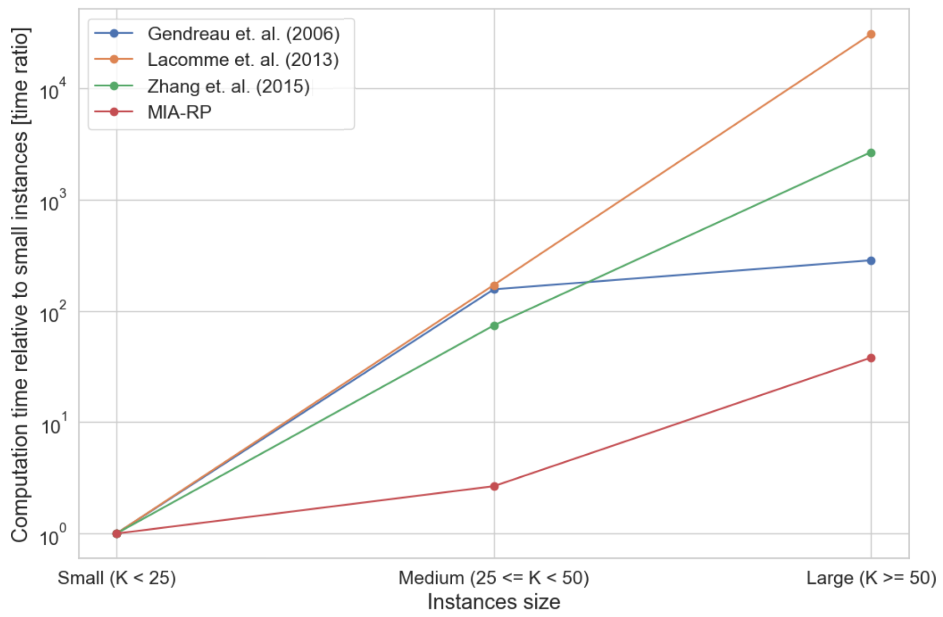
- Modular iterative algorithm for integrated VRP and BPP optimization of commensurate suboptimality but of significant improvement in execution speed when validated and compared to state-of-art approaches and ideal benchmark from [36],
- (2)
- Real case study benchmark and validation of the proposed algorithm, proving significant route savings of 14.48% on average.
2. Capacitated Vehicle Routing Problem Formulation
2.1. Initial Solution
| Algorithm 1: Randomized Constrained Clarke–Wright |
|
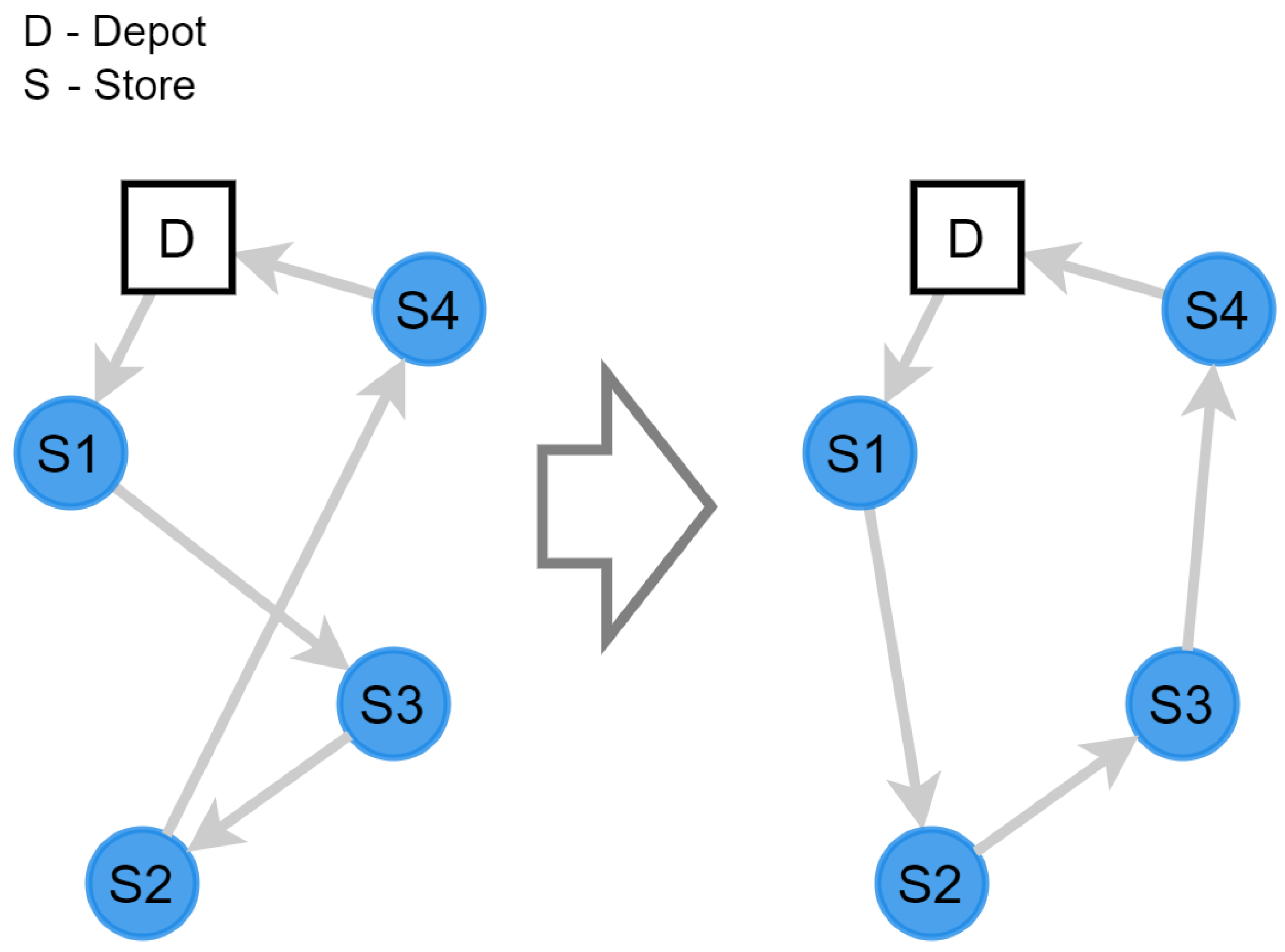
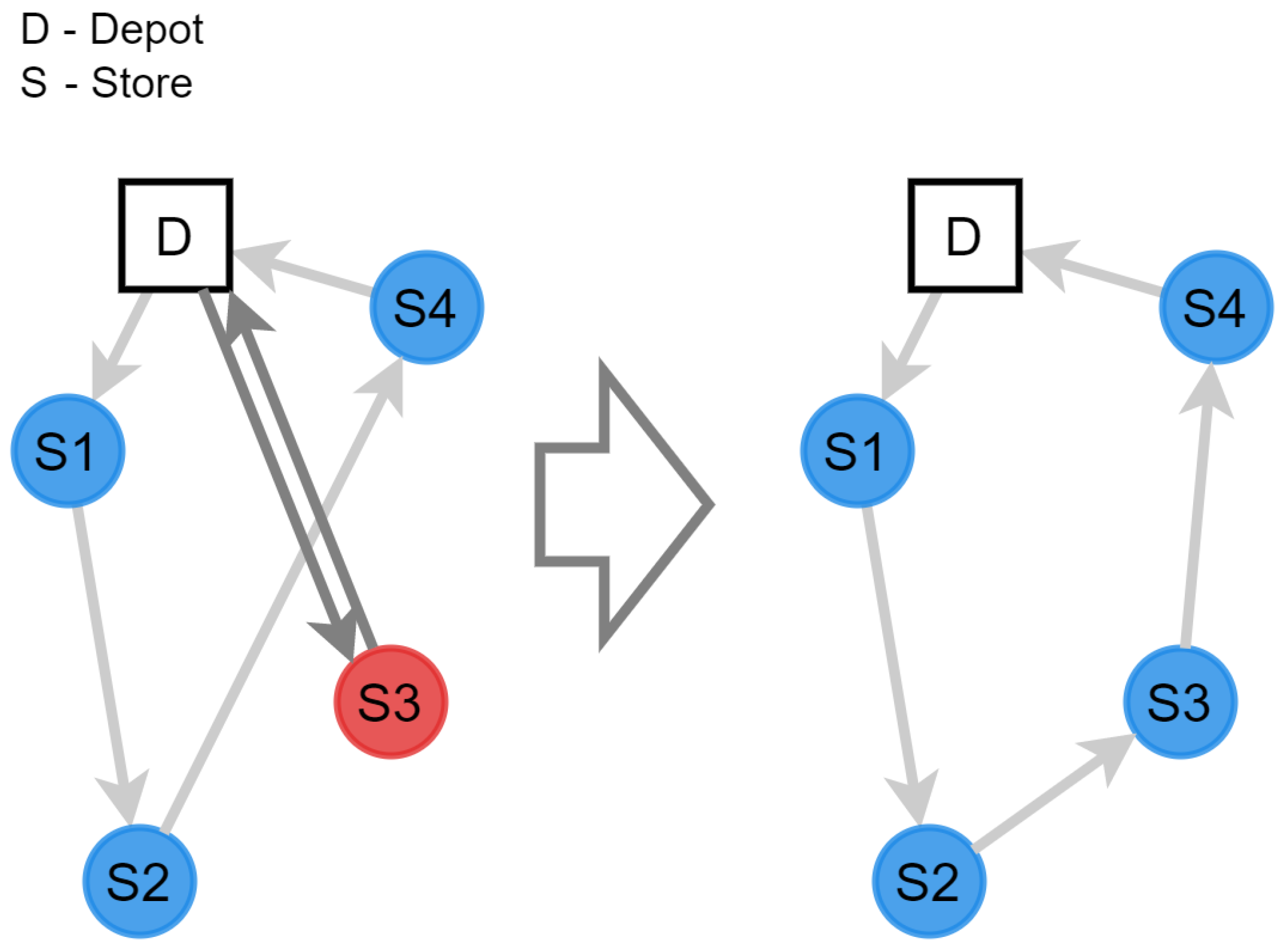
2.2. Local Search
2.3. Adaptive Memory Procedure
| Algorithm 2: Adaptive Memory Procedure |
|
3. 3D Bin Packing Problem Formulation
3.1. Genetic Algorithm
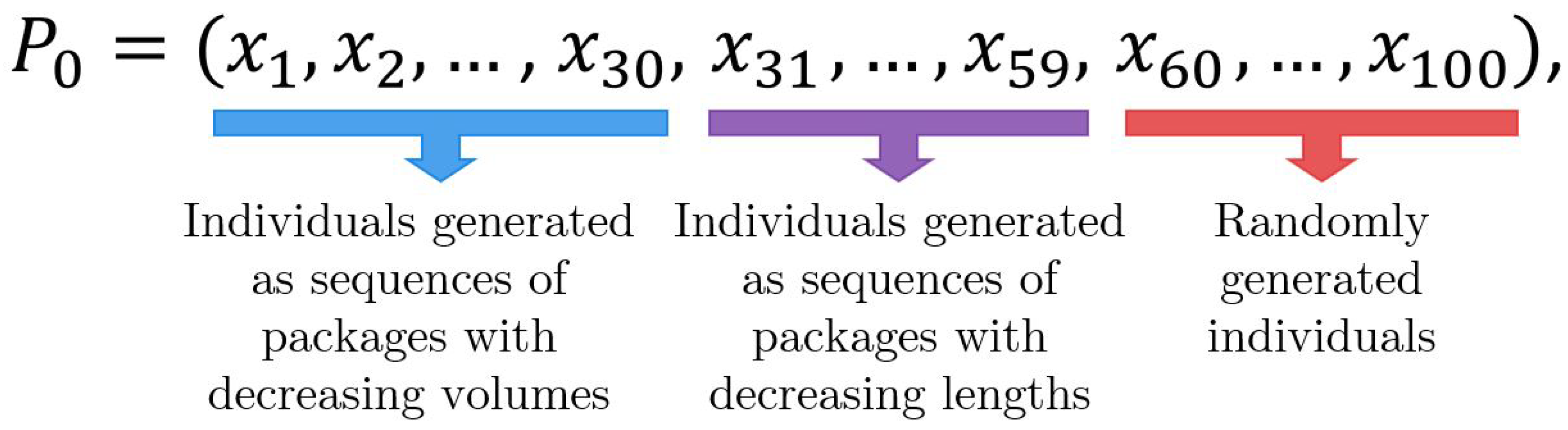
3.1.1. Initialization
3.1.2. Selection
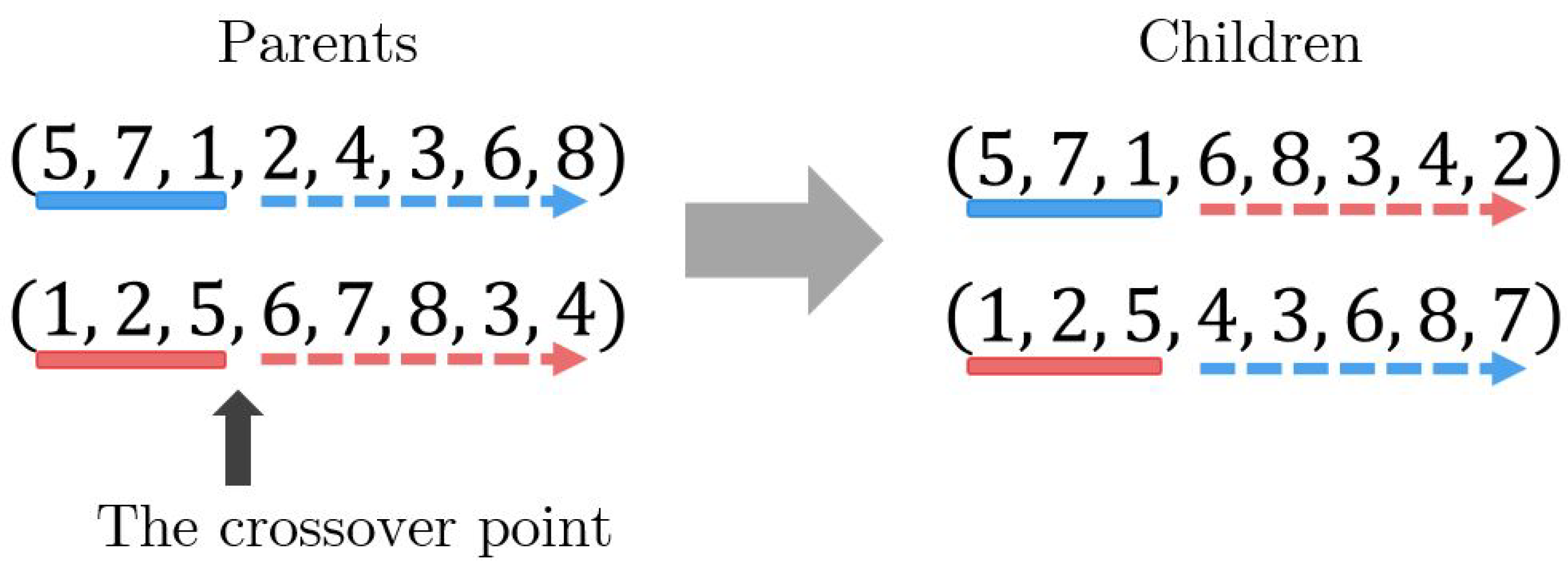
3.1.3. Crossover
3.1.4. Mutation
3.1.5. Lifo-Correction
3.1.6. Stopping Criteria
4. Coordination of Routing and Packing
- each customer is visited exactly once,
- each vehicle route starts and ends at the depot,
- distances between locations are known,
- all vehicles are available at the beginning with weight and volume constraints,
- the cargo consists of cuboid 3D packages with defined characteristics (shape, volume, weight, fragility, support, rotation, and rotation permissibility)
- unloading follows the LIFO principle where necessary.
- Optimization of delivery routes by resolving the associated CVRP from (3) s.t. (1) and (2) and (4)–(7).
- Validation of CVRP results by solving 3D-BPP for each individual vehicle from (9) s.t. (10)–(27), also considering shape, weight, fragility, support, rotation, and permissibility of rotation from [22].
- Increasing the virtual volumes of all packages associated with vehicles that provide infeasible solutions.
4.1. Optimization of Delivery Routes
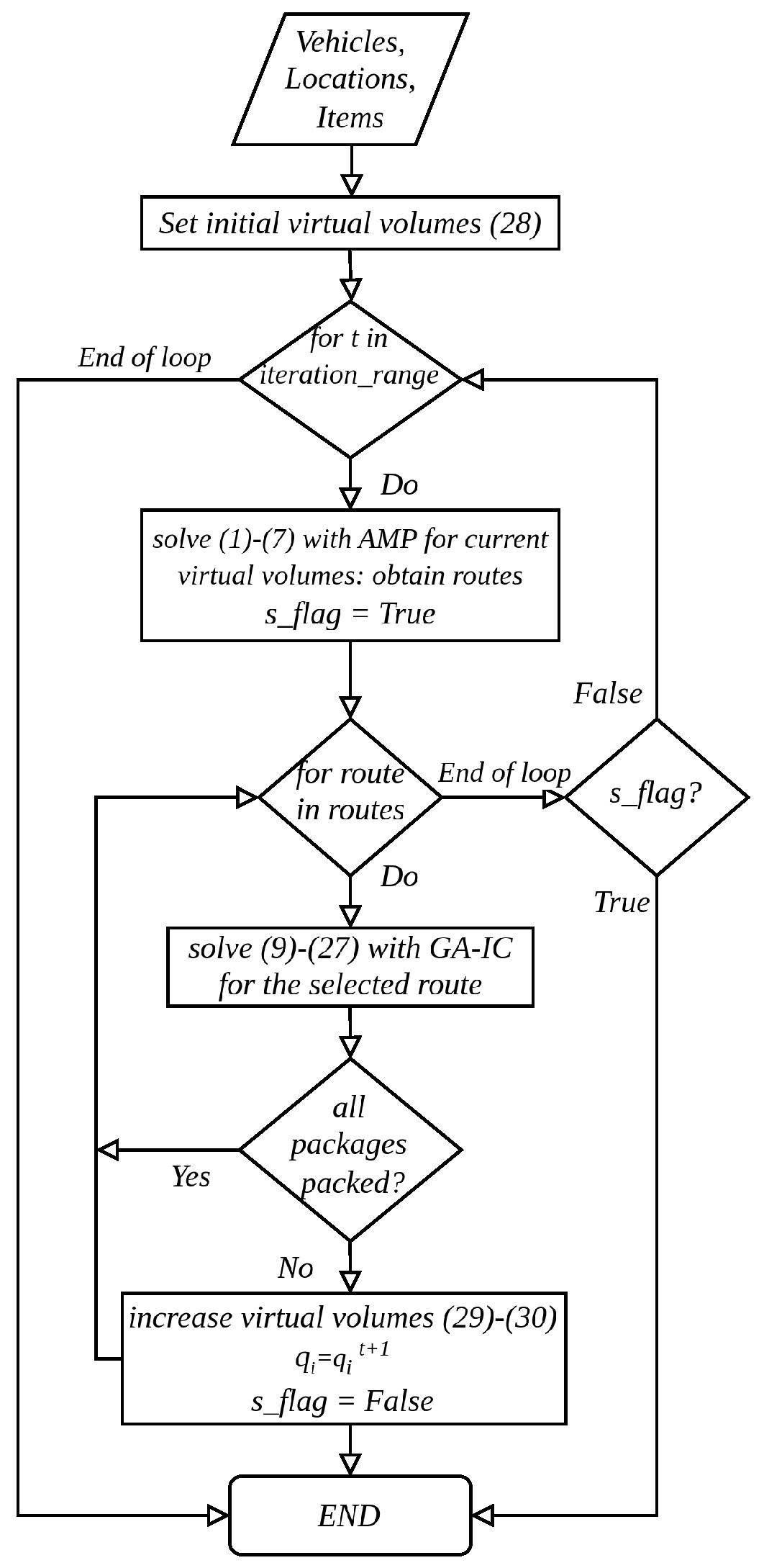
| Algorithm 3: MIA-RP |
|
4.2. Validation of VRP Results by Solving Packing Problems
4.3. Increasing the Virtual Volumes of All Packages Associated with Vehicles with Unfeasible Packing
4.4. Stopping Criteria
5. Computational Experiments
5.1. Experiments on Instances from the Literature
5.2. Experiments on Real-World Instances
5.3. Practical Implications, Limitations, and Future Work
6. Conclusions
Supplementary Materials
Author Contributions
Funding
Data Availability Statement
Acknowledgments
Conflicts of Interest
References
- Transport in the European Union—Current Trends and Issues. 2024. Available online: https://transport.ec.europa.eu/news-events/news/new-eu-transport-report-current-trends-and-issues-2024-06-27_en (accessed on 25 May 2025).
- Seyyedhasani, H.; Dvorak, J.S. Using the Vehicle Routing Problem to reduce field completion times with multiple machines. Comput. Electron. Agric. 2017, 134, 142–150. [Google Scholar] [CrossRef]
- Zhang, Z.; Wei, L.; Lim, A. An evolutionary local search for the capacitated vehicle routing problem minimizing fuel consumption under three-dimensional loading constraints. Transp. Res. Part B Methodol. 2015, 82, 20–35. [Google Scholar] [CrossRef]
- Nolz, P.C.; Absi, N.; Feillet, D.; Seragiotto, C. The consistent electric-Vehicle routing problem with backhauls and charging management. Eur. J. Oper. Res. 2022, 302, 700–716. [Google Scholar] [CrossRef]
- Laporte, H.; Mercure, G.L.; Nobert, Y. An exact algorithm for the asymmetrical capacitated vehicle routing problem. Networks 1986, 16, 33–46. [Google Scholar] [CrossRef]
- Rochat, Y.; Taillard, E. Probabilistic diversification and intensification in local search for vehicle routing. J. Heuristics 1995, 1, 147–167. [Google Scholar] [CrossRef]
- Gmira, M.; Gendreau, M.; Lodi, A.; Potvin, J.Y. Tabu search for the time-dependent vehicle routing problem with time windows on a road network. Eur. J. Oper. Res. 2021, 288, 129–140. [Google Scholar] [CrossRef]
- Sze, J.F.; Salhi, S.; Wassan, N. An adaptive variable neighbourhood search approach for the dynamic vehicle routing problem. Comput. Oper. Res. 2024, 164, 106531. [Google Scholar] [CrossRef]
- Saker, A.; Eltawil, A.; Ali, I. Adaptive Large Neighborhood Search Metaheuristic for the Capacitated Vehicle Routing Problem with Parcel Lockers. Logistics 2023, 7, 72. [Google Scholar] [CrossRef]
- Chen, C.M.; Lv, S.; Ning, J.; Wu, J.M.T. A Genetic Algorithm for the Waitable Time-Varying Multi-Depot Green Vehicle Routing Problem. Symmetry 2023, 15, 124. [Google Scholar] [CrossRef]
- Teng, Y.; Chen, J.; Zhang, S.; Wang, J.; Zhang, Z. Solving dynamic vehicle routing problem with time windows by ant colony system with bipartite graph matching. Egypt. Inform. J. 2024, 25, 100421. [Google Scholar] [CrossRef]
- Vinyals, O.; Fortunato, M.; Jaitly, N. Pointer networks. Adv. Neural Inf. Process. Syst. 2015, 28, 2692–2700. [Google Scholar]
- Pan, W.; Liu, S.Q. Deep reinforcement learning for the dynamic and uncertain vehicle routing problem. Appl. Intell. 2023, 53, 405–422. [Google Scholar] [CrossRef]
- Dulac-Arnold, G.; Levine, N.; Mankowitz, D.J.; Li, J.; Paduraru, C.; Gowal, S.; Hester, T. Challenges of real-world reinforcement learning: Defnitions, benchmarks and analysis. Mach. Learn. 2021, 110, 2419–2468. [Google Scholar] [CrossRef]
- Christofides, N. The vehicle routing problem. In Combinatorial Optimization; Christofides, N., Mingozzi, A., Toth, P., Sandi, C., Eds.; Wiley: Chichester, UK, 1979; pp. 315–338. [Google Scholar]
- Tarantilis, C.D. Solving the vehicle routing problem with adaptive memory programming methodology. Comput. Oper. Res. 2005, 32, 2309–2327. [Google Scholar] [CrossRef]
- Li, X.; Leung, S.C.H.; Tian, P. A multistart adaptive memory-based tabu search algorithm for the heterogeneous fixed fleet open vehicle routing problem. Expert Syst. Appl. 2012, 39, 365–374. [Google Scholar] [CrossRef]
- Simeonova, L.; Wassan, N.; Salhi, S.; Nagy, G. The heterogeneous fleet vehicle routing problem with light loads and overtime: Formulation and population variable neighbourhood search with adaptive memory. Expert Syst. Appl. 2018, 114, 183–195. [Google Scholar] [CrossRef]
- Nikolopoulou, A.I.; Repoussis, P.P.; Tarantilis, C.D.; Zachariadis, E.E. Adaptive memory programming for the many-to-many vehicle routing problem with cross-docking. Oper. Res. 2019, 19, 1–38. [Google Scholar] [CrossRef]
- Morais, V.W.; Mateus, G.R.; Noronha, T.F. Iterated local search heuristics for the Vehicle Routing Problem with Cross-Docking. Expert Syst. Appl. 2014, 41, 7495–7506. [Google Scholar] [CrossRef]
- Paquay, C.; Schyns, M.; Limbourg, S. A mixed integer programming formulation for the three-dimensional bin packing problem deriving from an air cargo application. Int. Trans. Oper. Res. 2016, 23, 187–213. [Google Scholar] [CrossRef]
- Paquay, C.; Schyns, M.; Limbourg, S. A tailored two-phase constructive heuristic for the three-dimensional Multiple Bin Size Bin Packing Problem with transportation constraints. Eur. J. Oper. Res. 2018, 267, 52–64. [Google Scholar] [CrossRef]
- Lodi, A.; Martello, S.; Vigo, D. Heuristic algorithms for the three-dimensional bin packing problem. Eur. J. Oper. Res. 2002, 141, 410–420. [Google Scholar] [CrossRef]
- Crainic, T.G.; Perbolib, G.; Tadei, R. TS2 PACK: A two-level tabu search for the three-dimensional bin packing problem. Eur. J. Oper. Res. 2009, 195, 744–760. [Google Scholar] [CrossRef]
- Gonçalves, J.F.; Resende, M.G.C. A biased random key genetic algorithm for 2D and 3D bin packing problems. Int. J. Prod. Econ. 2013, 145, 500–510. [Google Scholar] [CrossRef]
- Kang, K.; Moon, I.; Wang, H. A hybrid genetic algorithm with a new packing strategy for the three-dimensional bin packing problem. Appl. Math. Comput. 2012, 219, 1287–1299. [Google Scholar] [CrossRef]
- Su, B.; Xie, N.; Yang, Y. Hybrid genetic algorithm based on bin packing strategy for the unrelated parallel workgroup scheduling problem. J. Intell. Manuf. 2021, 32, 957–969. [Google Scholar] [CrossRef]
- Luo, Q.; Rao, Y.; Peng, D. GA and GWO algorithm for the special bin packing problem encountered in field of aircraft arrangement. Appl. Soft Comput. 2022, 114, 108060. [Google Scholar] [CrossRef]
- Wang, P.; Rao, Y.; Luo, Q. An Effective Discrete Grey Wolf Optimization Algorithm for Solving the Packing Problem. IEEE Access 2020, 8, 115559–115571. [Google Scholar] [CrossRef]
- Chen, M.; Li, K.; Zhang, D.; Zheng, L.; Fu, X. Hierarchical Search-Embedded Hybrid Heuristic Algorithm for Two-Dimensional Strip Packing Problem. IEEE Access 2019, 7, 179086–179103. [Google Scholar] [CrossRef]
- Levine, J.; Ducatelle, F. Ant Colony Optimisation and Local Search for Bin Packing and Cutting Stock Problems. J. Oper. Res. Soc. 2004, 55, 705–716. [Google Scholar] [CrossRef]
- Guerriero, F.; Saccomanno, F.P. A hierarchical hyper-heuristic for the bin packing problem. Soft Comput. 2023, 27, 12997–13010. [Google Scholar] [CrossRef]
- Verma, R.; Singhal, A.; Khadilkar, H.; Basumatary, A.; Nayak, S.; Singh, H.V.; Kumar, S.; Sinha, R. A Generalized Reinforcement Learning Algorithm for Online 3D Bin-Packing. arXiv 2020, arXiv:2007.00463. [Google Scholar]
- Zhang, J.; Zi, B.; Ge, X. Attend2Pack: Bin Packing through Deep Reinforcement Learning with Attention. arXiv 2021, arXiv:2107.04333. [Google Scholar]
- Tian, R.; Kang, C.; Bi, J.; Ma, Z.; Liu, Y.; Yang, S.; Li, F. Learning to multi-vehicle cooperative bin packing problem via sequence-to-sequence policy network with deep reinforcement learning model. Comput. Ind. Eng. 2023, 177, 108998. [Google Scholar] [CrossRef]
- Gendreau, M.; Iori, M.; Laporte, G.; Martello, S. A tabu search algorithm for a routing and container loading problem. Transp. Sci. 2006, 40, 342–350. [Google Scholar] [CrossRef]
- Lacomme, P.; Toussaint, H.; Duhamel, C. A GRASP × ELS for the vehicle routing problem with basic three-dimensional loading constraints. Eng. Appl. Artif. Intell. 2013, 26, 1795–1810. [Google Scholar] [CrossRef]
- Koch, H.; Bortfeldt, A.; Wäscher, G. A hybrid algorithm for the vehicle routing problem with backhauls, time windows and three-dimensional loading constraints. Spectr. 2018, 40, 1029–1075. [Google Scholar] [CrossRef]
- Bortfeldt, A.; Yi, J. The Split Delivery Vehicle Routing Problem with three-dimensional loading constraints. Eur. J. Oper. Res. 2020, 282, 545–558. [Google Scholar] [CrossRef]
- Rodríguez, D.A.A.; Martínez, D.A.; Escobar, J.W. A hybrid matheuristic approach for the vehicle routing problem with three-dimensional loading constraints. Int. J. Ind. Eng. Comput. 2022, 13, 421–434. [Google Scholar] [CrossRef]
- Mahvash, B.; Awasthi, A.; Chauhan, S. A column generation based heuristic for the capacitated vehicle routing problem with threedimensional loading constraints. Int. J. Prod. Res. 2017, 55, 1730–1747. [Google Scholar] [CrossRef]
- Küçük, M.; Yildiz, S.T. Constraint programming-based solution approaches for three-dimensional loading capacitated vehicle routing problems. Comput. Ind. Eng. 2022, 171, 108505. [Google Scholar] [CrossRef]
- Sitompul, C.; Horas, O.M. A Vehicle Routing Problem with Time Windows Subject to the Constraint of Vehicles and Good’s Dimensions. Int. J. Technol. 2021, 12, 865–875. [Google Scholar] [CrossRef]
- Chi, J.; He, S. Pickup capacitated vehicle routing problem with three-dimensional loading constraints: Model and algorithms. Transp. Res. Part E Logist. Transp. Rev. 2023, 176, 103208. [Google Scholar] [CrossRef]
- Moura, A.; Pinto, T.; Alves, C.; de Carvalho, J.V. A Matheuristic Approach to the Integration of Three-Dimensional Bin Packing Problem and Vehicle Routing Problem with Simultaneous Delivery and Pickup. Mathematics 2023, 11, 713. [Google Scholar] [CrossRef]
- Perić, N.; Begović, S.; Lešić, V. Optimization of Heterogeneous Last-Mile Delivery of Fresh Products Considering Traffic Congestions and Other Real-World Parameters. IEEE Access 2025, 13, 87193–87207. [Google Scholar] [CrossRef]
- Clarke, G.; Wright, J.W. Scheduling of Vehicles from a Central Depot to a Number of Delivery Points. Oper. Res. 1964, 12, 519–643. [Google Scholar] [CrossRef]
- Gaskell, T.J. Bases for vehicle fleet scheduling. Oper. Res. Q. 1967, 18, 281–295. [Google Scholar] [CrossRef]
- Raidl, G.R.; Kodydek, G. Genetic Algorithms for the Multiple Container Packing Problem. In Proceedings of the International Conference on Parallel Problem Solving from Nature, Amsterdam, The Netherlands, 27–30 September 1998; Volume 1498, pp. 875–884. [Google Scholar]
- Chu, P.C.; Beasley, J.E. A Genetic Algorithm for the Multidimensional Knapsack Problem. J. Heuristics 1998, 4, 63–86. [Google Scholar] [CrossRef]
- Hinterding, R. Mapping, Order-Independent Genes and the Knapsack Problem. In Proceedings of the 1st IEEE Conference on Evolutionary Computation, Orlando, FL, USA, 27–29 June 1994; pp. 13–17. [Google Scholar]
- Bean, J.C. Genetic Algorithms and Random Keys for Sequencing and Optimization. ORSA J. Comput. 1994, 6, 154–160. [Google Scholar] [CrossRef]


| Parameters: | |
|---|---|
| Cost of traveling from node i to node j, | |
| Volume demand of customer i, | |
| Weight demand of customer i, | |
| Volume capacity of vehicle k, | |
| Weight capacity of vehicle k, | |
| K | Number of available vehicles, |
| N | Number of customers, |
| Variables: | |
| if vehicle k travels directly from node i to j, otherwise, | |
| Subtour elimination variable for customer i, | |
| Parameters: | |
|---|---|
| L | total number of packages, |
| weight of package l, | |
| length × width × height of package l, | |
| volume of package l, | |
| volume capacity of vehicle k, | |
| length × width × height of vehicle k, | |
| weight capacity of vehicle k, | |
| Variables: | |
| if vehicle k is used, otherwise, | |
| if package l is in vehicle k, otherwise, | |
| location of the front/left/bottom corner of package l, | |
| rear/right/top corner of package l, | |
| if the side b of package l is along the a-axis, otherwise, | |
| if package l is on the right of package o (), otherwise, | |
| if package l is behind package o (), otherwise, | |
| if package l is above package o (), otherwise, | |
| if package l is part of demand i, otherwise, | |
| if package l is fragile (non-stackable), otherwise, | |
| Element | Description |
|---|---|
| Objective function (9) | Minimizes the total volume of used bins. |
| Constraint (10) | Ensures each package is assigned to exactly one bin. |
| Constraint (11) | Ensures the weight capacity of each bin is not exceeded, similarly to constraint (5). |
| Constraint (12) | Extends constraint (4) to account for the three-dimensional, real volume of packages. Unlike the VRP, the BPP considers actual 3D dimensions rather than scalar (1D representation) volumes. This necessitates additional spatial constraints. |
| Constraints (13)–(15) | Ensure that each package is placed within the physical borders of its vehicle. |
| Constraints (16)–(20) | Enable orthogonal rotation of packages. |
| Variables | Binary variables indicating the relative position of package i with respect to package j along each spatial axis. |
| Constraints (21)–(26) | Define the semantics of the relative position variables. |
| Constraint (27) | Ensures that packages from the same vehicle do not overlap. |
| Instance | All Constraints | No Fragility | No LIFO | No Support | 3D Loading Only | |||||
|---|---|---|---|---|---|---|---|---|---|---|
| Cost | Time [s] | Cost | Time [s] | Cost | Time [s] | Cost | Time [s] | Cost | Time [s] | |
| E016-03 m | 287.75 | 77.0 | 287.75 | 98.4 | 287.75 | 66.4 | 287.40 | 96.4 | 287.40 | 75.4 |
| E016-05 m | 334.96 | 2.7 | 334.96 | 2.6 | 334.96 | 3.1 | 334.96 | 2.8 | 334.96 | 2.8 |
| E021-04 m | 380.46 | 93.5 | 380.46 | 104.8 | 364.28 | 14.4 | 362.28 | 15.7 | 362.27 | 16.8 |
| E021-06 m | 430.89 | 11.5 | 430.89 | 5.6 | 430.89 | 5.7 | 430.89 | 4.5 | 430.89 | 5.2 |
| E022-04 g | 465.01 | 57.2 | 457.50 | 56.5 | 424.35 | 80.7 | 418.95 | 78.3 | 395.64 | 47.0 |
| E022-06 m | 496.28 | 27.2 | 496.28 | 29.9 | 495.85 | 5.7 | 495.85 | 10.1 | 495.85 | 5.6 |
| E023-03 g | 789.77 | 72.2 | 747.30 | 39.3 | 742.24 | 39.4 | 732.24 | 61.2 | 732.52 | 27.9 |
| E023-05 s | 856.40 | 128.1 | 827.39 | 63.3 | 775.69 | 50.2 | 785.93 | 50.1 | 730.66 | 40.5 |
| E026-08 m | 635.93 * | 86.2 | 643.61 | 106.7 | 630.13 | 67.9 | 630.13 | 86.7 | 630.13 | 73.4 |
| E030-03 g | 940.87 | 185.8 | 864.80 | 123.4 | 785.73 | 132.9 | 741.02 | 58.8 | 711.57 | 45.7 |
| E030-04 s | 890.27 | 281.5 | 819.37 | 121.6 | 761.54 | 101.2 | 751.87 | 96.3 | 695.71 | 38.2 |
| E031-09 h | 616.95 | 14.1 | 610.00 | 16.9 | 616.92 | 14.9 | 616.16 | 20.3 | 610.00 | 17.2 |
| E033-03 n | 2788.68 | 186.2 | 2687.24 | 87.6 | 2571.62 | 104.0 | 2606.60 | 142.1 | 2426.16 | 107.3 |
| E033-04 g | 1632.60 | 346.3 | 1613.02 | 159.4 | 1417.40 | 138.5 | 1453.64 | 208.0 | 1282.99 | 127.9 |
| E033-05 s | 1687.18 | 318.6 | 1601.61 | 159.1 | 1333.50 | 158.3 | 1339.93 | 156.5 | 1201.23 | 99.8 |
| E036-11 h | 708.87 | 223.6 | 698.61 | 31.8 | 702.70 | 17.8 | 705.55 | 52.1 | 698.61 | 14.7 |
| E041-14 h | 875.12 | 31.5 | 872.56 | 79.1 | 877.39 | 32.2 | 884.72 | 45.6 | 871.64 | 21.7 |
| E045-04 f | 1348.33 | 418.5 | 1284.82 | 421.2 | 1187.04 | 274.1 | 1166.33 | 272.6 | 1115.97 | 210.5 |
| E051-05 e | 851.13 | 390.6 | 808.89 | 341.8 | 727.90 | 221.1 | 743.80 | 255.0 | 692.00 | 220.4 |
| E072-04 f | 783.62 | 1683.6 | 717.68 | 1367.3 | 605.95 | 589.7 | 627.52 | 865.9 | 532.16 | 576.4 |
| E076-07 s | 1311.32 | 1404.0 | 1215.66 | 1006.2 | 1088.16 | 858.2 | 1070.98 | 1012.8 | 980.85 | 469.4 |
| E076-08 s | 1388.62 | 1786.3 | 1304.02 | 1442.2 | 1186.85 | 899.3 | 1189.18 | 963.1 | 1091.33 | 802.3 |
| E076-10 e | 1397.00 | 2363.7 | 1274.88 | 1577.8 | 1074.29 | 635.3 | 1135.57 | 872.7 | 1019.87 | 852.2 |
| E076-14 s | 1369.94 | 1883.4 | 1244.12 | 1295.5 | 1078.49 | 932.9 | 1129.94 | 1161.4 | 1054.40 | 968.6 |
| E101-08 e | 1755.02 | 2980.5 | 1746.31 | 4476.5 | 1412.89 | 3287.2 | 1415.82 | 2928.9 | 1278.25 | 1635.8 |
| E101-10 c | 2013.26 | 3713.8 | 1979.83 | 4120.5 | 1564.28 | 1912.7 | 1656.86 | 3265.9 | 1483.92 | 2807.1 |
| E101-14 s | 1797.93 | 3902.1 | 1734.98 | 4412.3 | 1529.47 | 4653.7 | 1535.23 | 2579.0 | 1396.57 | 2646.1 |
| Average | 1067.93 | 839.6 | 1025.4 | 805.46 | 926.23 | 566.6 | 935.16 | 569.0 | 871.98 | 442.8 |
| TS Gendreau et al. (2006) [36] | GRASPxELS Lacomme et al. (2013) [37] | ELS Zhang et al. (2015) [3] | CG Mahvash et al. (2017) [41] | CP Kucuk et al. (2022) [42] | MIA-RP Out of 10 Runs | |||||||||
|---|---|---|---|---|---|---|---|---|---|---|---|---|---|---|
| Instance | Best Cost | Time [s] | Best Cost | Time [s] | Best Cost | Time [s] | Best Cost | Time [s] * | Best Cost | Time [s] | Avg. Cost ** | std. | Best Cost | Time |
| E016-03 m | 297.65 | 3.4 | 297.65 | 0.0 | 297.65 | 0.3 | 290.92 | 19.7 | 282.95 | 379 | 287.47 | 0.14 | 287.40 | 75.4 |
| E016-05 m | 334.96 | 0.6 | 334.96 | 0.0 | 334.96 | 0.1 | 334.89 | 5.7 | 334.96 | 308 | 334.96 | 0.00 | 334.96 | 2.8 |
| E021-04 m | 362.27 | 448.1 | 362.27 | 0.2 | 362.27 | 1.5 | 362.18 | 36.5 | 362.27 | 376 | 364.77 | 2.58 | 362.27 | 16.8 |
| E021-06 m | 430.89 | 11.1 | 430.89 | 0.0 | 430.89 | 0.1 | 430.78 | 12.44 | 430.88 | 311 | 435.70 | 3.87 | 430.89 | 5.2 |
| E022-04 g | 395.64 | 0.5 | 379.43 | 0.1 | 395.64 | 2.7 | 396.08 | 38.17 | 389.87 | 427 | 396.83 | 3.56 | 395.64 | 47.0 |
| E022-06 m | 495.85 | 14.7 | 495.85 | 0.0 | 495.85 | 0.2 | 495.71 | 18.65 | 495.85 | 311 | 501.25 | 4.47 | 495.85 | 5.6 |
| E023-03 g | 742.24 | 1.8 | 725.43 | 4.9 | 725.44 | 1.7 | 739.83 | 47.50 | 738.45 | 405 | 732.52 | 0.00 | 732.52 | 27.9 |
| E023-05 s | 735.14 | 104.9 | 735.14 | 1.1 | 730.66 | 10.1 | 735.03 | 42.79 | 708.32 | 437 | 734.49 | 4.74 | 730.66 | 40.5 |
| E026-08 m | 630.13 | 977.8 | 630.13 | 0.1 | 630.13 | 1.6 | 628.08 | 35.24 | 625.10 | 402 | 630.13 | 0.00 | 630.13 | 73.4 |
| E030-03 g | 717.90 | 410.7 | 687.57 | 32.1 | 706.30 | 218.3 | 756.02 | 128.18 | 689.97 | 433 | 731.78 | 13.26 | 711.57 | 45.7 |
| E030-04 s | 718.25 | 208.1 | 718.24 | 1.8 | 718.25 | 3.3 | 760.07 | 156.18 | 695.71 | 423 | 695.71 | 0.00 | 695.71 | 38.2 |
| E031-09 h | 614.60 | 1302.7 | 610.00 | 2.0 | 610.00 | 4.2 | 610.06 | 70.07 | 610.23 | 334 | 610.92 | 1.84 | 610.00 | 17.2 |
| E033-03 n | 2316.56 | 2317.3 | 2306.04 | 86.9 | 2306.04 | 121.9 | 2378.53 | 185.79 | 2433.45 | 436 | 2439.80 | 13.52 | 2426.16 | 107.3 |
| E033-04 g | 1276.60 | 2121.3 | 1184.44 | 3600.2 | 1184.27 | 427.5 | 1318.86 | 295.60 | 1231.32 | 412 | 1295.47 | 15.76 | 1282.99 | 127.9 |
| E033-05 s | 1196.55 | 2916.4 | 1161.11 | 689.3 | 1149.92 | 656.9 | 1361.15 | 330.06 | 1177.54 | 425 | 1242.33 | 38.08 | 1201.23 | 99.8 |
| E036-11 h | 698.61 | 863.0 | 698.61 | 0.0 | 698.61 | 3.8 | 698.42 | 98.12 | 698.61 | 312 | 705.19 | 5.56 | 698.61 | 14.7 |
| E041-14 h | 906.42 | 753.2 | 861.79 | 1.2 | 861.79 | 11.2 | 861.57 | 84.05 | 861.79 | 312 | 875.87 | 3.43 | 871.64 | 21.7 |
| E045-04 f | 1124.33 | 2198.9 | 1078.41 | 2030.8 | 1092.01 | 1180.9 | 1149.08 | 606.64 | 1093.21 | 434 | 1125.16 | 6.82 | 1115.97 | 210.5 |
| E051-05 e | 680.29 | 1390.3 | 658.34 | 3429.6 | 656.96 | 1216.0 | 694.38 | 1280.08 | 700.21 | 447 | 696.84 | 7.72 | 692.00 | 220.4 |
| E072-04 f | 529.00 | 7007.5 | 503.30 | 1469.7 | 503.90 | 2574.5 | 544.31 | 1464.27 | 566.70 | 580 | 534.24 | 3.81 | 532.16 | 576.4 |
| E076-07 s | 1004.40 | 6262.5 | 921.25 | 4697.4 | 923.74 | 2402.9 | 1033.31 | 1700.46 | 1040.67 | 698 | 989.75 | 8.17 | 980.85 | 469.4 |
| E076-08 s | 1068.96 | 2078.7 | 1009.45 | 3348.3 | 1001.63 | 2184.5 | 1108.33 | 1180.41 | 1090.96 | 721 | 1101.56 | 9.26 | 1091.33 | 802.3 |
| E076-10 e | 1012.51 | 4314.1 | 976.46 | 1889.1 | 959.49 | 1353.7 | 1034.40 | 1353.24 | 1035.70 | 758 | 1024.18 | 6.54 | 1019.87 | 852.2 |
| E076-14 s | 1063.61 | 1052.5 | 1047.75 | 682.8 | 1035.80 | 1228.9 | 1109.59 | 1090.0 | 1083.37 | 781 | 1069.21 | 11.58 | 1054.40 | 968.6 |
| E101-08 e | 1371.32 | 500.9 | 1219.77 | 4658.4 | 1166.99 | 3256.1 | 1337.55 | 2435.5 | 1404.60 | 908 | 1289.46 | 16.41 | 1278.25 | 1635.8 |
| E101-10 c | 1557.12 | 1075.0 | 1393.76 | 3066.6 | 1353.48 | 2573.5 | 1496.75 | 2815.44 | 1430.18 | 1247 | 1500.11 | 12.53 | 1483.92 | 2807.1 |
| E101-14 s | 1378.52 | 3983.2 | 1304.82 | 2422.3 | 1285.70 | 2610.1 | 1418.53 | 3553.39 | 1484.88 | 1085 | 1413.70 | 14.28 | 1396.57 | 2646.1 |
| Average | 876.31 | 1567.4 | 841.96 | 1522.6 | 837.72 | 816.5 | 892.01 | 706.82 | 877.69 | 522.3 | 879.98 | 7.70 | 871.98 | 442.8 |
| Iteration Number | 0 | 1 | 2 | 3 | 4 | 5 | 6 | 7 | 8 |
|---|---|---|---|---|---|---|---|---|---|
| Virtual volume increase per items () of 5%: | |||||||||
| CVRP cost (km) | 281.66 | 282.03 | 280.65 | 282.45 | 285.29 | 282.33 | 283.65 | 286.08 | 286.88 |
| Number of unplaced packets | 35 | 7 | 27 | 29 | 12 | 9 | 18 | 5 | 0 |
| Number of drives | 3 | 3 | 3 | 3 | 3 | 3 | 3 | 3 | 3 |
| Virtual volume increase per items () of 10%: | |||||||||
| CVRP cost (km) | 281.64 | 280.37 | 282.74 | 283.41 | - | - | - | - | - |
| Number of unplaced packets | 35 | 25 | 6 | 0 | - | - | - | - | - |
| Number of drives | 3 | 3 | 3 | 3 | - | - | - | - | - |
| Virtual volume increase per items () of 20%: | |||||||||
| CVRP cost (km) | 281.64 | 281.84 | 283.80 | 311.72 | - | - | - | - | - |
| Number of unplaced packets | 35 | 20 | 5 | 0 | - | - | - | - | - |
| Number of drives | 3 | 3 | 3 | 4 | - | - | - | - | - |
| Day No. | Num. of Packages | Num. of Delivery Points | Num. of Vehicles | Virtual Vol. Increase per Items () | First Iteration CVRP Solution Cost | Num. of Unplaced Packets | CVRP+3D-BPP Cost | Num. of MIA-RP Iterations | CVRP Cost After MIA-RP | Industry Partner Cost |
|---|---|---|---|---|---|---|---|---|---|---|
| 1 | 335 | 61 | 4 | 5% | 281.64 km 3 drives | 35 | 331.38 km 4 drives | 8 | 286.88 km 3 drives | 391.69 km 4 drives |
| 1 | 335 | 61 | 4 | 10% | 281.64 km 3 drives | 35 | 331.38 km 4 drives | 3 | 283.41 km 3 drives | 391.69 km 4 drives |
| 1 | 335 | 61 | 4 | 20% | 281.64 km 3 drives | 35 | 331,38 km 4 drives | 3 | 311.72 km 4 drives | 391.69 km 4 drives |
| 2 | 445 | 86 | 5 | 5% | 509.29 km 3 drives | 96 | 628.37 km 4 drives | 14 | 562.08 km 5 drives | 681.00 km 5 drives |
| 2 | 445 | 86 | 5 | 10% | 509.29 km 3 drives | 96 | 628.37 km 4 drives | 8 | 557.64 km 5 drives | 681.00 km 5 drives |
| 2 | 445 | 86 | 5 | 20% | 509.29 km 3 drives | 96 | 628.37 km 4 drives | 6 | 579.37 km 6 drives | 681.00 km 5 drives |
| 3 | 437 | 82 | 5 | 5% | 360.44 km 4 drives | 113 | 523.32 km 5 drives | 15 | 411.60 km 5 drives | 509.26 km 5 drives |
| 3 | 437 | 82 | 5 | 10% | 360.44 km 4 drives | 113 | 523.32 km 5 drives | 8 | 425.31 km 5 drives | 509.26 km 5 drives |
| 3 | 437 | 82 | 5 | 20% | 360.44 km 4 drives | 113 | 523.32 km 5 drives | 4 | 416.82 km 5 drives | 509.26 km 5 drives |
| 4 | 454 | 83 | 4 | 5% | 393.27 km 4 drives | 110 | 586.09 km 5 drives | 18 | 480.00 km 6 drives | 478.30 km 4 drives |
| 4 | 454 | 83 | 4 | 10% | 393.27 km 4 drives | 110 | 586.09 km 5 drives | 11 | 481.09 km 5 drives | 478.30 km 4 drives |
| 4 | 454 | 83 | 4 | 20% | 393.27 km 4 drives | 110 | 586.09 km 5 drives | 4 | 478.51 km 5 drives | 478.30 km 4 drives |
| 5 | 704 | 106 | 5 | 5% | 399.90 km 4 drives | 161 | 589.42 km 6 drives | 13 | 492.56 km 6 drives | 543.33 km 5 drives |
| 5 | 704 | 106 | 5 | 10% | 399.90 km 4 drives | 161 | 589.42 km 6 drives | 8 | 521.70 km 7 drives | 543.33 km 5 drives |
| 5 | 704 | 106 | 5 | 20% | 399.90 km 4 drives | 161 | 589.42 km 6 drives | 5 | 512.59 km 7 drives | 543.33 km 5 drives |
Disclaimer/Publisher’s Note: The statements, opinions and data contained in all publications are solely those of the individual author(s) and contributor(s) and not of MDPI and/or the editor(s). MDPI and/or the editor(s) disclaim responsibility for any injury to people or property resulting from any ideas, methods, instructions or products referred to in the content. |
© 2025 by the authors. Licensee MDPI, Basel, Switzerland. This article is an open access article distributed under the terms and conditions of the Creative Commons Attribution (CC BY) license (https://creativecommons.org/licenses/by/4.0/).
Share and Cite
Perić, N.; Kolak, A.; Lešić, V. Modular Coordination of Vehicle Routing and Bin Packing Problems in Last Mile Logistics. Logistics 2025, 9, 70. https://doi.org/10.3390/logistics9020070
Perić N, Kolak A, Lešić V. Modular Coordination of Vehicle Routing and Bin Packing Problems in Last Mile Logistics. Logistics. 2025; 9(2):70. https://doi.org/10.3390/logistics9020070
Chicago/Turabian StylePerić, Nikica, Anđelko Kolak, and Vinko Lešić. 2025. "Modular Coordination of Vehicle Routing and Bin Packing Problems in Last Mile Logistics" Logistics 9, no. 2: 70. https://doi.org/10.3390/logistics9020070
APA StylePerić, N., Kolak, A., & Lešić, V. (2025). Modular Coordination of Vehicle Routing and Bin Packing Problems in Last Mile Logistics. Logistics, 9(2), 70. https://doi.org/10.3390/logistics9020070