Comparative Analysis of Train Departure Strategies in a Container Shipment

Abstract

Background: We focus on the inland rail forwarding of import containers from a marine terminal. Specifically, we present a discrete-event simulation study related to container-loading operations by train, evaluating different train departure policies within a predetermined schedule based on the capacity of the rail network. The aim is threefold: manage more containers shipped by train, improve terminal operational efficiency, and increase the rail share. Methods: The proposed procedures take full advantage of the digitization and visualization of data currently present in the terminal with the aim of improving the performance indices of interest, thereby increasing the terminal‘s operational efficiency. We evaluate the medium- and long-term impact of alternative strategies on container dwell times and the possible increase in the number of containers shipped by train. Results: The computational tests are performed with data from a terminal in the port of Genoa (Italy). The results show the relationships between train departure management policies and train departure distributions. The number of departing trains, cancelled trains, and trains departing with load percentages below 70% is studied. Average loads per train and estimated delays are also analyzed. Conclusions: It is noted that the results, which can be obtained with data from any terminal, are of great importance for optimizing operational management, offering practical solutions to improve efficiency and reduce container downtime.

1. Introduction

Freight transport has been on a positive trend since the turn of the century, even considering the recent periods of crisis due to the COVID-19 pandemic and the geopolitical situation caused by the war between Russia and Ukraine. The European Commission’s White Paper [1] of 2011 reports that freight transport will increase by 80% until 2050 throughout Europe. Due to this growth in freight transport, the importance of ports as key international nodes in the multimodal logistics chain has also increased, and, as a result, containerships now account for around a quarter of the world’s total fleet. For this reason, many authors have emphasized the need to efficiently manage the flow of goods within maritime terminals, as in Haralambides 2019 [2], and between ports and the hinterland, as in Essel et al., 2022 [3] and Feng et al., 2023 [4]. Particular attention has also been paid to sustainable ports, mainly focusing on the need to contain peak port congestion and mitigate environmental impact (see Wang et al., 2021 [5], Mehmet 2023 [6], Wu & Zhang 2023 [7], and Pohl & Geldermann 2024 [8]).

It is worth noting that container shipping from ports is still dominated by road transport due to its flexibility, although there is now a growing focus on rail as a more sustainable and efficient mode of transport for long distances. However, the modal shift between road and rail faces several operational challenges, including limited infrastructure capacity and the need for precise train scheduling to optimize the flow of goods. As a contribution to increasing the modal split by rail, in this paper we analyze the impact of different train schedules, derived from the evaluation of alternative train loading strategies, to test the possibility of increasing the number of containers shipped by rail while keeping the available port resources unchanged. Unlike existing studies, which often focus on a single train departure policy, our approach examines multiple policies to provide a comprehensive comparative study. This innovative aspect allows a better understanding of the impact of different scheduling strategies on terminal operations and rail transport efficiency. The objective of the present paper is thus threefold: (a) to manage a larger number of containers shipped by trains, (b) to have good performances in terms of terminal operational efficiency, and (c) to increase the rail share. It should be noted that these objectives are closely interrelated and are assessed against the performance indices evaluated in this study, relating to the dwell time of the containers, number of trains departed, number of containers shipped by train, and train load percentage. We aim to demonstrate that it is possible to improve the performance indices of interest by applying operational rules that can be easily implemented, provided that the necessary information is available on digital platforms.

The need to improve the level of digitization of a maritime terminal is now unavoidable, and there are many factors affecting it, as reported, for instance, in Jović et al., 2022 [9] and Seo et al., 2023 [10]. As regards the improvement of operational efficiency, several research papers have appeared in recent literature on the efficient use of handling equipment in both the storage yard and the rail side of container terminals. Among others, a review of train load planning including several practical and terminal operational constraints is proposed in Heggen et al., 2016 [11]. In Rathi & Upadhyay 2022 [12], the authors proposed heuristic algorithms to minimize the handling time of the cranes while considering double-stack train loading operations. Double-stack trains are also considered in Ruf et al., 2022 [13], where two integer linear programming models are presented for the integrated load planning and sequencing problem.

With regard to increasing the rail modal split, many papers emphasized the need to promote transport policies that incentivize the shift of container volumes from road to rail, observing that in many countries, such as Italy, road transport is still the most convenient shipping modality, as reported in Mostert et al., 2017 [14]. In Ambrosino et al., 2018 [15], the authors analyzed the effects of different planned interventions for increasing the rail capacity of the northern Italian logistic network. Moreover, research works, such as Petro & Konečny 2017 [16] and Ambrosino & Sciomachen 2021 [17], are focused on evaluating the negative impact of high volumes of containerized flows sent from maritime terminals to the hinterland by using the road modality. The train departure strategies proposed in this paper aim to increase the number of containers shipped by train, although, as we will see in the experimental results section, referring to the present case study on a container terminal in the port network of Genoa (Italy), the effect on modal shift is limited by the capacity of the rail network. The analyzed train departure rules were evaluated by running several independent runs of a discrete-event simulation model of the terminal under study implemented in Witness Horizon 2024.

In recent literature, there are an increasing number of simulation experiments conducted with the Witness software environment to analyze the operational efficiency of maritime terminals. These include, among others [18,19,20,21]. In particular, in Li 2024 [18], the author uses Witness to improve the efficiency of the intelligent control system of the port tipping line, thereby increasing the efficiency of loading and unloading operations. The input–output flow efficiency of the port of Tianjin is analyzed in Baoqin et al., 2016 [19] with different equipment, while an efficient use of the resources in container terminals is examined in Zhang 2022 [20]. As in the present case, in Liang et al., 2016 [21], the simulation model is supported by optimization procedures implemented with MATLAB (https://ww2.mathworks.cn/products/matlab.html, accessed on 30 June 2024) in a terminal represented by parallel queueing networks.

The problem we are involved with is described in detail in Section 2, together with an analysis of the input data related to the import container flow. Section 3 reports the proposed applied trains leaving rules, while the proposed discrete-event simulation model is described in Section 4. The results of the different analyzed scenarios obtained in independent simulation runs are reported and discussed in Section 5. Finally, conclusions and guidelines for future research directions are reported.

2. Terminal Analysis and Simulation Data

The terminal analyzed in this case study is in Pra, in the port area of Genoa (Italy). It is the largest terminal reality in the port of Genoa and in the upper Tyrrhenian Sea. Currently, this terminal handles approximately 2.4 million twenty equivalent units (TEUs) per year, which is about 85% of the containerized traffic of the entire Port of Genoa, being its focal point for container traffic (see Port Authority’s 2024 report [22]).

As already mentioned, in the present study we focus on the flow of import containers to be forwarded by train from the terminal. This flow was derived from the container volume and equipment capacity information provided by the port authority and reported in [22,23,24,25]. The input data obtained useful for our study are shown in

Table 1. Data related to the import flow of containers shipped by train.

Data Description	Variable Name	Value	%
Total import TEUs at Ports of Genoa	TEUimport	1,218,502
Total import TEU at Ports of Genoa shipped by train	TEUimport−train	185,983	15.3
# import containers at PRA and SECH terminals	CONTAINERimport	713,721
# import containers at PRA and SECH shipped by train	CONTimport−train	108,937
# import trains leaving terminal PRA	trainfrom Pra	60
# import trains leaving terminal SECH	trainfrom Sech	11	84.5
# import containers shipped by train from PRA	CONTPRA import−train	92,059	15.5

, where for each data item the name, the name of the variable attributed to it, the numerical value, and the percentage value are given in the corresponding columns, respectively.

From the data in Table 1, an average interarrival time of 5.7 min was derived for import containers. An exponential distribution of their interarrival times was also assumed.

The details of the characteristics of the containers that arrived in sequence are shown in different files generated by the simulation program ContainerFlow_Simulator described in Bruzzone et al., 2024 [26]. More precisely, the ContainerFlow_Simulator program can generate scenarios from open data using artificial intelligence (AI) techniques capable of merging and combining integrated information with a dynamic stochastic simulation model. The generated files show the containers in chronological order with associated information of interest for the subsequent simulation, such as their destination and size. In this study, we considered 20′, 40′, and 45′ containers.

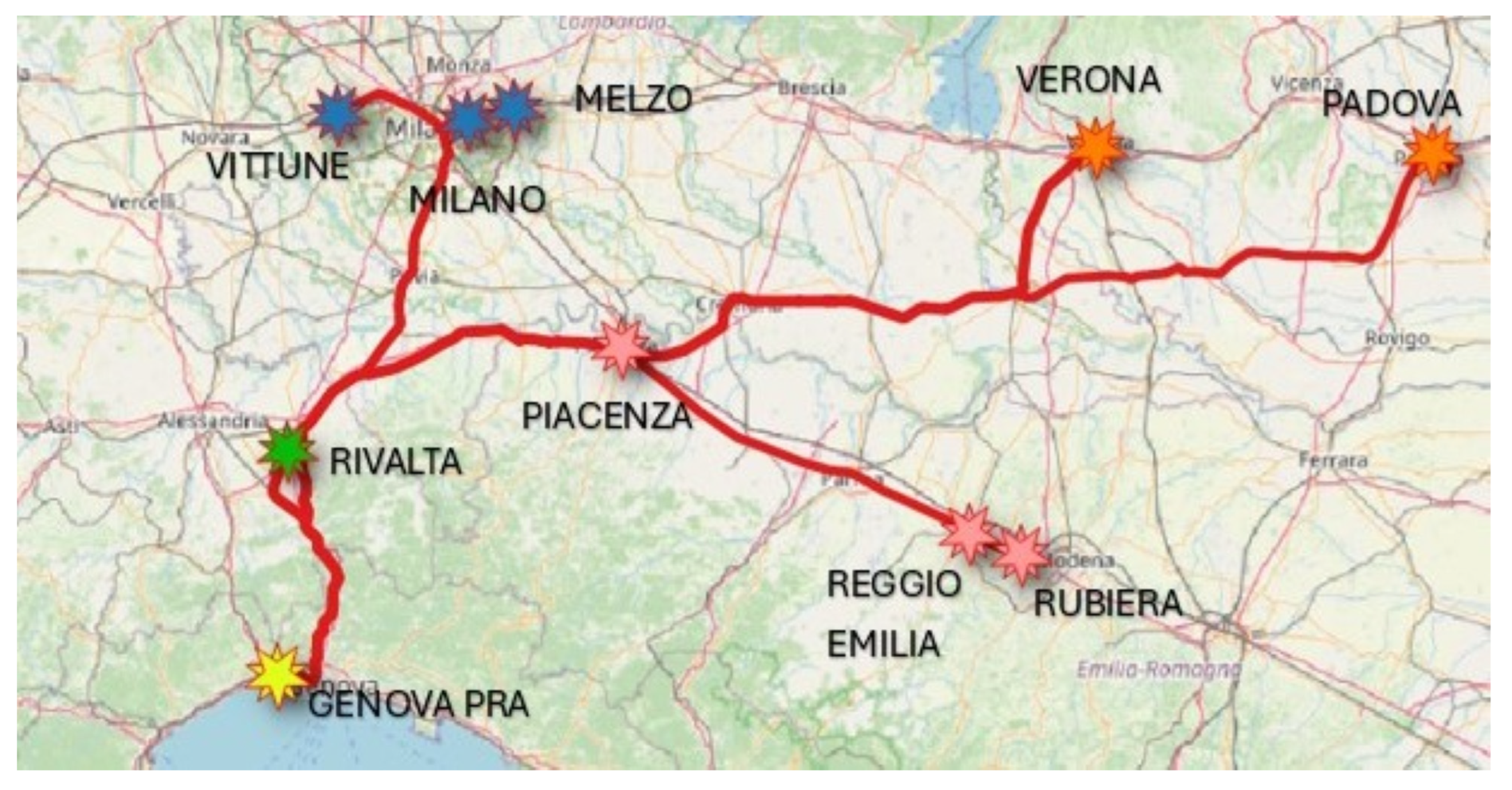
For the selection of the interports served by rail from the terminal we referred to [24], where the following destinations are listed: Milan (including Melzo and Vittuone), Rivalta (including Alessandria), Piacenza, Padua, Verona, and Reggio Emilia (including Rubiera). The map of the considered north-western Italian zone where terminal Pra is located is reported in Figure 1. Figure 1 also shows the railway network connecting the port terminal of Genoa PRA to the main interports it serves. The visualizations of the nodes of the network have been realized within this study using QGIS3.34.3 software [27] and OpenStreetMap [28].

The number of trains leaving the terminal for each destination was obtained from the data contained in the files generated by the ContainerFlow_Simulator program described in Bruzzone et al., 2024 [26], calculating the container percentages for each destination and assuming a time horizon of one semester. Then, we used these values to divide the trains among the four tracks, thus obtaining the values shown in

Table 2. distribution of departed trains to various destinations.

Destinations	# Containers	# Trains
Milano	24,853	22
Rivalta	5038	4
Piacenza	868	1
Padova	7714	7
Verona	19,113	17
Reggio Emilia	11,265	10

. These data allowed us to decide the container routing rules in the discrete-event simulation model presented in Section 4. Note that in total we had 68,851 containers and 60 departed trains.

3. Train Departure Planning

From the frequency and capacity of the railway line described in the previous section, the weekly train departure times were generated randomly using a procedure implemented in MATLAB. The values are generated according to the different policies allowed for the terminal’s rail container forwarding management, which will be evaluated later using the simulation model described in Section 4. To develop the departure schedules, the MATLAB procedure requires the following input data:

• total trains per week;
• destinations to be served;
• number of trains per week per destination;
• number of trains per day.

About the last two figures on the list, which have not yet been illustrated, different scenarios were used to choose the number of leaving trains per day. In particular, the following cases were considered to assess their impact on terminal performance in response to different scheduling:

• evenly distributed departures;
• departures distributed over medium-, low-, and high-frequency days;
• departures distributed over low- and high-frequency days only.

The procedure generates a schedule of train departures, specifying their track, departure time, and destination. Furthermore, we considered an added constraint to avoid, if possible, the departure of two consecutive trains to the same destination.

Currently, trains leave from the terminal tracks at the appointed time to connect to the national rail network. Therefore, no control is conducted on the number of containers loaded on the train (i.e., the percentage of the train load) and the number of containers waiting in the yard for the same destination. As far as the frequency of train departures is concerned, Scenario 1, described below, is followed.

Starting from the current operational rule of the train departures, the following two different management policies are proposed and compared to possibly improve the current performance indices.

Flexible Delay Policy: A delay in departure up to a maximum of 30 min is allowed, provided that the load level does not exceed 70% of the maximum capacity of the train. When the train is ready for departure, the load percentage is checked. If the load exceeds 70% of the maximum capacity, the train leaves at once. Otherwise, it is checked whether there are containers in the yard with the same destination as the train. If the number of such containers exceeds a predefined threshold (equal to 5), the train waits up to 30 min to allow for these containers to be loaded.

Strict Load Adherence Policy: If at the scheduled departure time the train does not reach 70% of its largest load, the next train is deleted, and the current train continues to be loaded. The departure of the train is then rescheduled to the time when the delayed train was originally supposed to leave.

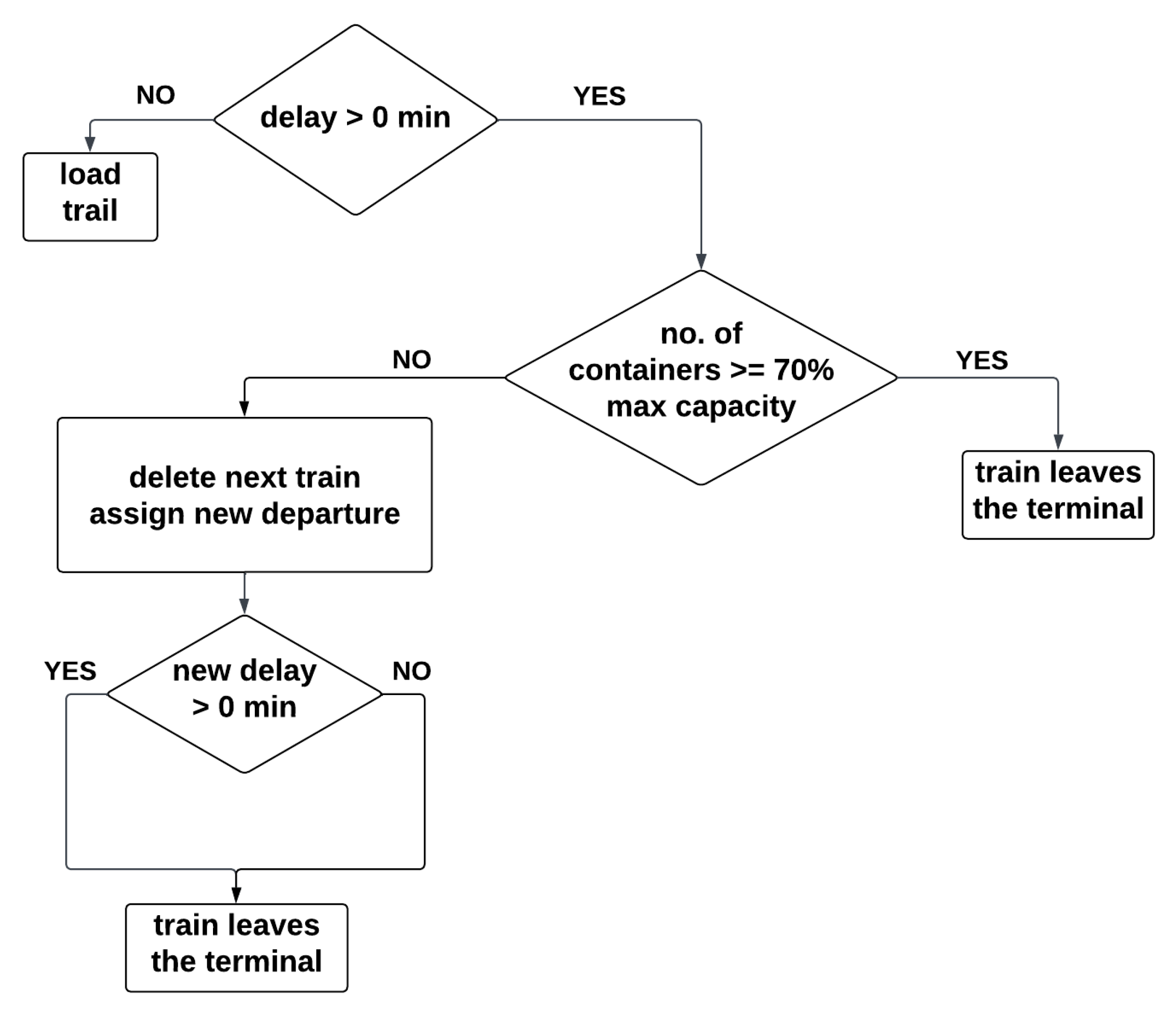
The diagram of the operations performed according to the Flexible Delay Policy is shown in Figure 2. In practice, when the departure time is reached, two checks are conducted:

• load percentage check: if the load is greater than 70%, the train leaves. Otherwise, the train loading process continues;
• container availability check for the train’s destination: if the number of containers available in the yard waiting for being loaded onto a train is less than a given value (i.e., 5), the train is not delayed and leaves. Otherwise, the loading process continues until the maximum delay of 30 min is reached.

Note that, as can be seen from the diagram reported in Figure 3, in the case of the Strict Load Adherence Policy, no delays are allowed, but if the train has not reached the required load levels, the train does not depart, causing it to be cancelled and the next train to wait. In practice, when the departure time is reached, the load percentage is checked. If this percentage does not reach 70% of the largest load, the scheduling of train departures is changed as follows: the train being loaded assumes a new departure time, corresponding to the time of the train leaving later. It is then necessary to update the departure time and remove the next one. This procedure can only be performed once, after which, once the new departure time has been reached, the train leaves regardless of the current load level.

As these data were not available, a procedure implemented in MATLAB was developed to obtain the weekly train departure times. The number of trains scheduled to leave from the terminal each day thus generated is shown in

Table 3. Number of daily leaving trains.

	Scenario 1	Scenario 2	Scenario 3	Scenario 4	Scenario 5
Sunday	0	0	0	0	0
Monday	3	3	10	15	20
Tuesday	11	11	10	5	0
Wednesday	16	16	10	15	20
Thursday	11	16	10	5	0
Friday	16	11	10	15	20
Saturday	3	3	10	5	0

. It should be noted that a total of 60 trains are scheduled to leave from the four available tracks each day.

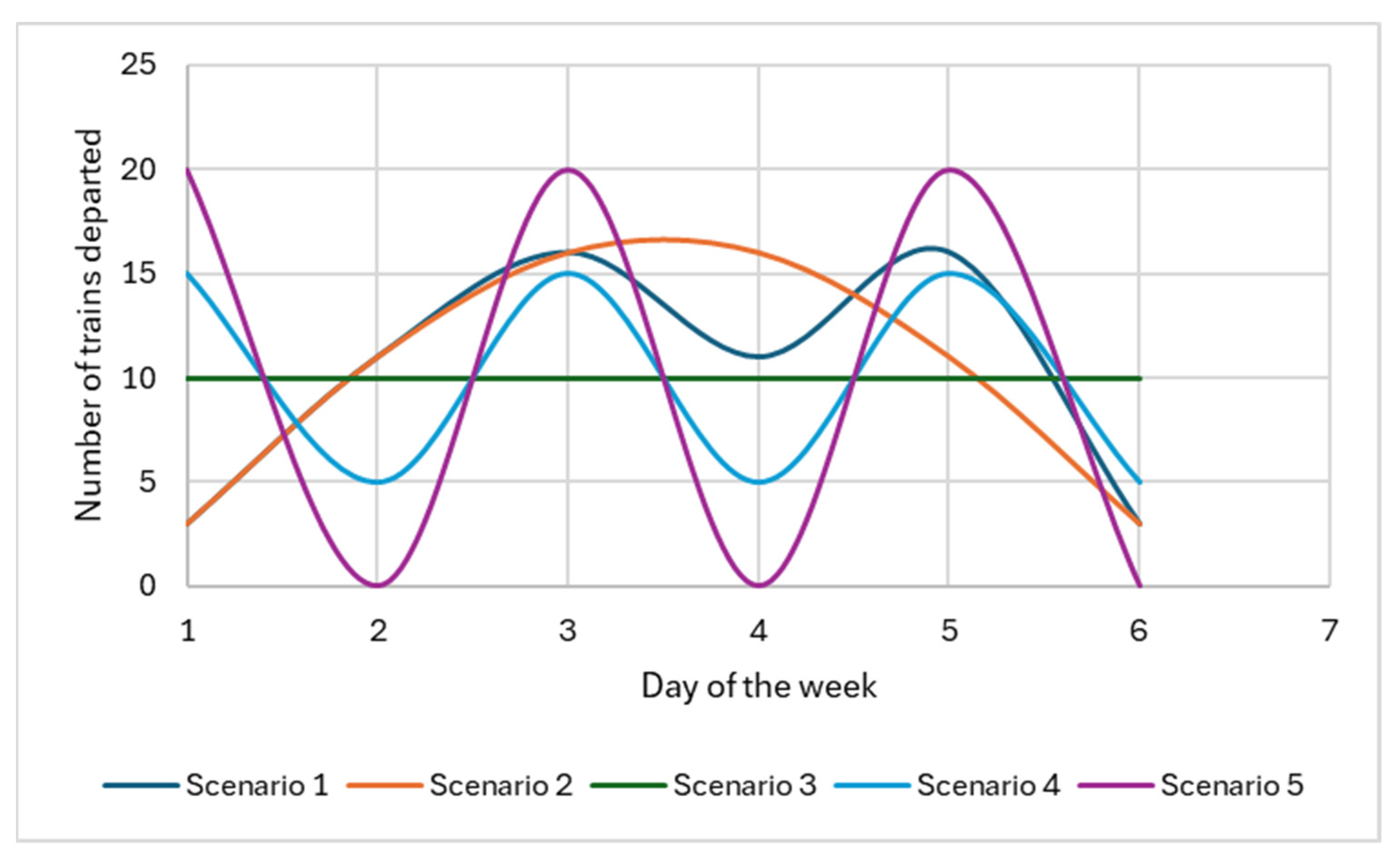
From the values given in Table 3, different scenarios for scheduling train departures were generated. It is worth noting that in setting up the scenarios illustrated in Figure 4, since the departure of trains involves their forwarding on the main rail network, the main constraint considered was to leave a fixed number of trains, i.e., 60, over the course of a week. Consequently, the frequency of daily departures was varied to assess its impact on the parameters under analysis. The derived scenarios are reported in Figure 4:

• Scenario 1: Trains are distributed according to their daily frequency. Trains are then classified into three types throughout the day according to their departure frequency, i.e., medium-, high-, and low-frequency;
• Scenario 2: The same distribution as described in Scenario 1 is used, but the high-frequency days are adjacent;
• Scenario 3: An even distribution of train departures over six days from Monday to Saturday is used. An equally distributed number of trains is then allocated to these days;
• Scenario 4: Low-frequency and high-frequency days are considered. The trains are then distributed over three low-frequency days and three high-frequency days;
• Scenario 5: A homogeneous distribution of train departures over the three middle days of the week is considered.

4. The Discrete-Event Simulation Model

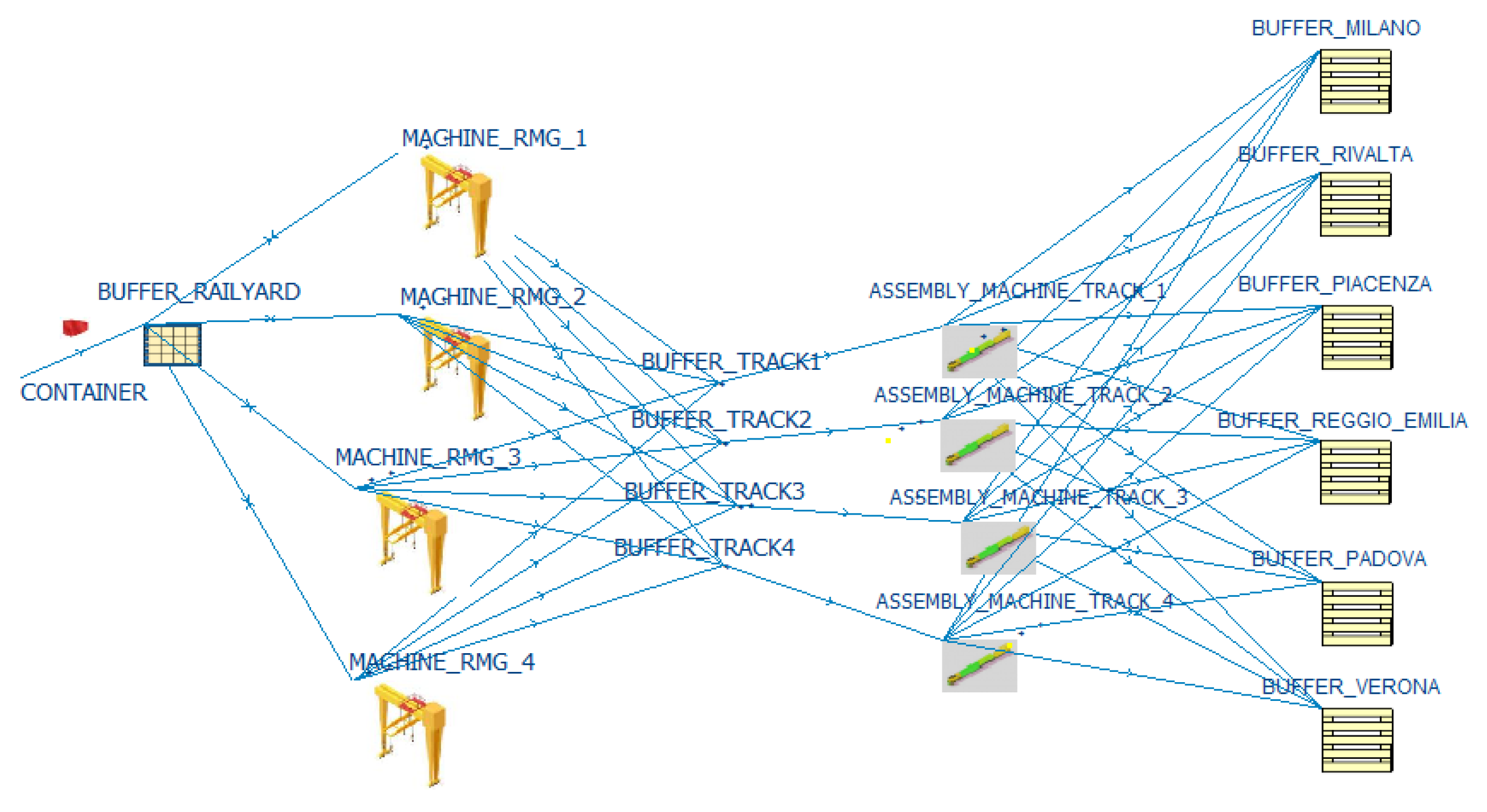
The discrete-event dynamic simulation study related to the problem at hand was implemented in Witness Horizon v.24, whose functionalities are described in Waller 2012 [29,30]. The layout of the reference terminal is shown in Figure 5. It is worth noting that we have only considered the layout related to the process of container handling, from their arrival at the terminal platform to their loading onto a train for their inland forwarding.

As can be seen from Figure 5, there are 11 buffers in the model, corresponding to waiting areas for the containers, and eight machines, corresponding to equipment of the terminal.

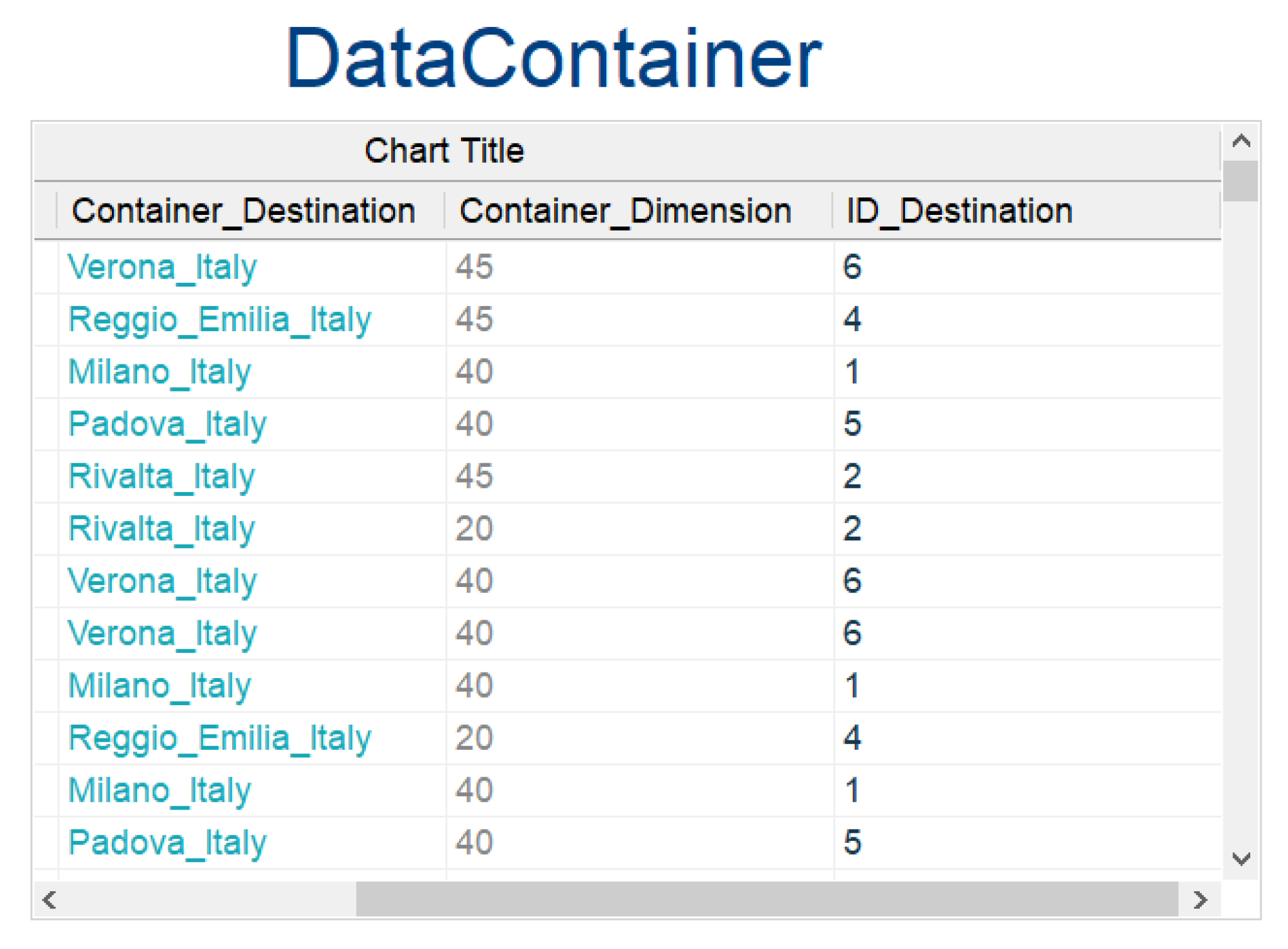
In the model, containers stand for the dynamic components, denoted parts. The containers are generated using a NegExp distribution with an average time of 5.7 min. This value is calculated based on the average number of annual import containers leaving by train from the terminal in Pra, as derived and reported in Table 1. The required information about the parts is obtained by reading the data table ‘DataContainer’ provided in the input file format .csv generated by using the ContainerFlow_Simulator described in Bruzzone et al., 2024 [26], as shown in Figure 6. Each column of the data table corresponds to an attribute of the container created, specifically: destination, expressed as a numerical value, and size (20′, 40′, or 45′).

Concerning the buffer, the railyard one is the container storage area close to the rail network. Within this simulation model element, the computation of the number of waiting containers for each destination is conducted by creating proper input and output actions. For this purpose, the variable disposition_i is defined, where i is the identification code of the corresponding destination. Then, the following action rules are considered within the dispatching rules to the railyard out from buffer:

$$action on input: if containe{r}_{destination}=i do dispositio{n}_i=dispositio{n}_i+1$$

$$action on output: if containe{r}_{destination}=i do dispositio{n}_i=dispositio{n}_i-1$$

As an output option from the buffer, a conditional rule is chosen requiring that the container destination attribute corresponds to one of the destinations associated with a train being loaded in one of the four tracks. The rule is as follows:

If container_destination = train_destination1 ∨ train_destination2 ∨ train_destination3 ∨ train_destination4

Furthermore, with reference to the model illustrated in Figure 5, the six buffer destinations represent the arrival interports. In each of them, the number of arriving trains is counted. This information allows us to compare the train management policies adopted.

Concerning the machines, we considered four rail-mounted gantry cranes (RMGs) used to move containers from the yard to the trains. We assumed an Erlang distribution as the handling cycle, whose average value is 5 min with the parameter K = 3. This distribution is considered to be the most appropriate because conditional cycles are used within the machinery exit rules, which will be described shortly. The RMG exit management rule checks two factors: the first is the destination of the container, comparing the destination attribute with the destinations of the trains to be loaded. Secondly, the available space onboard the train is controlled by the control_dimension function. This function returns a value between 0 and 3, depending on the space available onboard each train, according to the following operational condition:

$$control dimension=\left\{\begin{array}{c}0 \mathrm{can} \mathrm{load} \mathrm{any} container\\ 1 \mathrm{can} \mathrm{load} {20}^{\prime }e {40}^{\prime } container\\ 2\mathrm{can} \mathrm{load} {20}^{\prime } container\\ 3\mathrm{no} \mathrm{more}\mathrm{space}\end{array}\right.$$

The implemented control rules are then linked together so that containers are loaded onto the train with the correct destination and only if there is sufficient space. This control procedure is synthetized in Figure 7. It is worth noting that the order in which the trains are selected to execute the cycle described in Figure 7 affects the train loading percentage. In fact, if there were two trains with the same destination on two tracks and the control was always carried out in the same order, the first train would always be loaded, and the second would remain empty. To avoid this situation, each RMG crane used to load the trains has a different train control order.

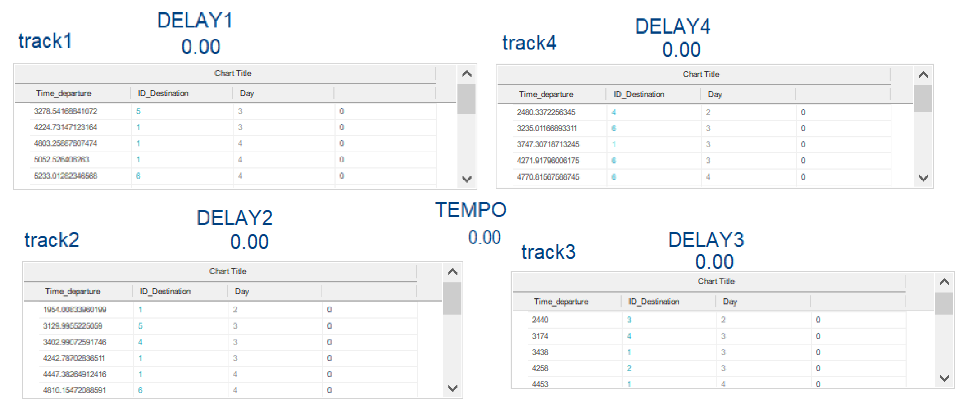
Finally, a buffer (Buffer_Track_N) and an assembly machine (assembly_track_N), both relating to the same track N, are used to represent the loading of trains and their departure. In particular, the buffer input action allows counting the containers that are loaded, considering their size, and thus the space (in percentage) occupied each time. The recognition of the departure time and destination to be assigned to the train is carried out by means of four data tables called Track_i. These data tables are an integral part of the simulation model and are depicted in Figure 8. The tables read as input the .csv files generated by MATLAB with the weekly scheduling. When each train leaves, the timetable cell, expressed in minutes, is updated with the following week’s timetable in this way:

train_departure = train_departure + 7 × 60 × 24

The assembly machine, on the other hand, assembles the departing containers by generating a train. The assembly action takes place according to the planned train departure strategies described above, namely the Flexible Delay Policy and Strict Load Adherence Policy.

To run the model and reproduce the operating scenario of the reference terminal, the following time shifts were implemented in the simulation models:

• shift 1: the terminal runs 24 h a day, every day of the year (except Christmas day and 1 May). Container arrivals follow this shift;
• shift 2: operators can work in the railway yard from 6 a.m. to 10 p.m. every day of the year (except Christmas day and 1 May). This shift is used for the RMGs in the yard;
• shift 3: trains can run from 6:00 a.m. on Monday to 6:00 a.m. on Sunday.

5. Simulation Results

The simulation experiment was conducted on a computer with the following technical specifications: 11th Gen Intel(R) Core (TM) i7-1165G7 @ 2.80GHz (2.80 GHz) x64-based processor, 16.0 GB (15.8 GB usable) installed RAM, and a 64-bit operating system. To verify the steady-state conditions (see, e.g., Law 2015 [31]), 33 independent runs were executed with different seeds, using a skip between seeds of value 100. Each simulation was conducted over a time horizon of 6 months. Moreover, an initial warmup period of 2 months was considered, corresponding to one-third of the total analysis period of this study. For each scenario under analysis, it was possible to run the instances automatically thanks to Witness Horizon’s experimenter option. This option allows the number of runs, seed skip value, warm-up time, and total simulation time to be set initially. The use of this resource simplified the process, allowing simulations to be run automatically. This approach ensured efficient management of time and computational resources.

The first step of our simulation experiment was to reproduce the actual behavior of the import containers from their arrival to their loading onto trains. Therefore, from the data shown in Table 1 and Table 2, we applied the train-departing rules currently used in the terminal described in Section 3, thus obtaining the main performance indices reported in

Table 4. Performance indices of the train loading operations in the present scenario.

Dwell Time	# Trains Departed	# Trains with Less than 70% of Max Load
6128	1549	1265

, that is, the number of departed trains and the number of departed trains having a load level less than 70%. The results reported in Table 4 show that 82% of trains leave with a load less than 70% of their maximum capacity.

The first test of the developed simulation model was dedicated to the evaluation of the goodness of the results and the accuracy of the model itself. This test was performed on the dwell time of the containers in the railyard considering the t_n−1-Student confidence interval, with a 95% degree of confidence, and by executing 33 independent runs, as shown in Figure 9.

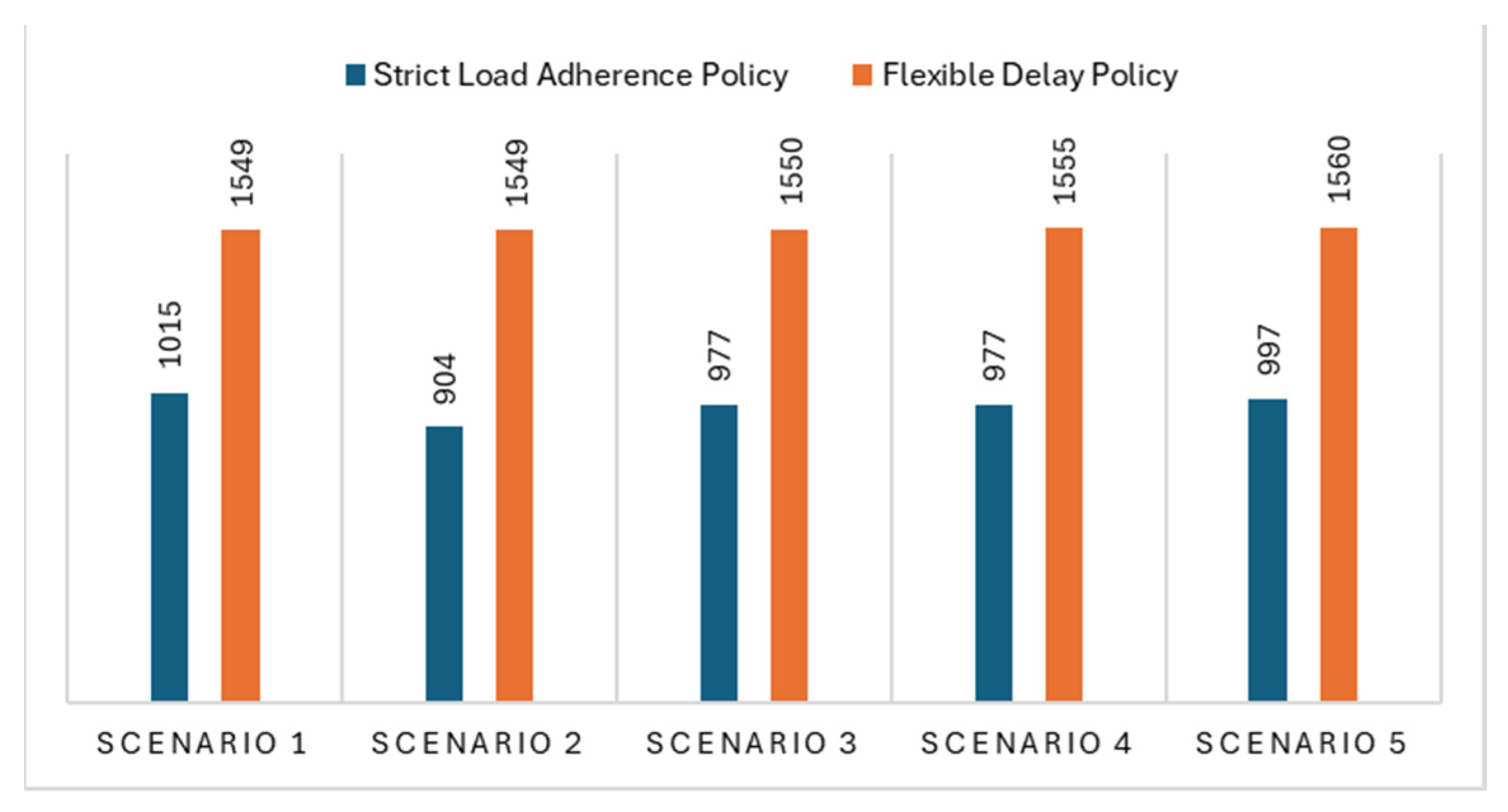
As a first analysis of the simulation experiments, we tested the impact of train departure policies on the waiting times of containers in the railyard buffer. The results show that the Strict Load Adherence Policy train departure rule results in an increase in the dwell time of containers in the buffer. This behavior is illustrated in Figure 10. The number of trains leaving from the terminal in the two departure management scenarios is reported and compared in Figure 11. As shown in Figure 11, by adopting the Strict Load Adherence Policy, the number of leaving trains, and thus the number of containers handled by the port, decreases. In practice, avoiding delays in train departures leads to a decrease in the overall efficiency of the transport system, increasing the average time that containers spend in the yard before being loaded onto trains.

Table 5. Increase in dwell time and decrease in train departure.

	Increase in Dwell Time	Decrease in Trains Departed
Scenario 1	10,188	534
Scenario 2	10,951	645
Scenario 3	13,204	573
Scenario 4	10,588	577
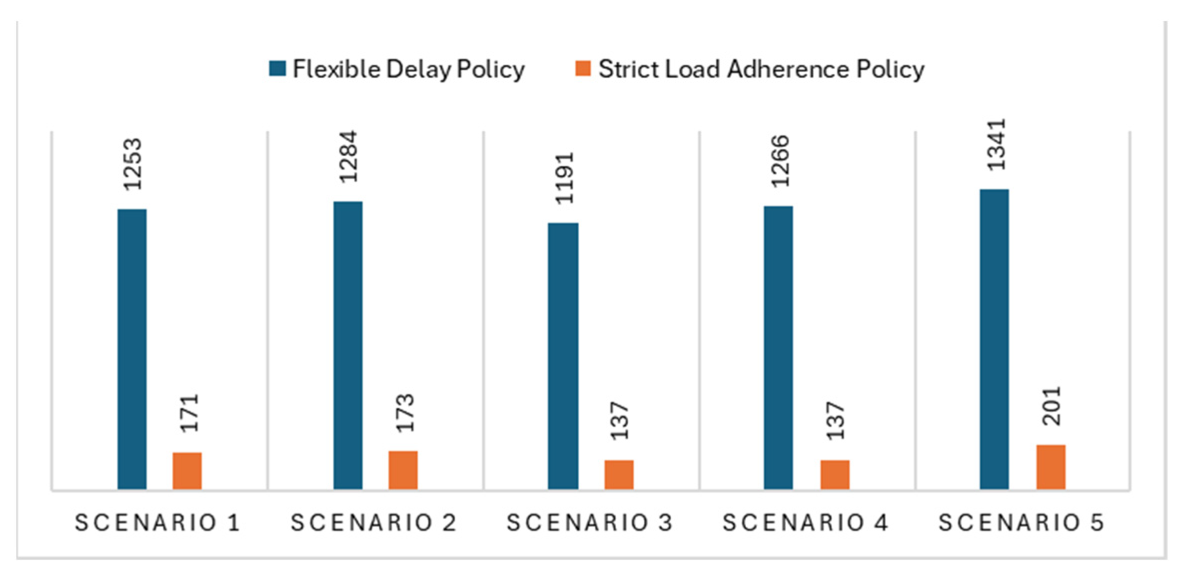
Scenario 5	6785	563

shows that the percentage increases in dwell times do not have a linear relationship with the reduction in the number of leaving trains. This nonlinear relationship between the two analyzed indices suggests that an increase in dwell time does not lead to a proportional decrease in the number of leaving trains. This implies that factors other than the number of leaving trains influence the dwell time of containers in the buffer. To make the most of this relationship, it is important to consider load and dwell time management policies based on specific aims. For example, the Flexible Delay Policy might be useful in scenarios where it is necessary to reduce dwell times and improve train load efficiency. Conversely, the Strict Load Adherence Policy might be preferable when the aim is to increase train load rates, even if this means longer dwell times. The use of simulation models to assess the impact of different policies can help make informed decisions and balance efficiency and load according to operational needs. The number of trains leaving with less than 70% of the largest load was also considered. The results of this analysis show that the Flexible Delay Policy increases the loading efficiency of trains, as the comparison in Figure 12 shows. The difference between the two train departure policies shows that, using the Flexible Delay Policy, the terminal experiences lower container dwell times. In contrast, the Strict Load Adherence Policy allows trains to increase their load percentage, improving the overall efficiency of the transport system. This shows that although the Flexible Delay Policy reduces the dwell time of containers, it results in lower loading efficiency of trains. In contrast, the Strict Load Adherence Policy ensures more loaded trains, albeit at the cost of longer container dwell time in the buffer.

From the analysis of the scheduling scenarios for the Flexible Delay Policy, reported in

Table 6. Flexible Delay Policy results.

Scenario	Dwell Time	# Trains Left	# Trains with Less than 70% of Max Load
Scenario 1	5292	1549	1253
Scenario 2	7159	1549	1284
Scenario 3	3271	1550	1191
Scenario 4	4819	1555	1266
Scenario 5	8409	1560	1341

, it is evident that Scenario 3, with homogeneous departures for each day, is the best in terms of average delays, dwell times, and number of leaving trains with a load of less than 70 percent. In fact, this scenario reduces all these parameters, proving greater overall operational efficiency. It is interesting to note, however, that Scenario 1, which is closest to the scheduling policy currently adopted by the terminal under analysis, does not appear to be the best in any of the parameters considered. This scenario excels neither in reducing average delays nor in minimizing dwell times and the number of leaving trains with suboptimal loads. The results reported in Table 6 show that the percentage of trains leaving with a load less than 70% of maximum capacity is between 77% and 86%.

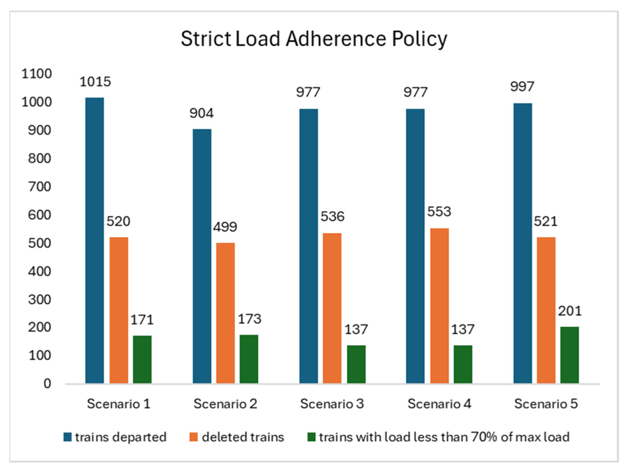
From the analysis of the load adherence policy, shown in Figure 13 and

Table 7. Strict Load Adherence Policy results.

Scenario	Dwell Time
Scenario 1	15,480
Scenario 2	18,110
Scenario 3	16,475
Scenario 4	15,407
Scenario 5	15,194

, it is interesting to note that each scheduling scenario improves only one parameter at a time, with no obvious simultaneous improvements on multiple parameters. The results reported in Figure 13 show that the percentage of trains leaving with a load lower than 70% of maximum capacity is between 14% and 20%. One noteworthy finding is the significant reduction in the number of trains leaving with less than 70 percent load in Scenarios 3 and 4. However, both policies keep a comparable number of trains leaving with a load below 70%. Moreover, both policies keep a comparable number of cancelled trains as in the other scenarios. Scenario 2, on the other hand, has the highest dwell time among the five scenarios analyzed. This suggests that although some policies may improve specific operational aspects, such as train load percentage, other areas may be negatively affected, as shown by the increase in dwell time in Scenario 2.

These observations highlight the complexity of improved terminal management and the importance of balancing various operational parameters to achieve overall efficiency. Future research should aim to develop scheduling strategies that can improve multiple parameters simultaneously, reducing train cancellations and optimizing dwell times and capacity.

6. Conclusions

In this paper, we dealt with train loading procedures in a container terminal. In particular, starting from the current level of operations, we examined whether it is possible to improve the performance indices of interest, making the most of the digitization and visualization procedures of the data currently present in the terminal. The indices we examined were the dwell time, the average number of containers loaded on a train, and the load level of trains waiting at the yard.

The proposed policies do not require additional resources but merely variations, obviously permissible, of the current operating rules. To test the validity of the proposed policies, which also include possible variations in train departure frequencies on a weekly basis, a discrete-event simulation model was implemented with Witness. The results obtained by running several independent simulations with different scenarios are very promising. We have demonstrated that it is possible to improve the above-mentioned performance indices by making minimal changes, provided that the necessary information, i.e., the destination of the trains, the number of containers to be loaded and already loaded, is available on digital platforms, such as those used within the Witness simulation software environment. Among the most significant results are that the Flexible Delay Policy allows a reduction in dwell time in the range from 5 to 48 h, while the Strict Load Adherence Policy reduces the percentage of the number of departing trains with a load less than 70% from 82% to 17%. It should be emphasized that the proposed operational rules are easy to implement, and therefore, by having a data digitization system with the necessary information, it is possible to truly adapt them to the actual needs of the terminal and increase its operational efficiency. As a future development of this research, we intend to extend this case study, where only standard containers are considered, to the case where there are also refrigerated containers and containers with dangerous goods. These containers obviously have different rules and priorities in the management of loading operations and constraints on waiting time. Moreover, we wish to analyze how external factors, such as weather or geopolitical events and environmental issues, influence the train departure strategies discussed in this study.