Article

Advanced Queueing and Location-Allocation Strategies for Sustainable Food Supply Chain

by
Amirmohammad Paksaz
1,
Hanieh Zareian Beinabadi
2,
Babak Moradi
3,
Mobina Mousapour Mamoudan
4 and
Amir Aghsami
5,*
1
School of Industrial Engineering, Iran University of Science and Technology, Tehran 16846-13114, Iran
2
Industrial Engineering Department, Islamic Azad University, North Tehran Branch, Tehran 16511-53311, Iran
3
Department of Industrial Engineering, Faculty of Mechanical Engineering, University of Tabriz, Tabriz 51656-87386, Iran
4
School of Industrial Engineering, College of Engineering, University of Tehran, Iran 14155-6619, Iran
5
Department of Industrial Engineering, Ankara Yıldırım Beyazıt University, Ankara 06010, Turkey
*
Author to whom correspondence should be addressed.
Logistics 2024, 8(3), 91; https://doi.org/10.3390/logistics8030091
Submission received: 4 July 2024 / Revised: 7 September 2024 / Accepted: 9 September 2024 / Published: 14 September 2024
(This article belongs to the Section Sustainable Supply Chains and Logistics)

Abstract

:
Background: This study presents an integrated multi-product, multi-period queuing location-allocation model for a sustainable, three-level food supply chain involving farmlands, facilities, and markets. The model employs M/M/C/K queuing systems to optimize the transportation of goods, enhancing efficiency and sustainability. A mixed-integer nonlinear programming (MINLP) approach is used to identify optimal facility locations while maximizing profitability, minimizing driver waiting times, and reducing environmental impact. Methods: The grasshopper optimization algorithm (GOA), a meta-heuristic algorithm inspired by the behavior of grasshopper swarms, is utilized to solve the model on a large scale. Numerical experiments demonstrate the effectiveness of the proposed model, particularly in solving large-scale problems where traditional methods like GAMS fall short. Results: The results indicate that the proposed model, utilizing the grasshopper optimization algorithm (GOA), effectively addresses complex and large-scale food supply chain problems. Compared to GAMS, GOA achieved similar outcomes with minimal differences in key metrics such as profitability (with a gap ranging from 0.097% to 1.11%), environmental impact (0.172% to 1.83%), and waiting time (less than 0.027%). In large-scale scenarios, GOA significantly reduced processing times, ranging from 20.45 to 64.78 s. The optimization of processing facility locations within the supply chain, based on this model, led to improved balance between cost (up to $74.2 million), environmental impact (122,112 hazardous units), and waiting time (down to 11.75 h). Sensitivity analysis further demonstrated that increases in truck arrival rates and product value had a significant impact on improving supply chain performance.

1. Introduction

The global demand for food is projected to quadruple over the next decade. According to Muchhadiya et al. [1], the current global population of approximately 7.8 billion is expected to reach 9.7 billion by 2050, leading to a substantial increase in food demand. This surge underscores the critical importance of effective food supply chain (FSC) management. Due to the perishable nature of food products, managing FSCs is inherently more complex than other supply chains. Moreover, the environmental impact of human activities has drawn significant attention, particularly the need to mitigate adverse effects. One critical factor contributing to environmental impact is the transportation fleets that move products through the supply chain, especially those waiting in loading queues. Consequently, FSC leaders face numerous challenges in enhancing system efficiency and effectiveness while maintaining product quality and controlling supply chain costs. Optimal decisions regarding the location of processing facilities and warehouses are pivotal as they directly influence product quality, demand coverage, and overall supply chain profitability.
This study advances the existing literature by incorporating M/M/C/K queuing systems for farmland and processing facilities, an area previously unexplored. The primary aim is to reduce vehicle waiting times, which directly impact driver utility and overall supply chain profit. Additionally, this research addresses the location-allocation problem for processing facilities and markets, optimizing facility locations and market allocations while considering CO2 emissions from transportation vehicles. This dual consideration of environmental impact and operational efficiency is often overlooked in existing research.
The research aims to address the following key research questions:
  • What are the optimal locations for processing facilities to ensure efficient operation of the supply chain?
  • How can the food supply chain be designed to minimize environmental impact, particularly in terms of vehicle emissions?
  • What are the factors affecting vehicle waiting times at farms and processing facilities, and how can these times be optimized?
Our study introduces an integrated multi-product, multi-period queuing location-allocation model within a green, three-level food supply chain comprising farmlands, facilities, and markets. The proposed model employs M/M/C/K queuing systems for vehicles transporting crops from farmlands to processing facilities and delivering products to markets. It aims to identify optimal facility locations, reduce vehicle queue times (impacting both driver utility and environmental impact), and maximize supply chain profit while minimizing driver waiting time and environmental impact. The model is solved exactly for small problems, and a metaheuristic algorithm, the grasshopper optimization algorithm (GOA), is developed for large-scale problems due to their complexity and computational demands. The model’s applicability is demonstrated through a case study in the rice industry of Babol, Iran. The primary contribution of this paper is the simultaneous consideration of location-allocation and two M/M/C/K queuing systems for vehicles in both farmlands and processing facilities within a food supply chain, including environmental impact considerations.
The paper is structured as follows: Section 2 presents the literature review. Section 3 outlines the problem definition and mathematical formulation. Section 4 details the model validation and algorithm performance. Section 5 covers the case study and data analysis. Section 6 discusses real-case applications. Section 7 concludes with the findings and future research directions.

2. Literature Review

This section provides a concise review of various research approaches, including sustainability and queuing systems within the supply chain.

2.1. Approaches in Supply Chain Management

Supply chain management (SCM) has evolved significantly over the years, incorporating various approaches to address the complexities and challenges inherent in global supply networks. One critical approach is sustainability, which has become increasingly important due to rising environmental awareness and regulatory pressures. Research in this area emphasizes the need for green supply chains that minimize environmental impact while maintaining economic viability. Studies by Srivastava [2] and Sarkis [3] highlight the adoption of green practices such as recycling, waste reduction, and the use of renewable energy in supply chains. Furthermore, Carter and Rogers [4] discuss sustainable procurement strategies that integrate environmental considerations into sourcing decisions, emphasizing supplier collaboration and long-term partnerships. Life Cycle Assessment (LCA), advocated by researchers such as Guinée et al [5], evaluates the environmental impact of products throughout their lifecycle, from raw material extraction to disposal.
Another significant approach in SCM is the application of queuing theory to various aspects of supply chain management to optimize operations and reduce delays. Zipkin [6] explored the application of queuing models to inventory systems, demonstrating how these models can predict stock levels and reorder points to minimize waiting times and stockouts. In transportation logistics, research by Daganzo [7] focused on the use of queuing theory to improve scheduling and routing, reducing vehicle idle times and enhancing delivery efficiency. Additionally, studies like those by Gross [8] examine queuing systems in service facilities within supply chains, such as distribution centers and warehouses, to optimize service rates and reduce congestion, thereby enhancing the overall efficiency and responsiveness of supply chain logistics.
Integrating various aspects of supply chain management into cohesive models has also been a significant focus of recent research. David, Philip and Edith [9] discuss the development of integrated models that consider multiple levels of the supply chain, from suppliers to end customers, to optimize overall performance. The use of mixed-integer non-linear programming (MINLP) models to address complex decision-making problems in SCM, including facility location and inventory control, is highlighted by Perea-Lopez, Ydstie and Grossmann [10].

2.2. Queueing Approach in Supply Chain Management

Queuing theory has been extensively applied in supply chain management to optimize various processes and reduce inefficiencies. This literature review explores key research contributions that utilize queuing approaches to enhance supply chain performance, focusing on inventory management, transportation logistics, service facilities, and integrated models.
Queuing models are widely used to manage inventory systems by predicting stock levels and reorder points, thereby minimizing waiting times and stockouts. Zipkin [6] explored the application of queuing models to inventory management, demonstrating their effectiveness in maintaining optimal stock levels. Similarly, Gross [8] discusses the fundamentals of queuing theory and its application in various supply chain contexts, highlighting its role in reducing congestion and improving service rates. Recent advancements include the work of Kolahi-Randji, Attari and Ala [11], who used discrete event simulation to enhance operational efficiency in a multi-level, multi-commodity detergent supply chain, demonstrating significant improvements in inventory cost management and overall system performance.
Transportation logistics within supply chains also benefit from queuing theory, particularly in optimizing operations and reducing delays. Buzacott and Shanthikumar [12] examined the application of queuing models in manufacturing and service systems, providing insight into how these models can improve throughput and reduce cycle times. Rabe [13] discusses the practical application of queuing theory in production systems, emphasizing its role in managing variability and improving workflow. Additionally, the study by Franceschetto and Amico [14] on supply chains in the automotive industry illustrates the benefits of a mixed centralized-decentralized approach for critical and non-critical product planning, showcasing improvements in system efficiency and responsiveness.
Integrated models that combine queuing theory with other optimization techniques have been developed to address complex supply chain problems. Perea-Lopez, Ydstie and Grossmann [10] highlight the use of mixed-integer non-linear programming (MINLP) models combined with queuing systems to optimize facility location and inventory control. In 2024, Amellal and Amellal [15] introduced an advanced integrated model utilizing machine learning for sentiment analysis, demand forecasting, and price prediction, significantly improving strategic decision making and resource allocation.
Recent studies have also focused on the environmental impact of supply chain activities, incorporating queuing models to minimize adverse effects. Srivastava [2] highlights the importance of incorporating environmental considerations into supply chain management, advocating for the use of queuing models to achieve greener operations. Mohtashami, Aghsami and Jolai [16] present a green, closed-loop supply chain design using queuing systems to reduce environmental impact and energy consumption. This study emphasizes the importance of integrating environmental concerns into supply chain models to enhance sustainability. Masoumi and Aghsami [17] integrated an M/M/C/K queuing system into an inventory routing problem to address congestion and response times for post-disaster humanitarian relief. The case study focuses on optimizing the delivery of relief supplies by considering the complexities of congestion and operational delays. The model aims to improve the efficiency and responsiveness of humanitarian logistics, ensuring timely delivery of aid to affected areas. Aghsami and Abazari [18] present a comprehensive approach to optimizing blood supply chain management. The study addresses critical issues in blood supply chains, such as cost efficiency and donor satisfaction, by incorporating a finite capacity queuing system into the supply chain model. Karamipour and Kermani [19] present a mathematical model to optimize blood supply chains by improving the efficiency of collection centers using an M/M/C/K queuing system and developing a metaheuristic algorithm. This approach reduces wait times and operational costs, enhancing donor satisfaction and overall supply chain efficiency.
Further extending the application of queuing theory, Abbaspour et al. [20] explored an integrated queueing-inventory-routing problem in a green, dual-channel supply chain, considering pricing and delivery period in the context of a construction material supplier. This study demonstrates the importance of integrating multiple aspects of supply chain management to achieve optimal performance. Aghsami, Samimi and Aghaei [21] propose an integrated Markovian queueing-inventory model in a single retailer–single supplier problem with imperfect quality and destructive testing acceptance sampling. This model addresses quality control issues within supply chains, providing a robust framework for managing imperfect products.
In the realm of energy optimization, Deghoum et al. [22] highlight the importance of aerodynamic, steady-state, and dynamic analyses in the optimization of small horizontal axis wind turbines. This approach to optimization, while focused on energy efficiency, aligns with the principles of queuing theory in optimizing resource allocation and system performance, demonstrating the interdisciplinary applicability of optimization techniques across different fields.

2.3. Research Gaps and Our Contribitions

Upon reviewing the recent literature, it is evident that there are significant research gaps in the study of food supply chains, particularly in the incorporation of queuing systems. While most studies apply queuing systems to isolated parts of the supply chain, our research uniquely integrates M/M/C/K queuing systems across both farmlands and processing facilities. This integration adds complexity and realism to the modeling of food supply chains, especially when considering multiple crops and intermediate products within seasonal time windows.
Furthermore, unlike previous studies, this research simultaneously addresses the location-allocation problem for processing facilities while integrating queuing systems for both farmlands and facilities, with a specific focus on reducing the environmental impact of transportation. To the best of our knowledge, no prior research has comprehensively combined these aspects. Therefore, our study makes the following contributions:
  • Comprehensive Integration of Queuing Systems: Incorporating M/M/C/K queuing systems for vehicles in both farmlands and processing facilities, addressing a gap in holistic supply chain modeling.
  • Optimization of Facility Location and Allocation: Evaluating multiple potential sites and selecting optimal locations to efficiently allocate market demand.
  • Environmental and Operational Efficiency: Aiming to minimize CO2 emissions from trucks while maximizing total supply chain profit and reducing drivers’ waiting times by optimizing the number of active servers in both farmlands and facilities.
By addressing these gaps, our study provides a more realistic and comprehensive model of food supply chains, contributing to both the academic literature and practical applications in supply chain management.

3. Methodology

In this section, the problem definition and mathematical formulation are presented.

3.1. Problem Definition

The food supply chain (FSC) faces unique challenges due to the perishable nature of food products, which necessitates timely and efficient management of the entire supply chain to maintain product quality and minimize waste. Traditional supply chain models often fail to adequately address the complexities associated with the perishable nature of food products, as well as the environmental impact of transportation and logistics.
In recent years, queuing theory has been applied to various aspects of supply chain management to optimize operations and reduce inefficiencies. However, most studies have focused on the application of queuing systems to only one part of the supply chain, such as inventory management, transportation logistics, or service facilities. This fragmented approach overlooks the interdependencies between different stages of the supply chain, which can lead to suboptimal decision making and increased operational costs.
Moreover, the environmental impact of supply chain operations has become a critical concern, especially regarding the CO2 emissions generated by transportation fleets. There is a pressing need to develop models that not only optimize operational efficiency but also minimize environmental impact.
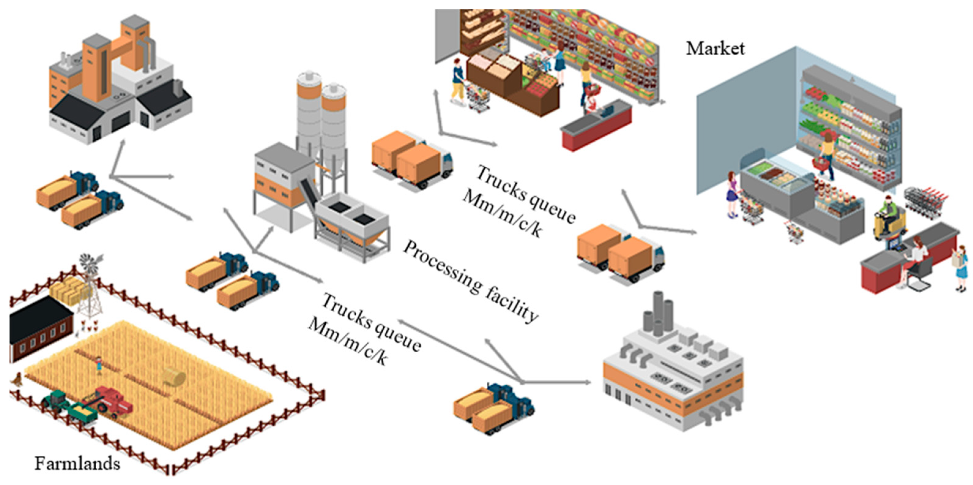
The current study presents a multi-product and multi-period queuing location-allocation problem in a three-level supply chain considering vehicles’ environmental impact. As depicted in Figure 1, vehicles load different crops in farmlands. An M/M/C/K queuing system is considered in farmlands to reduce the vehicle waiting time. After loading at the farm, the trucks allocate to the processing facilities. Each truck can ship crops to one or more processing facilities. There are a finite number of servers in facilities that unload the crops and start converting them to products. An M/M/C/K queuing system is considered at this level to reduce the trucks’ waiting time. In this stage, a location-allocation problem is considered to locate the facilities and allocate deterministic market demand. If needed, intermediate products move between facilities. Finally, vehicles load the products from the facilities and deliver them to each market. One of the critical objectives of the current study is to reduce the CO2 emissions produced by trucks in different stages during their waiting in lines and shipping. The developed model tries to maximize the supply chain’s total profit, minimize truck waiting time, and minimize the vehicles’ environmental impact.
The primary objective of this research is to address these gaps by developing an integrated multi-product, multi-period queuing location-allocation model for a green, three-level food supply chain, encompassing farmlands, processing facilities, and markets. The specific goals of this study are:
  • To incorporate M/M/C/K queuing systems for vehicles in farmlands and processing facilities, thus capturing the complexities and interdependencies between these stages.
  • To consider multiple crops and intermediate products, reflecting the diverse nature of agricultural production and processing.
  • To integrate the location-allocation problem for processing facilities with queuing systems, optimizing facility placement and market allocation.
  • To account for seasonal time windows and their impact on the supply chain, providing a realistic representation of agricultural operations.
  • To minimize the CO2 emissions from transportation activities, thereby addressing the environmental impact of the supply chain.
  • To maximize the total profit of the supply chain by reducing waiting times, optimizing facility locations, and improving overall operational efficiency.

3.2. Notations

Table 1, Table 2, and Table 3 respectively present the Index, Parameters, and Variables used in the study.

3.3. Mathematical Formulation

We proposed the following mathematical model for our problem.
M a x   Z 1 : L M T P S V A L p s Z l m t p s L T f c l t Y l t F L T C S O C T X f l t c s F L T C S P d r f l t c c X f l t c s L L T T I S d l l l o c t s i Q l l t t i s L L T T I S d l l l t c i Q l l t t i s L M T P S d m l m t c p Z l m t p s F μ f s F μ l t s
M i n   Z 2 : L L T T I S N d l l l × e t l l n × Q l l t t i s P C + 1 + L M T P S N d m l m × e t l m n × Z l m t p s P C + 1 + F L T C S N d r f l × e t f l n × X f l t c s P C + 1
M i n   Z 3 F S W f s + L T S W l t s
The objective functions (1)–(3) maximize the total profitability of the supply chain, minimize the total CO2 and other harmful gases, and minimize truck waiting time in the farm regions, respectively.
S.t:
L T X f l t c s   s u p f c s             f   ,   c   ,   s    
F C X f l t c s + L T I Q l l t t i s 1     c a p s   Y l t                   l , t , s
T Y l t   1             l    
L T Z l m t p s   d e m m p s             m , p , s
m Z l m t p s + L T Q l l t t p s = L T A I c f t p a c r t i a   Q l l t t i s 1     + L T Q l l t t p s 1 +   F C A c f t p a c r t c a X f l t c             l , t , p , s
p r e m p s         L T Z l m t p s             m , p , s    
Constraint (4) indicates that the quantity of crops c transported from farmland f is confined to the supply of farmland f. Constraint (5) ensures that product flow to a facility at location l of type t is only allowed when it is open. Constraint (6) depicts that only one facility can be open at location l. Constraint (7) creates an upper boundary on demand for product p at market m in season s. Constraint (8) shows the conversion of crops and intermediates to products. It shows a predicted readiness for each market by constraint (9).
π 0 f s = n = 0 c c f s 1 λ f s μ f s n n ! + λ f s μ f s c c f s c c f s ! k f s c c f s + 1 1           i f ρ F = 1
π 0 f s = n = 0 c c f s 1 λ f s μ f s n n ! + λ f s μ f s c c f s c c f s ! ( 1 ρ f s k f s c c f s + 1 1 ρ f s ) 1           i f ρ F 1
π k f f s = ( 1 c c f s k f s c c f s ) λ f s μ f s k f s c c f s ! ( π 0 f s )           f , s
Constraints (10) and (11) show the percent of servers’ idle time in farmland f. Constraint (12) depicts the percent of time unit when k trucks exist in the truck queue of farmland f.
L Q f s = λ f s μ f s c c f s π 0 f s c c f s ! ρ f s 1 ρ f s 2 1 ( ρ f s ) k f s c c f s + 1 1 ρ f s k f s c c f s + 1 ( ρ f s ) k f s c c f s           f , s
L f s = L Q f s + c c f s π 0 f s ( n = 0 c c f s 1 c c f s n λ f s μ f s n n ! )           f , s
W Q f s = L Q f s λ f s ( 1 π k f f s )     f , s    
W f s = L f s λ f s ( 1 π k f f s )           f , s  
ρ f s = λ f s c c f s μ f s           f , s
λ f s   ¯ = λ f s ( 1 π k f f s )           f , s
Constraint (13) determines the average queue length of each server in farmland f. Constraint (14) indicates the average length of staying in farmland f. Constraint (15) states the average waiting time in the queue of truck n in farmland f. Constraint (16) displays the average waiting time of trucks in farmland f. Constraint (17) applies the percent of servers’ working time in farmland f. The arrival rate of trucks to farmland f is specified by constraint (18).
L T X f l t c s λ f s   ¯ × p c             f , s
π 0 l t s = n = 0 c l l t s 1 λ l t s μ l t s n n   ! + λ l t s μ l t s c l l t s c l l t s ! k l t s c l l t s + 1 1   i f   ρ L = 1       l , t , s
π 0 l t s = n = 0 c l l t s 1 λ l t s μ l t s n   n   ! + λ l t s μ l t s c l l t s c l l t s ! ( 1 ρ l t s k l t s c l l t s + 1 1 ρ l t s ) 1   i f   ρ l 1               l , t , s
Constraint (19) allocates farm f to at least one of the processing facilities and ensures that processing facilities at location l will be loaded by at least one farm from region f. Constraints (20) and (21) display the percent of servers’ idle time in the processing facility at location l.
π k l l t s = ( 1 c l l t s k l t s c l l t s ) λ l t s μ l t s k l t s c l l t s ! ( π 0 l t s )             l , t , s
L Q l t s = λ l t s μ l t s c l l t s π 0 l t s c l l t s ! ρ l t s 1 ρ l t s 2 1 ( ρ l t s ) k l t s c l l t s + 1 1 ρ l t s k l t s c l l t s + 1 ( ρ l t s ) k l t s c l l t s             l , t , s
L l t s = L Q l t s + c l l t s π 0 l t s n = 0 c l l t s 1 c l l t s n   λ l t s μ l t s n   n   !             l , t , s
W Q l t s = L Q l t s λ f t s ( 1 π k l f t s )             l , t , s
Constraint (22) shows the percent of time unit when k trucks exist in the truck queue of a processing facility at location l. Constraint (23) determines each server’s average queue length in the processing facility at location l. Constraint (24) indicates the average length of staying in the processing facility at location l. Constraint (25) states the average waiting time in the queue of truck n in the processing facility at location l.
W l t s = L l t s λ l t s ( 1 π k l l t s )             l , t , s
ρ l t s = λ l t s c l l t s   μ l t s             l , t , s
λ l t s   ¯ = λ l t s ( 1 π k l l t s )             l , t , s
Constraint (26) displays the average waiting time of trucks in the processing facility at location l. Constraint (27) applies the percent of servers’ working time processing facility at location l. The arrival rate of trucks to the processing facility at location l is specified by constraint (28).
μ f s   U B L P             f , s
μ l t s   U B L P             l , t , s
μ f s   L B L P             f , s
μ l t s   L B L P             l , t , s
Constraints (29)–(32) create upper and lower boundaries for the rate of service in farmland f and processing facility at location l.
Constraints (33) and (34) state the operation and inaction cost functions of servers in farmland f and processing facility l.
F μ f s = A f μ f s + B f             f , s
F μ l t s = A l μ l t s + B l             l , t , s
L T I Q l l t t i s     L T Y l t × M                   l , t , s
L T p Q l l t t p s     L T Y l t × M       l , t , s
L T I Q l l t t i s     Y l t × M                   l , t , s
L T Z l m t p s   L T Y l t × M             m , p , s    
m Z l m t p s λ l t s   ¯ × p c             l , t , p , s    
y l t   0,1             f ,   l , t , s
x f l t c s   ,   q l l t t p s   ,   z l m t p s   ,   w   ,   w q   ,   λ   ¯ , π 0 ,   π k   0             f ,   l , t , c , p , k , s
Constraints (35)–(39) ensure the model’s validity. Finally, constraint (40) defines the type of variables used.

4. Solution Approach

The problem is solved on small and medium scales with an exact method in GAMS software. As solving the problem on a large scale with GAMS is not achievable in a reasonable time, we developed a metaheuristic algorithm (GOA). Moreover, in order to solve the multi-objective model, we applied the LP-metrics method.

4.1. Multi-Objective Solution Procedure

The LP-metrics method used in the current study is the appropriate choice to solve multi-objective models. Because this method can find the optimal answer with the shortest distance from the ideal solutions, it does so with less time and effort [23]. Equations (42)–(44) are used to implement the LP-metric method in a multi-objective model [24]:
M i n   L P   O B J = [ w e i g h t 1 × O b j e c t i v e 1 * O b j e c t i v e 1 O b j e c t i v e 1 * + w e i g h t 2 × O b j e c t i v e 2 O b j e c t i v e 2 * O b j e c t i v e 2 * + w e i g h t 3 × O b j e c t i v e 3 O b j e c t i v e 3 * O b j e c t i v e 3 * ]
0 w e i g h t i 1
i = 1 3 w e i g h t i = 1

4.2. Grasshopper Optimization Algorithm

In this paper, the grasshopper optimization algorithm, as a meta-heuristic algorithm, is used to solve the model on a large scale. This algorithm was presented by Mirjalili et al. [25], which was based on grasshopper swarm behavior. Two types of movement toward the solutions happen in this algorithm. The first is an exploration that is like the immature grasshopper’s steps, consisting of small and slow-speed movement. The second is exploitation, which is consists of abrupt movements and big steps toward foods. Here is the source code from the image, presented in table format:
Code:
Initialize   the   grasshopper   population   X i ( i = 1,2 , 3 , , n )   considering   upper   bound   ( ub )   and   lower   bound   ( l b )
Initialize cmax, cmin, and maximum number of iterations
Calculate the fitness function of each search agent (solution)
T is the best search agent found so far
while   l M a x   n u m b e r of iterations do
T is the best search agent so far
Update   c
for   each   search   agent   ( X i )  do
Normalize the distances between grasshoppers
Update the positions of the current search agent
Bring the current search agent back if it goes outside the boundaries
end for
Update   T if there is a better solution
l = l + 1
end while
return   T
The GOA begins by initializing the grasshopper population within defined upper and lower bounds. It then sets the parameters c m a x   ,   c m i n and the maximum number of iterations. The fitness function for each search agent, which represents a potential solution, is calculated. The algorithm keeps track of the best solution found so far, denoted as T . The main optimization loop runs until the maximum number of iterations is reached. Within each iteration, the value of c is updated according to a specific equation, and the distances between grasshoppers are normalized. The positions of the grasshoppers are then updated using another equation. If any grasshopper moves outside of the predefined boundaries, its position is adjusted back within the limits. The best solution T is updated if a better solution is found during the iteration. This process continues until the algorithm completes all iterations, at which point the best solution T is returned as the final output.

5. Numerical Example

In this section, the applicability of the developed approach is demonstrated in a numerical example. Some examples are implemented in GAMS 30.3.0 on a laptop computer with Intel(R) Core (TM) i7-6700HQ CPU 2.60GHz (Intel Corporation, Santa Clara, CA, USA) and 8GB RAM.

5.1. Computational Experiments

Several test problems are generated on different scales to evaluate the presented model. The meta-heuristic results have been compared with the GAMS results on small and medium scales. Since GAMS could not solve the large size problems reasonably, the meta-heuristic algorithm has been used. In this paper, we collected data according to our case study in Babol. Also, some data had unstable values according to the seasons, so we considered their average, relying on the measurement’s error. In Table 4, the generated data are shown. In addition, the queue system parameters are considered constant according to the case.

5.2. Model Validation

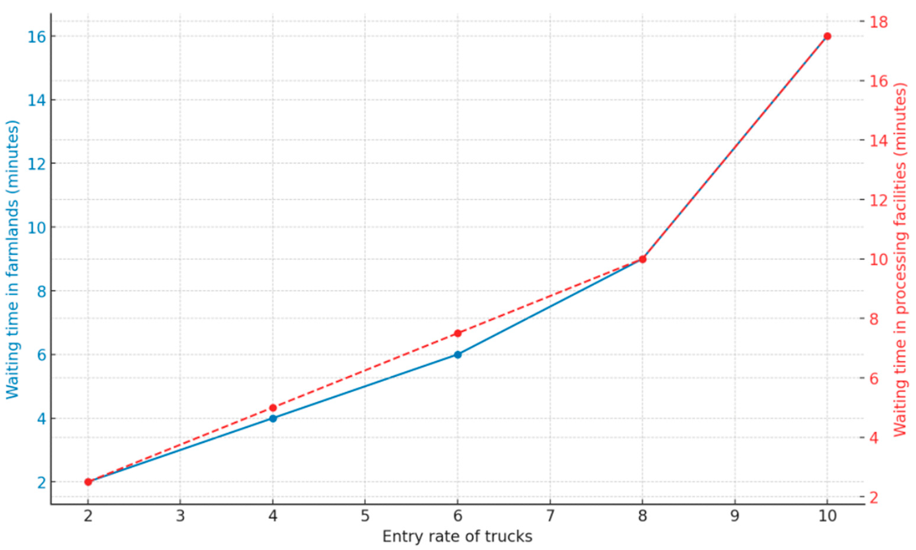
5.2.1. Changes in λ f s and λ l t s

Figure 2 illustrates the relationship between the entry rate of trucks and the waiting times in both farmlands and processing facilities. The left vertical axis represents the waiting time in farmlands (depicted by the solid blue line), while the right vertical axis represents the waiting time in processing facilities (depicted by the dashed red line). As the entry rate of trucks increases, both waiting times show a significant upward trend, indicating that higher entry rates lead to longer queues. This suggests that either the service rate or the number of servers in the queuing system should be increased to handle the growing demand more effectively. The dual-axis presentation allows for a clearer comparison between the two waiting times, facilitating a better understanding of the impact of entry rates on both types of facilities.

5.2.2. Changes in v a l p s

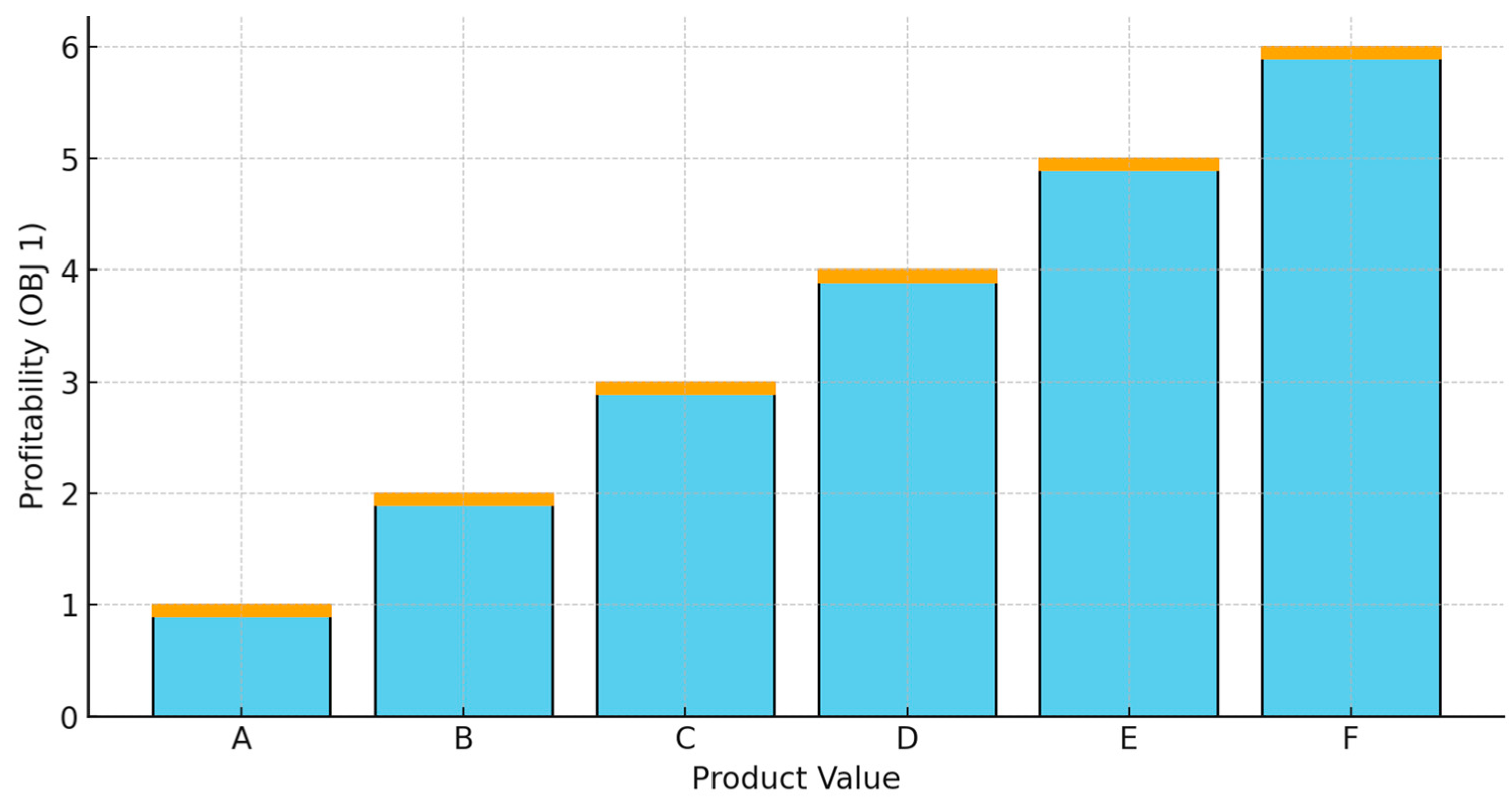
Increasing the value of each product will increase the overall profitability of the supply chain. The results are shown in Figure 3.
Figure 3 illustrates the relationship between the value of each product and the overall profitability of the supply chain, as measured by the first objective (objective 1). The trend observed in the graph indicates that as the product value increases, there is a corresponding rise in overall profitability. This positive correlation suggests that higher product value contributes significantly to enhancing the financial performance of the supply chain, underscoring the importance of optimizing product pricing and value within supply chain operations. The results clearly demonstrate that maximizing product value is a key factor in driving profitability in the modeled supply chain scenario.

5.2.3. Changes of o c t

Figure 4 shows that the supply chain will be distracted from its goal with increased operating costs.

5.3. Parameters Tuning

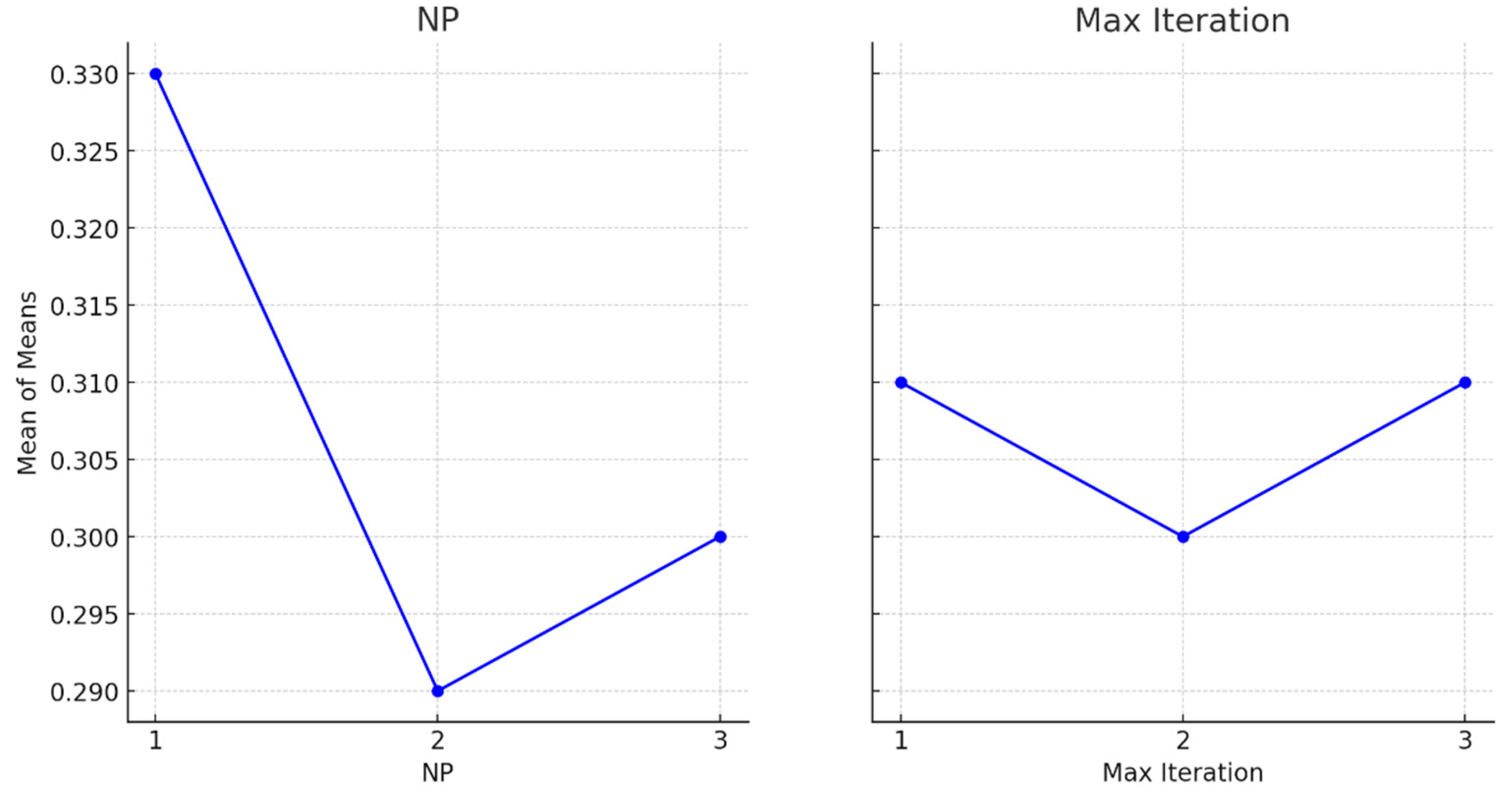
The Taguchi method is used as a suitable tool for setting the parameters of the GOA [26]. A three-level Taguchi design was applied to analyze the effects of essential GOA parameters, including population size and maximum number of iterations [27]. The results gained through performance of the Taguchi design for the large-scale problem in Minitab software are presented in Figure 5.

5.4. Results

To evaluate the algorithm’s capability, the results of the small and medium test problems with GAMS compared with the GOA are depicted in Table 5.
The results of solving the problem are shown in Table 5. The gap formula (45) is expressed as follows:
Gap rate = | Best sol − Test sol | × 100 / | Best sol |
The notation “n/a” means that there are no feasible solutions in the allowed time (5000 s) by GAMS solvers. The OBJ 1 unit is the currency ($). The OBJ 2 unit is hazardous unit emissions (H.u). The OBJ 3 unit is hours (h).
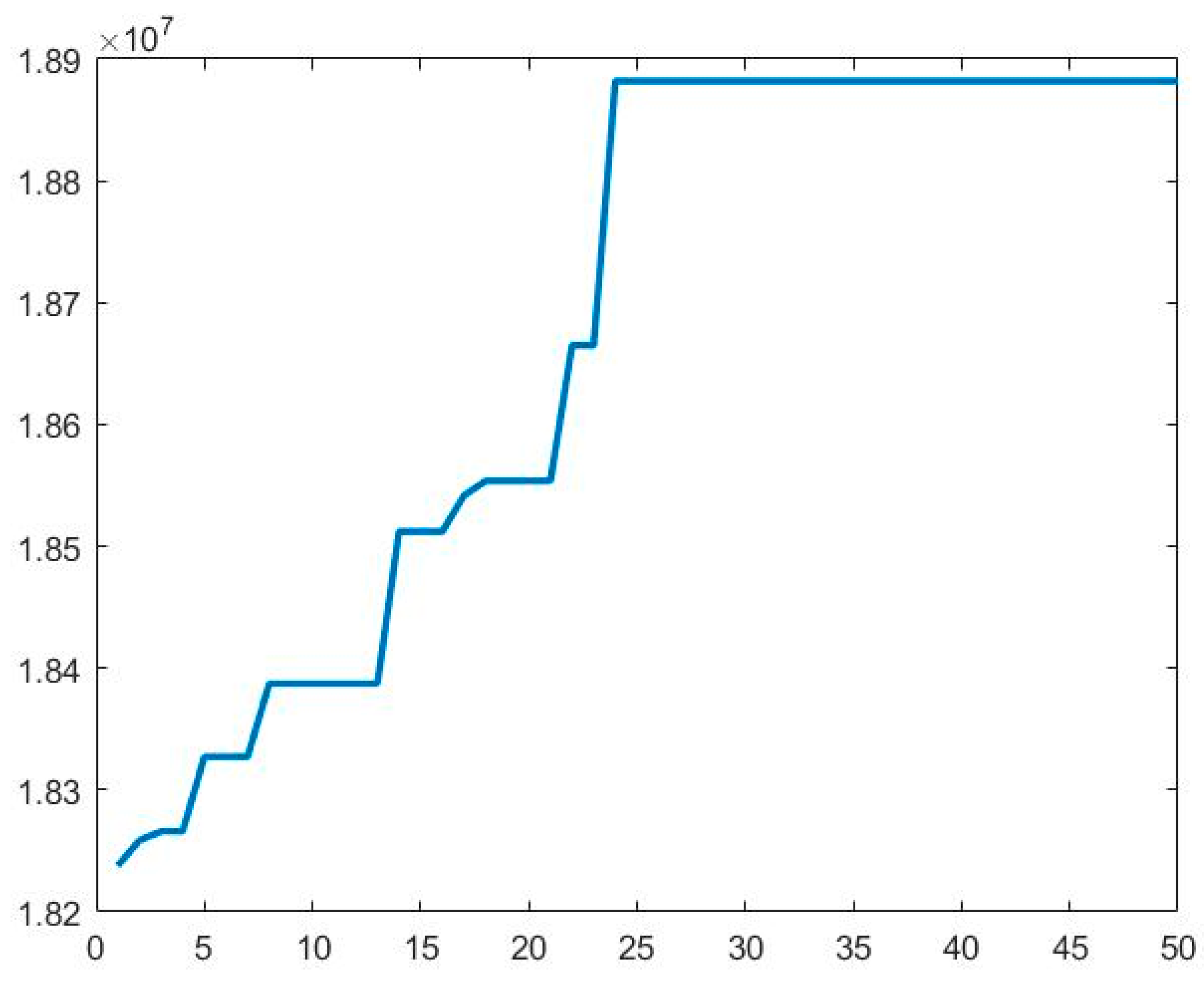
In Table 6 and Figure 6, the convergence graph of GOA for the first objective is depicted. According to the results, the outcomes of two optimization models, GAMS and GOA, across four problem instances, evaluating three primary objectives (OBJ 1, OBJ 2, and OBJ 3) and a linear programming objective (LP OBJ) are presented. Alongside these metrics, the percentage gap between the models’ results and CPU processing times are also reported. For problem number 2, GAMS and GOA show very close performances in OBJ 1, with values of 20.54 and 20.52, respectively, indicating a negligible difference in optimizing this metric. OBJ 2 presents a slight improvement in GOA, with values of 12.894 for GAMS and 12.98 for GOA. Similarly, for OBJ 3, the values are 14.71 for GAMS and 15.01 for GOA, again showing minor differences. The GAP percentages for OBJ 1, OBJ 2, and OBJ 3 are 0.097371%, 0.666977%, and 0.020394%, respectively, reflecting small discrepancies between the two models in these criteria. Regarding CPU time, GAMS and GOA recorded 40.78 and 24.56 s, respectively, highlighting GOA’s more efficient use of computational resources.
The chart illustrates the progression of a variable over time, increasing until it plateaus around the 35th point, possibly indicating that an optimal or stable state has been reached in the optimization process. This analysis demonstrates how different optimization approaches perform across various problems, assessing their efficiency and effectiveness in achieving near-optimal solutions within reasonable computational times.
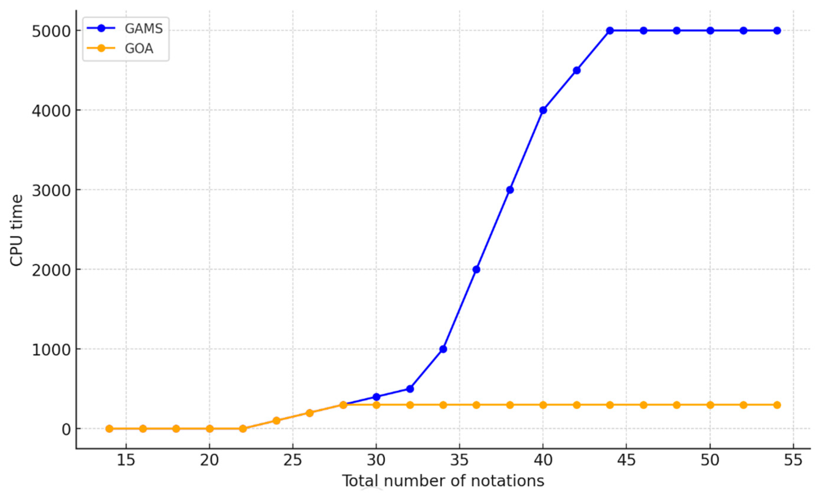
Figure 7 shows that the GOA can solve the problem logically when notations increase. Also, it can solve large-scale problems, which are impossible to solve with GAMS.

5.5. Case Study

This article primarily focuses on optimizing the rice supply chain, a crucial food ingredient for Iranian families. Given that rice production is predominantly in the north of Iran, optimizing this supply chain can significantly reduce total costs.
The locations of farmlands, nominated facility sites, and markets are initially shown in Figure 8. Processing facilities tend to be strategically placed closer to both the markets and farmlands to minimize transportation costs and improve efficiency. The proposed model considers a trade-off between supply chain costs, environmental impact, and drivers’ utility, ensuring that an optimal balance is maintained.
In the case study focused on Babol, the required number of processing facilities was determined to be six. Utilizing the collected data, our methodology involved identifying the best-nominated locations for these facilities. Initially, the distances between farmlands, facilities, and markets are detailed in Table 5. Subsequently, the algorithm processed this data to determine the optimal facility locations, with the results presented in Table 6. The number of scenarios corresponds to the number of nominated facility spots identified on the map. Table 7 and Table 8 illustrate the crucial trade-offs in supply chain management, emphasizing that optimal decisions need to balance cost, safety, and timeliness to meet diverse operational objectives effectively. Table 7 lists the parameters across various case studies that impact the setup and complexity of supply chain scenarios, including elements like farmlands, processing facilities, and markets.
Table 8 details the outcomes of specific scenarios analyzed for their impact on supply chain efficiency, measuring distance, cost, hazard units, and time. The results demonstrate significant variations across scenarios, reflecting how adjustments in parameters like distance affect cost and operational efficiency. For example, Scenario 1 shows moderate cost and hazard but longer time, while Scenario 6 achieves the shortest time but at the highest cost.

5.6. Sensitive Analysis

In this part, the sensitivity of the crucial parameters in the presented model is analyzed as follows:

5.6.1. Changes of c c f s and c l f l t

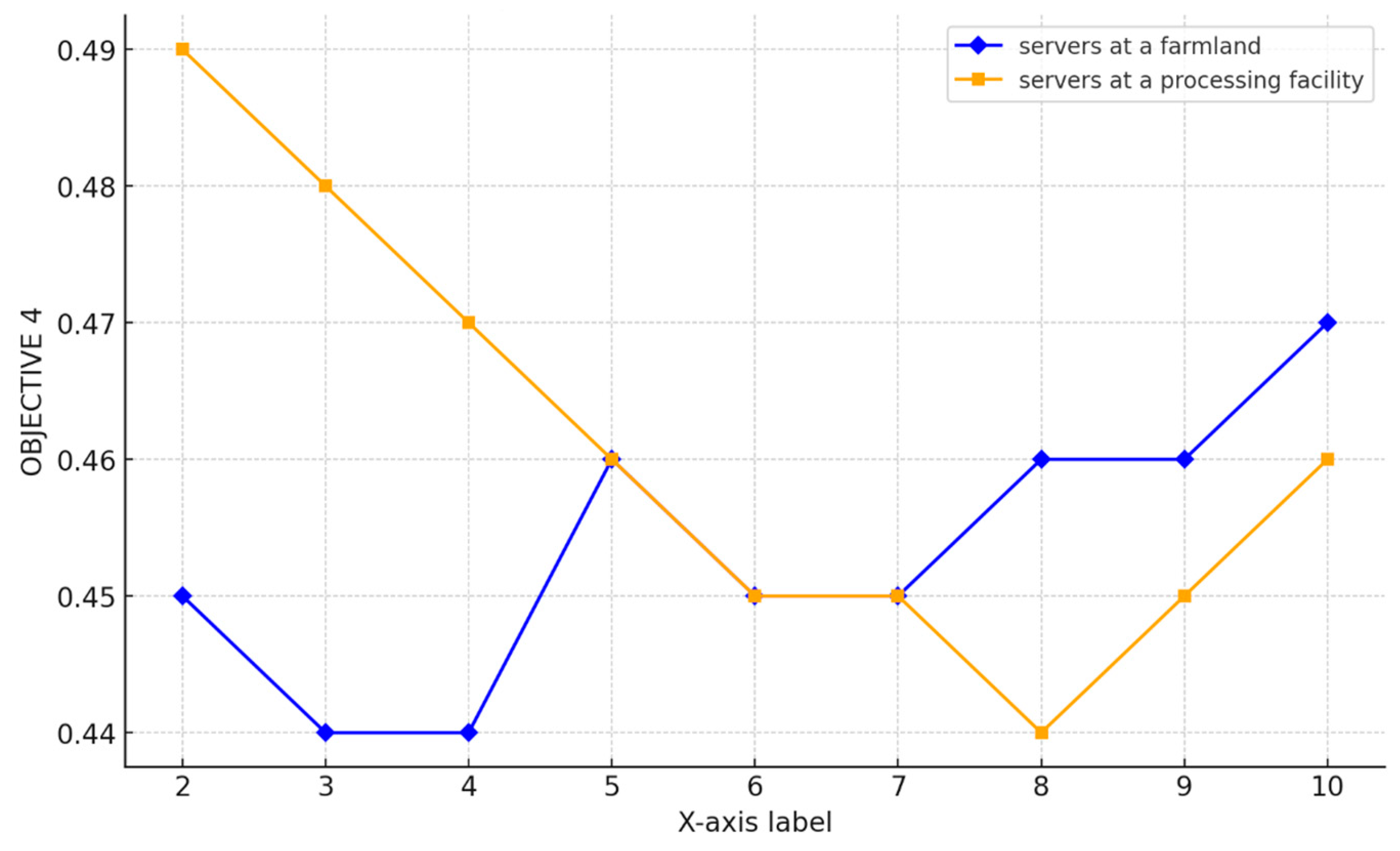
Regarding Table 9 and Figure 9, the best points that have the minimum objective function are obtained as ( c c f s = 4 ,   L P   O B J = 0.440 ) , ( c l f l t = 6 ,   L P   O B J = 0.438 ) for the number of servers at a farmland and at a facility.

5.6.2. Changes in W e i g h t 1 , W e i g h t 2 and W e i g h t 3

Regarding Table 10, which shows the impact of the weight of the objective function on the LP OBJ, the first objective has the most significant effect on LP OBJ.

5.6.3. Changes in d e m m p s

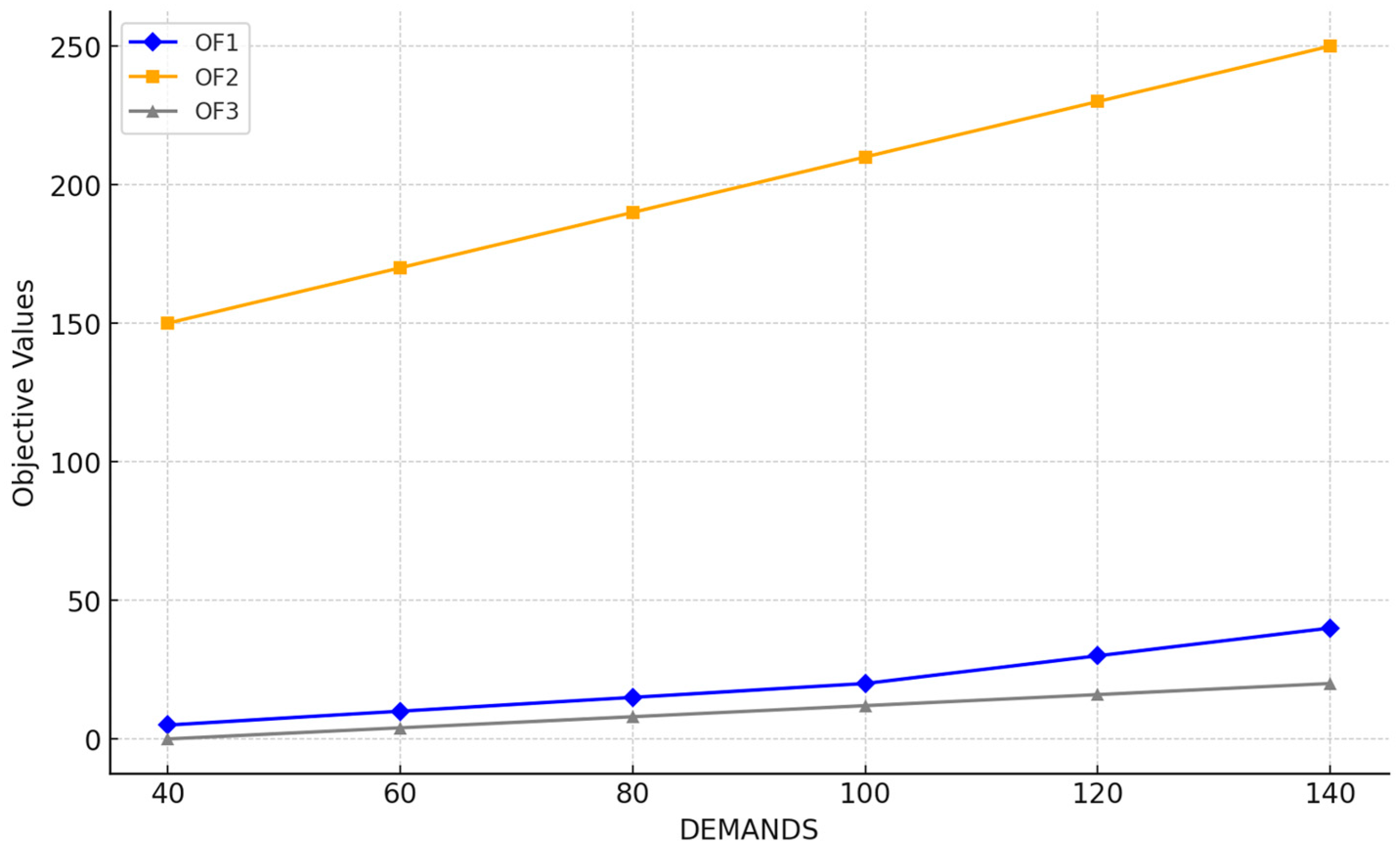
Table 11 and Figure 10 depict the impact of demand changes on the objective functions. The rate of increase in the first objective function ascends, but it gradually decreases in the second objective function. The third objective function is constant. As a result, managers should focus on profit and environmental aspects when the demand has an increasing rate.

5.6.4. Changes in Truck Features

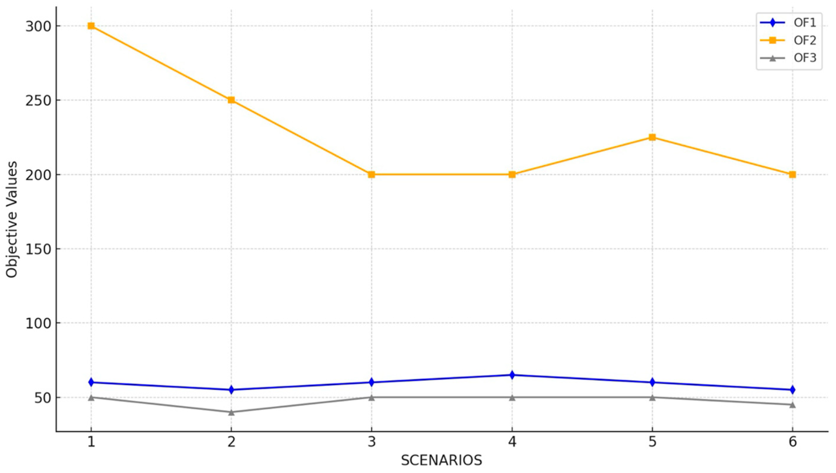
There are six different scenarios related to the available trucks’ condition, depicted in Table 12. The values of the objective functions related to each scenario are shown in Table 13 and Figure 11. The results help decision makers to decide according to their preferences.

6. Discussion

This study presents a novel approach to managing food supply chains by integrating M/M/C/K queuing systems with a location-allocation model, addressing critical gaps in the existing literature. Unlike previous studies that often focus on queuing issues in isolation, our research simultaneously considers multiple crops, intermediate products, seasonal time windows, and the environmental impact of transportation activities.
The implementation of M/M/C/K queuing systems in both farmlands and processing facilities demonstrates significant potential in reducing vehicle waiting times, a major source of operational inefficiency in food supply chains. By optimizing the number of servers and their allocation, our model effectively minimizes these delays, improving the overall flow of goods from farms to markets.
A key contribution of this study is the integration of the location-allocation problem within the queuing framework. By evaluating potential sites for processing facilities and determining optimal locations based on market demands, our model ensures a balanced distribution of resources. This enhances supply chain efficiency, ensures timely delivery of products to markets, and reduces waste.
Environmental sustainability is a crucial aspect of modern supply chain management. Our study emphasizes the reduction of CO2 emissions through optimized truck waiting times and route planning. The model significantly lowers the environmental footprint of the supply chain, aligning with increasing regulatory pressures and consumer demand for sustainable practices.
The case study in Babol, Iran, illustrates the practical applicability of the proposed model. The results highlight the model’s effectiveness in handling the complexities of real-world supply chains, providing actionable insight for supply chain managers. By maximizing total profit while minimizing environmental impact, the model offers both economic and ecological benefits.
Our detailed analysis of the rice supply chain in Babol shows significant impacts on cost reduction and efficiency. By focusing on regional data, we tailored solutions to the unique conditions of the area. These findings can serve as a foundation for future studies in other regions, offering comparative evaluations and broader applications. Additionally, the sensitivity analysis underscores the importance of considering research limitations and variables, demonstrating how changes in conditions can affect outcomes.
However, this study acknowledges certain limitations, such as the reliance on deterministic market demand, which may not fully capture real-world uncertainties. Future research could incorporate a stochastic demand model to better reflect market variability. While the case study provides valuable insight, further validation in different geographical and industrial contexts would strengthen the generalizability of the findings.
Also, we tested the proposed integrated multi-product, multi-period queuing location-allocation model using both small and large-scale scenarios to assess its effectiveness in optimizing a three-level food supply chain. The results demonstrate the model’s robustness and efficiency, particularly when utilizing the grasshopper optimization algorithm (GOA). In small and medium-sized problem instances, the GOA produced results comparable to those obtained using GAMS software, with minimal gaps in key objective functions. Specifically, the gap between GAMS and GOA in optimizing profitability (objective 1) ranged from 0.097% to 1.11%, indicating that GOA closely matches GAMS. For environmental impact (objective 2), the gap ranged from 0.172% to 1.83%, with GOA showing a slight advantage in reducing hazardous unit emissions. Additionally, the gap in minimizing waiting times (objective 3) was less than 0.027% across all instances, demonstrating that both methods provide similar results in this regard.
For large-scale problem instances, GAMS could not solve the problems within the allowed time (5000 s). However, GOA efficiently handled these cases, providing solutions with acceptable CPU times, ranging from 20.45 s for small instances to 64.78 s for larger ones. This highlights the efficiency of GOA in solving large-scale optimization problems within the supply chain context.
The impact of key parameters was also evaluated, revealing important insights. An increase in the truck arrival rate at farmlands and processing facilities directly increased the waiting time in queues, emphasizing the need for a balanced approach to service rates and the number of servers. Furthermore, a higher product value had a positive effect on overall supply chain profitability, with profits increasing from $29 million at 40,000 units to $49 million at 100,000 units. Conversely, increased operating costs led to a decrease in the overall objective function value, underscoring the importance of cost management in maintaining supply chain efficiency.
A case study focused on the rice supply chain in Babol identified optimal locations for six processing facilities, balancing trade-offs between supply chain costs, environmental impact, and driver utility. Scenario analysis revealed that Scenario 6 achieved the shortest time (11.75 h) but at the highest cost ($74.2 million), while Scenario 3 provided a balanced approach with moderate cost ($40.3 million), lower hazardous emissions (154,598 H.u.), and an acceptable waiting time (13.44 h).
The sensitivity analysis further demonstrated the model’s robustness to changes in key parameters, such as the number of servers at farmlands and facilities, and the weight assigned to each objective function. The analysis indicated that profitability had the most significant impact on the overall performance of the model. In conclusion, the results validate the applicability and effectiveness of the proposed model and the GOA in optimizing complex, large-scale supply chains, offering a powerful tool for decision makers to enhance supply chain efficiency and sustainability.
In comparison, the study by Perea-Lopez, Ydstie and Grossmann [10] also focused on supply chain optimization but used a model predictive control (MPC) strategy within a multiperiod MILP framework. Their approach considered the dynamic interactions within a supply chain and emphasized centralized versus decentralized management strategies. The results indicated that a centralized approach yielded up to 15% higher profits compared to decentralized methods, showcasing the importance of a holistic management strategy that considers all supply chain elements simultaneously.
While both studies address supply chain optimization, our research focuses on the queuing and location-allocation aspects combined with advanced heuristic algorithms, demonstrating efficiency across varying problem scales. By contrast, the study by Perea-Lopez, Ydstie and Grossmann [10] highlights the advantages of a centralized control approach in dynamic supply chains, particularly in improving profit margins by optimizing the entire supply chain simultaneously.
However, the case study does encounter certain limitations that warrant discussion. The scope of the data, primarily drawn from a single geographic region, may affect the generalizability of the conclusions. Future studies could expand the geographic scope to include diverse environments and market conditions, potentially offering a broader validation of the model’s effectiveness and adaptability.
Looking ahead, it is imperative that future research explores the integration of this model with advanced predictive analytics and real-time data processing technologies. Such advancements could enhance the model’s responsiveness to market dynamics and supply variability, providing a more dynamic and resilient supply chain framework. Additionally, further studies could investigate the socio-economic impacts of implementing such optimization models, particularly in terms of job creation, market competitiveness, and community sustainability.
The results of our case study in Babol demonstrate the practical applicability and robustness of the integrated M/M/C/K queuing and location-allocation model within a regional rice supply chain. This study not only reaffirms the model’s effectiveness in optimizing the flow of goods from farmlands to markets but also highlights its capability to adapt to and address the specific logistical challenges faced in rural settings. Particularly, the reduction in driver waiting times and improved facility utilization underscore the potential for significant cost savings and efficiency gains. Our findings also reveal critical insight into the environmental benefits of implementing such models. By optimizing routes and reducing idle times, the model significantly cuts down CO2 emissions, supporting sustainable practices within the supply chain. This aligns with current global priorities toward reducing environmental footprints and can serve as a compelling argument for the wider adoption of such models in similar contexts. This alignment underscores the importance of integrating sustainable practices in supply chain management, providing a robust framework for future developments in this field.
In conclusion, this research presents a comprehensive solution to the challenges faced by food supply chains, integrating queuing theory with a location-allocation model to enhance operational efficiency and environmental sustainability. The proposed model offers a robust framework for optimizing supply chain performance, with significant implications for both academic research and practical applications.

7. Conclusions

This study presents an innovative approach to managing food supply chains by integrating M/M/C/K queuing systems with a location-allocation model, addressing both operational efficiency and environmental sustainability. The proposed model considers multiple crops, intermediate products, and seasonal time windows, providing a realistic representation of agricultural supply chains. By optimizing vehicle waiting times and facility locations, the model enhances the flow of goods from farmlands to markets, ensuring timely delivery and preserving product quality.
Our research highlights several key contributions. First, the implementation of M/M/C/K queuing systems in both farmlands and processing facilities significantly reduces vehicle waiting times and improves overall supply chain efficiency. Second, the integration of a location-allocation problem with queuing systems ensures optimal facility placement and resource distribution. Third, the model emphasizes environmental sustainability, achieving significant reductions in CO2 emissions from transportation activities. Finally, the practical applicability of the model is demonstrated through a case study in Babol, Iran, illustrating its effectiveness in a real-world context.
The results indicate that the proposed model can maximize supply chain profit while minimizing environmental impact, providing a robust framework for supply chain optimization. This dual focus on economic and ecological objectives is essential in the current landscape of increasing regulatory pressures and consumer demand for sustainable practices.
However, there are some limitations to this study that should be acknowledged. The model’s reliance on deterministic market demand may not fully capture the uncertainties inherent in real-world supply chains. Additionally, the case study’s geographical and industrial context may limit the generalizability of the findings. Future validation across different regions and industries would help to strengthen the robustness of the model.
Future research should explore several avenues to build on the findings of this study. Incorporating a stochastic demand model could better reflect market variability and improve the model’s adaptability to real-world conditions. Additionally, expanding the model to include more complex supply chain dynamics and interactions would enhance its applicability. Investigating the integration of advanced technologies, such as blockchain for traceability and Internet of Things (IoT) for real-time monitoring, could further optimize supply chain operations and sustainability.
In conclusion, this research offers a comprehensive solution to the challenges faced by food supply chains, combining queuing theory and a location-allocation model to deliver substantial improvements in efficiency and sustainability. The findings have significant implications for both academic research and practical supply chain management, paving the way for more resilient and environmentally friendly supply chains.
In practical applications, certain products should not be transported together due to interactions that may accelerate spoilage. For instance, fruits such as bananas and avocados produce ethylene gas, which can accelerate the ripening or spoilage of other fruits and vegetables when stored in close proximity. This factor should be considered in the transportation planning phase to ensure the quality and longevity of the products. While the proposed M/M/C/K queuing model provides a robust framework for optimizing transportation and logistics, it is essential to incorporate these real-life limitations to enhance the model’s applicability and effectiveness in real-world scenarios.
This study lays the groundwork for incorporating M/M/C/K queuing systems in food supply chain management. Future research will focus on extending this model to cold chains in the food industry, where the perishability of products is a critical factor. Exploring the effects of temperature control, specialized storage conditions, and the separation of ethylene-producing fruits from other produce will be key areas of investigation. These enhancements aim to further improve the model’s practical relevance and effectiveness in managing perishable goods within the food supply chain.
Author Contributions

A.P.: Conceptualization, Methodology, Software, Visualization, Writing—original draft. H.Z.B.: Conceptualization, Methodology, Data curation, Writing—original draft. B.M.: Methodology, Software, Formal analysis, Writing—original draft M.M.M.: Writing—review & editing, Resources, Investigation, Validation, Project administration A.A.: Conceptualization, Methodology, Writing—review & editing, Validation, Supervision. All authors have read and agreed to the published version of the manuscript.

Funding

This research received no external funding.

Data Availability Statement

Data are contained within the article.

Conflicts of Interest

The authors declare no conflicts of interest.

References

  1. Muchhadiya, R.M.; Gohil, B.; Yadahalli, V.; Hm, A.U.R.; Siddiqua, A.; Khayum, A.; Behera, H.S.; Kumar, S. Feeding the world: Agronomic innovations to meet the challenges of a growing population. Int. J. Res. Agron. 2024, 7, 790–802. [Google Scholar] [CrossRef]
  2. Srivastava, S.K. Green supply-chain management: A state-of-the-art literature review. Int. J. Manag. Rev. 2007, 9, 53–80. [Google Scholar] [CrossRef]
  3. Sarkis, J. A boundaries and flows perspective of green supply chain management. Supply Chain Manag. Int. J. 2012, 17, 202–216. [Google Scholar] [CrossRef]
  4. Carter, C.R.; Rogers, D.S. A framework of sustainable supply chain management: Moving toward new theory. Int. J. Phys. Distrib. Logist. Manag. 2008, 38, 360–387. [Google Scholar] [CrossRef]
  5. Guinée, J.B.; Heijungs, R.; Huppes, G.; Zamagni, A.; Masoni, P.; Buonamici, R.; Ekvall, T.; Rydberg, T. Life cycle assessment: Past, present, and future. Environ. Sci. Technol. 2011, 45, 90–96. [Google Scholar] [CrossRef] [PubMed]
  6. Zipkin, P. Foundations of Inventory Management; Mcgraw-Hill: Irwin, NY, USA, 2000. [Google Scholar]
  7. Daganzo, C. Logistics Systems Analysis; Springer Science & Business Media: Cham, Switzerland, 2005. [Google Scholar]
  8. Gross, D. Fundamentals of Queueing Theory; John Wiley & Sons: Hoboken, NJ, USA, 2008. [Google Scholar]
  9. David, S.-L.; Philip, K.; Edith, S.-L. Designing and Managing the Supply Chain: Concepts Strategies and Case Studies; McGraw Hill: New York, NY, USA, 2000. [Google Scholar]
  10. Perea-López, E.; Ydstie, B.; Grossmann, I.E. A model predictive control strategy for supply chain optimization. Comput. Chem. Eng. 2003, 27, 1201–1218. [Google Scholar] [CrossRef]
  11. Kolahi-Randji, S.; Attari, M.Y.N.; Ala, A. Enhancement the performance of multi-level and multi-commodity in supply chain: A simulation approach. J. Soft Comput. Decis. Anal. 2023, 1, 18–38. [Google Scholar] [CrossRef]
  12. Buzacott, J.A.; Shanthikumar, J.G. Stochastic models of manufacturing systems; Prentice Hall International: London, UK, 1993. [Google Scholar]
  13. Use of simulation for improving the output rate: An industrial application. Available online: http://www.asim-fachtagung-spl.de/asim2008/papers/Proof_103-3c.pdf (accessed on 8 September 2024).
  14. Franceschetto, S.; Amico, C.; Brambilla, M.; Cigolini, R. Improving supply chain in the automotive industry with the right bill of material configuration. IEEE Eng. Manag. Rev. 2023, 51, 214–237. [Google Scholar] [CrossRef]
  15. Amellal, I.; Amellal, A.; Seghiouer, H.; Ech-Charrat, M.R. An integrated approach for modern supply chain management: Utilizing advanced machine learning models for sentiment analysis, demand forecasting, and probabilistic price prediction. Decis. Sci. Lett. 2024, 13, 237–248. [Google Scholar] [CrossRef]
  16. Mohtashami, Z.; Aghsami, A.; Jolai, F. A green closed loop supply chain design using queuing system for reducing environmental impact and energy consumption. J. Clean. Prod. 2019, 242, 118452. [Google Scholar] [CrossRef]
  17. Masoumi, M.; Aghsami, A.; Alipour-Vaezi, M.; Jolai, F.; Esmailifar, B. An M/M/C/K queueing system in an inventory routing problem considering congestion and response time for post-disaster humanitarian relief: A case study. J. Humanit. Logist. Supply Chain Manag. 2022, 12, 182–219. [Google Scholar] [CrossRef]
  18. Aghsami, A.; Abazari, S.R.; Bakhshi, A.; Yazdani, M.A.; Jolai, S.; Jolai, F. A meta-heuristic optimization for a novel mathematical model for minimizing costs and maximizing donor satisfaction in blood supply chains with finite capacity queueing systems. Health Anal. 2023, 3, 100136. [Google Scholar] [CrossRef]
  19. Karamipour, M.; Kermani, M.A.M.A. Presenting a mathematical model of blood supply chain considering the efficiency of collection centers and development of metaheuristic algorithm in M/M/C/K queuing system. Cereb. Cortex 2024, 34, bhae012. [Google Scholar] [CrossRef] [PubMed]
  20. Abbaspour, S.; Aghsami, A.; Jolai, F.; Yazdani, M. An integrated queueing-inventory-routing problem in a green dual-channel supply chain considering pricing and delivery period: A case study of construction material supplier. J. Comput. Des. Eng. 2022, 9, 1917–1951. [Google Scholar] [CrossRef]
  21. Aghsami, A.; Samimi, Y.; Aghaei, A. An integrated Markovian queueing-inventory model in a single retailer-single supplier problem with imperfect quality and destructive testing acceptance sampling. Adv. Ind. Eng. 2021, 55, 367–401. [Google Scholar]
  22. Deghoum, K.; Gherbi, M.T.; Sultan, H.S.; Al-Tamimi, A.N.J.; Abed, A.M.; Abdullah, O.I.; Mechakra, H.; Boukhari, A. Optimization of small horizontal axis wind turbines based on aerodynamic, steady-state, and dynamic analyses. Appl. Syst. Innov. 2023, 6, 33. [Google Scholar] [CrossRef]
  23. Ceselli, A.; Felipe, Á.; Ortuño, M.T.; Righini, G.; Tirado, G. A branch-and-cut-and-price algorithm for the electric vehicle routing problem with multiple technologies. SN Oper. Res. Forum 2021, 2, 8. [Google Scholar] [CrossRef]
  24. Schulz, J. Applying Mathematical Optimization in Practice: A Note on Insights from MO Projects. In Operations Research Forum; Springer: Cham, Switzerland, 2021. [Google Scholar]
  25. Mirjalili, S.Z.; Saremi, S.; Faris, H.; Aljarah, I. Grasshopper optimization algorithm for multi-objective optimization problems. Appl. Intell. 2018, 48, 805–820. [Google Scholar] [CrossRef]
  26. Parr, W.C. Introduction to Quality Engineering: Designing Quality into Products and Processes; Taylor & Francis: Abingdon, UK, 1989. [Google Scholar]
  27. Vanpoucke, E.; Boyer, K.K.; Vereecke, A. Supply chain information flow strategies: An empirical taxonomy. Int. J. Oper. Prod. Manag. 2009, 29, 1213–1241. [Google Scholar] [CrossRef]
Figure 1. Stages and types of flows of goods considered in the case implementation.
Logistics 08 00091 g001
Figure 2. Combined analysis of entry rate of trucks vs. waiting times in farmlands and processing facilities.
Logistics 08 00091 g002
Figure 3. Product value vs. profitability (objective 1).
Logistics 08 00091 g003
Figure 4. Operation cost vs. LP OBJ.
Logistics 08 00091 g004
Figure 5. Analysis diagrams of GOA parameters based on Taguchi method.
Logistics 08 00091 g005
Figure 6. Convergence of GOA to the optimal solution for the large scale.
Logistics 08 00091 g006
Figure 7. Changes in CPU time according to the total number of notations.
Logistics 08 00091 g007
Figure 8. Spatial distribution of facilities and markets in Babol before and after pptimization.
Logistics 08 00091 g008
Figure 9. Sensitivity analysis by changing c c f s a n d   c l f l t .
Logistics 08 00091 g009
Figure 10. Changes in d e m m p s impact.
Logistics 08 00091 g010
Figure 11. The values of objective functions according to the scenarios.
Logistics 08 00091 g011
Table 1. Index sets of this study.
Index
f ϵ F Set of farmlands
p ϵ P Set of products
s ϵ S Set of seasons
t ϵ T Set of processing facility types
m ϵ M Set of Markets
c ϵ C Set of crops
l ϵ L Set of possible processing facility locations
a ϵ A Set of transformations
I P Set of intermediate products
n ϵ N Set of truck numbers at farm f
n ϵ N Set of truck numbers at the processing facility
Table 2. Parameters of this study.
Parameters
VALPSValue of product p in season s
OCTOperating costs of processing facility type t
t c p Transport costs of product p per ton per km
t c c Transport costs of crop c per ton per km
d r f l Distance between farm region f and processing facility location l
d l l l Distance between processing facility location l and location l
d m l m Distance between processing facility location l and market m
s u p f c s Rate of supply in farm region f of crop c in season s
d e m m p s Rate of demand of product p at market m in season s
p r e m p s Lower bound demand of market m for product p in season s
f c l t Fixed costs for opening a processing facility type t
c a p s Total capacity in season s
c f t p a Conversion factor for product p in transformation a in facility type t
c r t c a Converted fraction of crop c in transformation a in facility type t
c r t i a Converted fraction of intermediate crop i in transformation a in facility type t
e t l l n Transportation-related CO2-eq emissions and harmful gases for transporting from processing facility location l to location l by truck n per unit of distance
e t f l n Transportation-related CO2-eq emissions and harmful gases for transporting from farm region f to location l by truck n per unit of distance
e t l m n Transportation-related CO2-eq emissions and harmful gases for transporting from processing facility location l to market m by truck n per unit of distance
λ f s Arrival rate of trucks to the farm f in season s
c c f s Number of servers at farm f in season s
k f Capacity of queue at farm f in season s
λ l t s Arrival rate of trucks to the processing facility l of type t in season s
c l l t s Number of servers at processing facility l of type t in season s of type t
k l Capacity of queue at processing facility l of type t in season s
PCAmount of load in each truck in every route
UBLPMaximum number of workers to load and unload a truck
LBLPMinimum amount of products or crops that a worker should load and unload from a truck
VAverage speed of trucks
MA big number
A f Opration cost of a server in farmland f
B f Marginal cost of a server in farmland f
A l Operation cost of a server in process facility l
B l Marginal cost of a server in process facility l
Table 3. Variables of this study.
Auxiliary Variables
W f s Average time a truck spends in farm f in season s
W Q f s Average time a truck spends in the queue of farm f in season s
L f s Average number of Trucks in farm f in season s
L Q f s Average number of Trucks in the queue of farm f in season s
π 0 f s Probability that there will be no trucks in farm f in season s
π k f f s Probability that there will be exactly k f trucks in farm f in season s
λ f s ¯ Effective arrival rate of trucks to the farm f in season s
W l t s Average time a truck spends in processing facility l of type t in season s
W Q l t s Average time a truck spends in the queue of processing facility l of type t in season s
L l t s Average number of trucks in processing facility l of type t in season s
L Q l t s Average number of trucks in the queue of processing facility l of type t in season s
π 0 l t s Probability that there will be no trucks in processing facility l of type t in season s
π k l l t s Probability that there will be exactly k l trucks in processing facility l of type t in season s
λ l t s ¯ Effective arrival rate of trucks to the processing facility l of type t in season s
F μ f s Operation and inaction costs function of servers in farmland f
F μ l t s Operation and inaction costs function of servers in processing facility l
ρ f s Traffic intensity of farm f queue in season s
ρ l t s Traffic intensity of queue of processing facility l of type t in season s
Decision Variables
X f l t c s Rate of crop c transported from farm f to a processing facility at location l of type t in season s in time unit
Q l l t t p s Rate of product p transported a processing facility at location l of type t to facility l of type t in season s in unit time
Z l m t p s Rate of product p transported from a processing facility at location l of type t to market m in season s in unit time
Y l t Processing facility at location l of type t open or not (binary)
μ f s Rate of service at farm f in season s
μ l t s Rate of service at processing facility l of type t in season s
Table 4. Data generation of parameters.
ParameterValueParameterValue
valps$10 oct$2
t c p $0.01 t c c $0.03
d r f l Uniform (20, 30) Km d l l l Uniform (1, 5) Km
d m l m Uniform (10, 15) Km s u p f c s 1
d e m m p s 90,000 Units p r e m p s 80,000 Units
f c l t $150 c a p s 85,000
c f t p a Uniform (0.5, 1) c r t c a Uniform (0.1, 0.2)
c r t i a Uniform (0.6, 1) e t l l n Uniform (0.2, 0.5)
e t f l n Uniform (0.5, 0.9) e t l m n Uniform (0.6, 1.2)
Pc60 unitUblpUniform (3, 5)
lblpUniform (1, 2)VUniform (20, 50)
Table 5. Generating the notations.
Problem NumberScaleNotations
FCPLTMTotal Number of Notations
1Small22223314
232223315
323333317
433333318
533334420
6Medium45566733
745577735
856687739
956688740
1056688841
Table 6. Results of examples.
Problem NumberGAMSGOAGAP (%)CPU Time
OBJ 1 (106$) OBJ 2 (104 ∗ H.u)OBJ 3 (h)LP OBJOBJ 1OBJ 2OBJ 3LP OBJOBJ 1OBJ 2OBJ 3LP OBJGAMSGOA
118.253410.41213.98018.2110.4314.0300.2377640.1728770.003576030.7820.45
220.5412.89414.71020.5212.9815.0100.0973710.6669770.020394040.7824.56
321.2413.2417.04021.00413.3417.0801.1111110.7552870.0023470100.7845.36
425.8216.8718.94025.6417.0119.0100.6971340.8298760.0036950120.8756.4
530.7318.4619.97030.4518.79820.500.9111621.8309860.0265390180.964.78
(* the final value is rounded on the large scale).
Table 7. Parameters Affecting Supply Chain Setup and Complexity.
DatasetFPSLTMCN N
Case study43462342015
Table 8. Characteristics of the considered datasets.
Scenario d r f l (km) d l l l (km) d m l m ( k m ) O B J 1 O B J 2 O B J 3
1202.514$38,207,000156,672 H.u13.55 h
2222.512$52,605,000142,848 H.u12.83 h
321.52.613.7$40,364,000154,598 H.u13.44 h
4232.316$23,808,000170,496 H.u14.27 h
529517$16,605,000177,408 H.u14.63 h
63019$74,202,000122,112 H.u11.75 h
7262.419$2,194,000191,232 H.u15.35 h
8272.615.5$27,405,000167,040 H.u14.09 h
9262.716.7$18,767,000175,334 H.u14.52 h
1026219.5$−194,000211,968 H.u16.43 h
11241.517.1$15,883,000178,098 H.u14.67 h
1229811$59,802,000135,936 H.u12.47 h
Table 9. Sensitivity analysis by changing c c f s a n d   c l f l t .
c c f s L P O B J c l f l t L P O B J
20.44220.488
30.44430.462
40.44040.459
50.47650.443
60.45060.438
70.45170.439
80.45180.446
90.45290.452
100.457100.455
Table 10. Sensitivity analysis of weights.
w e i g h t 1 w e i g h t 2 w e i g h t 3 L P O B J
0010.040
0.70.20.10.041
0.60.400.179
0.350.150.50.283
0.50.30.20.318
0.10.10.80.377
Table 11. Changes in d e m m p s impact.
d e m m p s OBJ 1OBJ 2OBJ 3
40 K$29 m150 K H.u.13.6 h
50 K$30 m170 K H.u.13.8 h
60 K$32 m185 K H.u.14.2 h
70 K$38 m195 K H.u.14.5 h
80 K$41 m205 K H.u.14.7 h
90 K$45 m209 K H.u.14.8 h
100 K$49 m211 K H.u.15.1 h
Table 12. Different scenarios of the trucks available in the region.
ScenarioVPc t c p t c c e t l l n e t f l n e t l m n
120 km/h60$0.0090.0280.50.91.2
228 km/h52$0.0080.0220.40.81.1
330 km/h50$0.0140.0320.20.50.6
435 km/h65$ 0.020.0360.350.750.15
540 km/h60$0.0150.0310.40.70.8
650 km/h50$0.010.030.30.60.7
Table 13. The values of objective functions according to the scenarios.
ScenariosOBJ 1OBJ 2OBJ 3
1$80 m300 K H.u.43 h
2$62 m260 K H.u.35 h
3$60 m170 K H.u.33 h
4$85 m210 K H.u.28 h
5$70 m250 K H.u.25 h
6$64 m200 K H.u.15 h
Disclaimer/Publisher’s Note: The statements, opinions and data contained in all publications are solely those of the individual author(s) and contributor(s) and not of MDPI and/or the editor(s). MDPI and/or the editor(s) disclaim responsibility for any injury to people or property resulting from any ideas, methods, instructions or products referred to in the content.