
Adaptive Large Neighborhood Search Metaheuristic for the Capacitated Vehicle Routing Problem with Parcel Lockers


Abstract
:1. Introduction
2. Relevant Literature
2.1. The Multiple Time Windows Vehicle Routing Problem
2.2. The Vehicle Routing Problem with Roaming Delivery Locations
2.3. The Vehicle Routing Problem with Transshipment Facilities
2.4. The Capable Vehicle Routing Problem with Pickup and Alternative Delivery
2.5. The Vehicle Routing Problem with Delivery Options
3. Problem Description
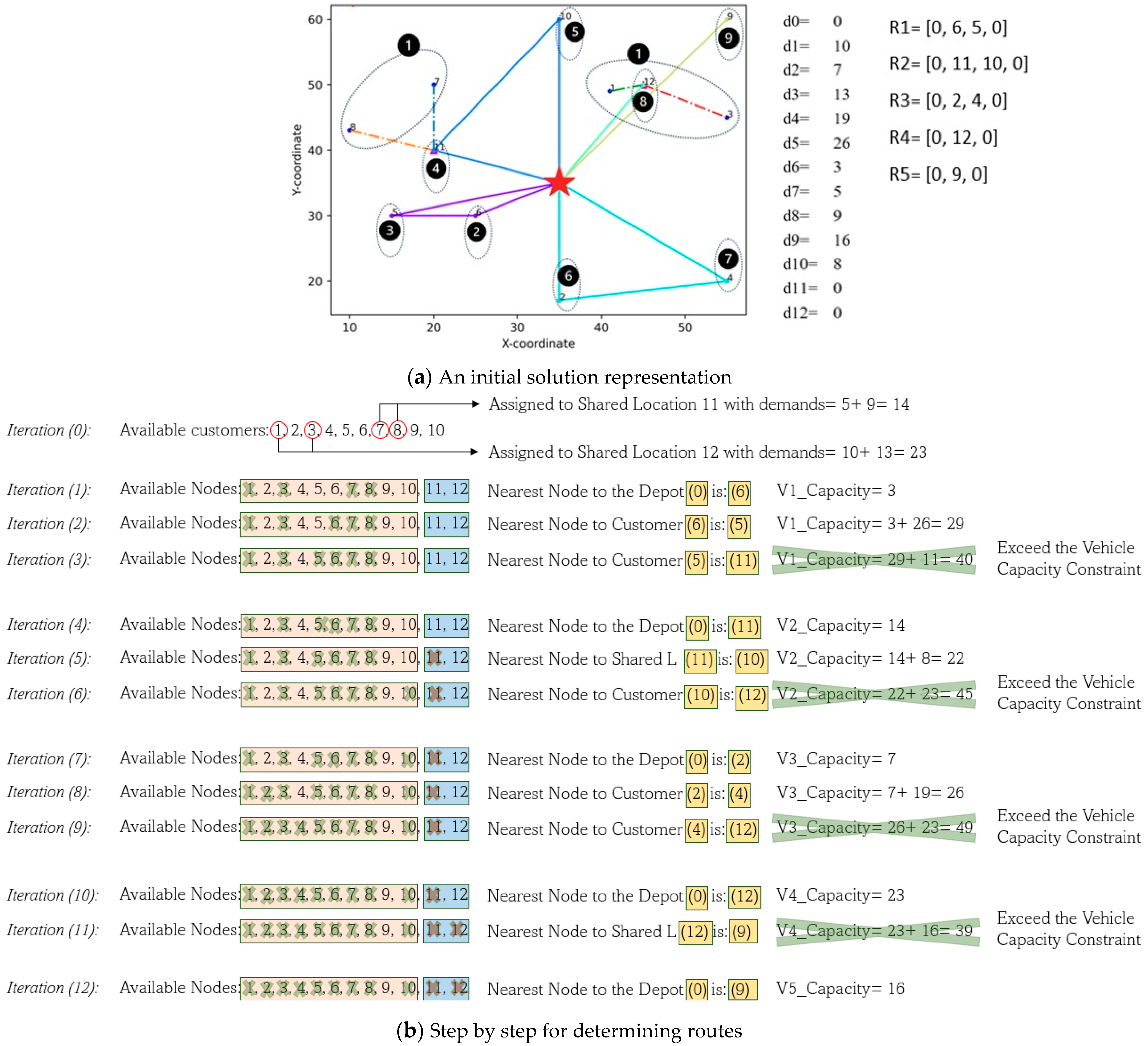
Capacity Synchronization
- Verification of the SDL list length: ensure that the number of customers associated with the SDL is less than or equal to the SDL capacity (in this example, three).
- Calculation of the SDL demand after incorporating the new customer: assess the total demand attributed to the SDL by considering the demands of all customers assigned to it, including the new addition.
- Recheck the vehicle capacity constraints if a customer is assigned to a SDL visited by that vehicle. This verification step is necessary as the SDL’s demands may differ from the initial check for this constraint.
4. Mathematical Model Formulation
5. Solution Using Adaptive Large Neighbourhood Search Approach
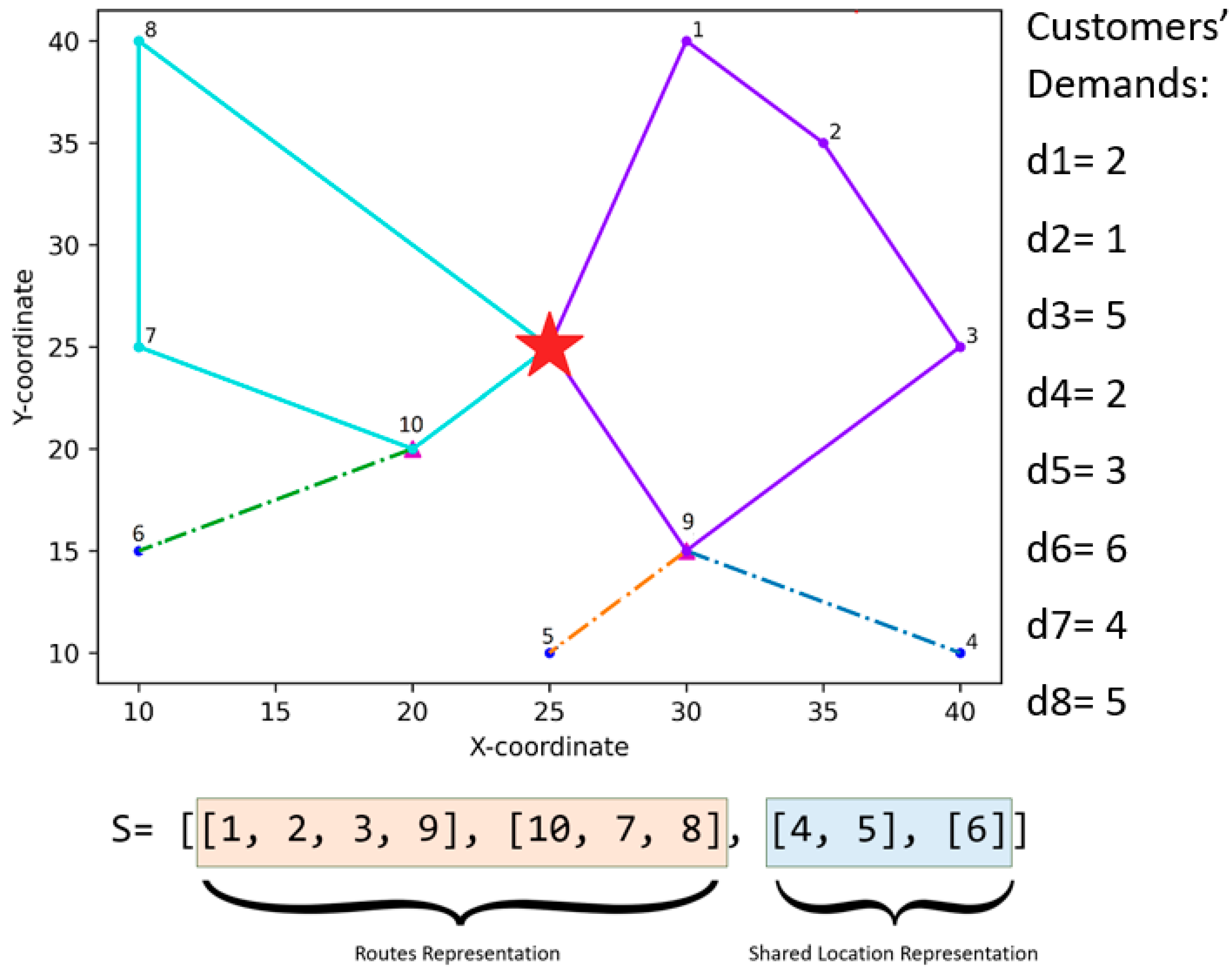
5.1. Solution Representation
| d[9] | = | d[4] + d[5] | = | 5 |
| d[10] | = | d[6] | = | 6 |
| Capacity [R1] | = | d[1] + d[2] + d[3] + d[9] | = | 13 |
| Capacity [R2] | = | d[10] + d[7] + d[8] | = | 15 |
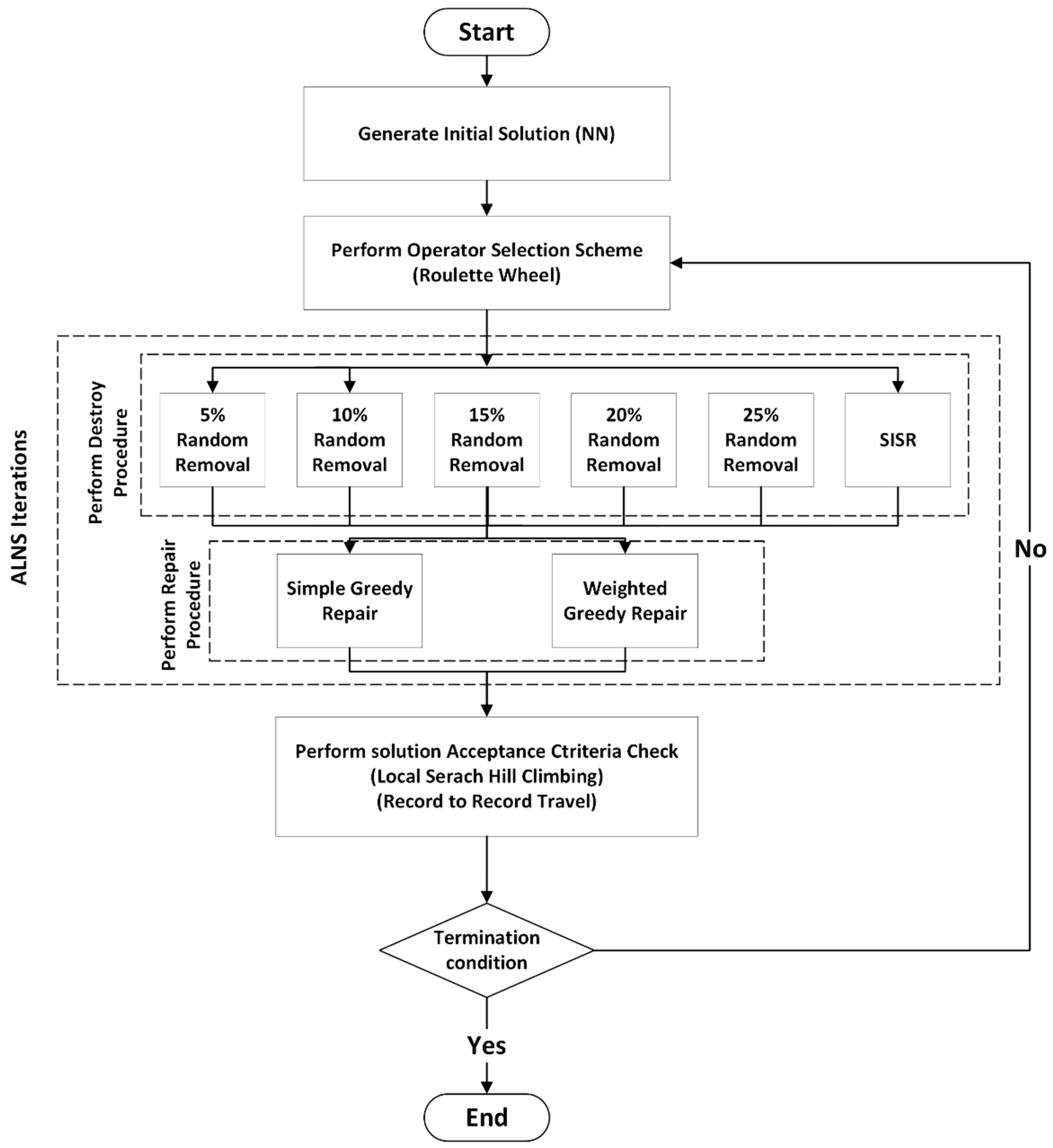
5.2. Initial Solution
5.3. Destroy Operators
5.3.1. Random Removal
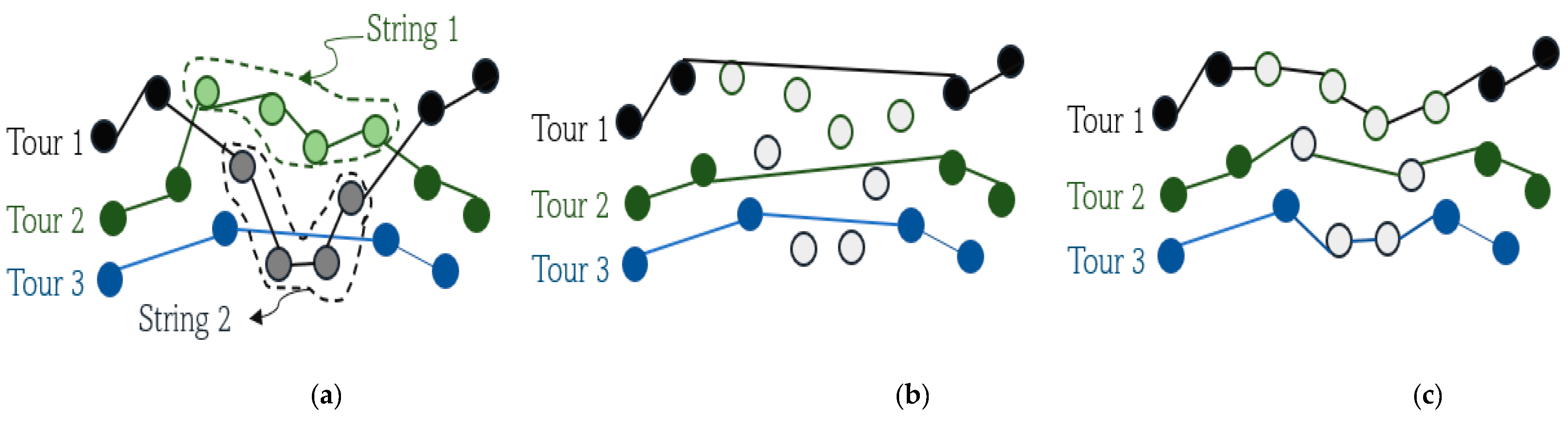
5.3.2. Slack Induction by String Removal (SISR)
5.4. Repair Operators
5.5. Operator Selection Scheme
- The candidate solution is a new global best.
- The candidate solution is better than the current solution, but not a global best.
- The candidate solution is accepted.
- The candidate solution is rejected.
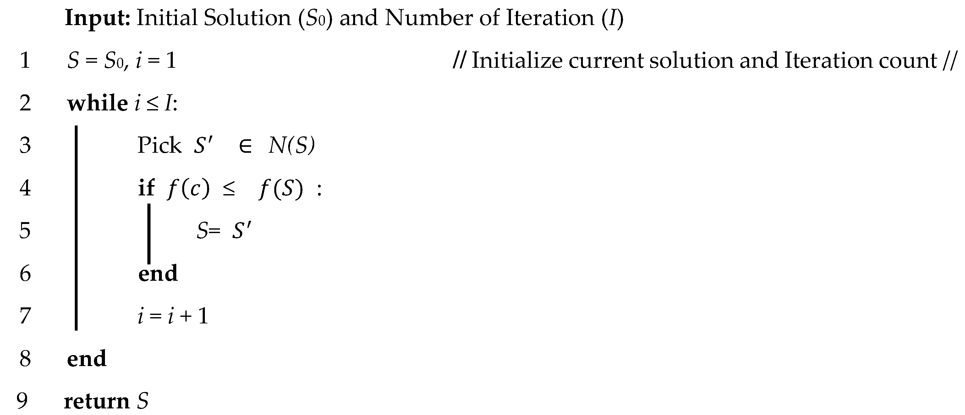
5.6. Acceptance Criteria
5.6.1. Hill Climbing
5.6.2. Record-to-Record Travel
6. Results and Discussion
6.1. Instances of the CVRPDO
6.2. Validation of the ALNS
6.3. Testing the Performance of the ALNS Parameters
6.4. Testing the Performance of the ALNS aginst Extended MIP Runs
6.5. Comprehensive Evaluation of the ALNS Performance
7. Conclusions
Author Contributions
Funding
Institutional Review Board Statement
Informed Consent Statement
Data Availability Statement
Acknowledgments
Conflicts of Interest
Appendix A. Detailed Results on the 1000 Customers Instances (MIP Runtimes: 5 h), and Detailed Results of the MIP with Runtimes: 3 h against ALNS for All Instances

| Instance | MIP | ALNS | ALNS | ALNS | ALNS | ALNS | |||||
|---|---|---|---|---|---|---|---|---|---|---|---|
| 5 h | 1 min | 2 min | 5 min | 7 min | 10 min | ||||||
| Sol | Sol | Gap | Sol | Gap | Sol | Gap | Sol | Gap | Sol | Gap | |
| C1_10 | 37,811 | 40,923 | 8% | 39,417 | 4% | 36,425 | −4% | 35,856 | −5% | 35,730 | −6% |
| C1_10 | 37,811 | 37,962 | 0% | 36,870 | −2% | 36,381 | −4% | 35,855 | −5% | 35,491 | −6% |
| C1_10 | 37,811 | 39,487 | 4% | 37,958 | 0% | 36,360 | −4% | 36,300 | −4% | 36,259 | −4% |
| C1_10 | 37,811 | 39,479 | 4% | 37,727 | 0% | 36,327 | −4% | 35,781 | −5% | 35,487 | −6% |
| C1_10 | 37,811 | 38,488 | 2% | 36,783 | −3% | 35,940 | −5% | 35,649 | −6% | 35,155 | −7% |
| Avg. | 37,811 | 39,267.8 | 4% | 37,751 | 0% | 36,286.6 | −4% | 35,888 | −5% | 35,624 | −6% |
| C2_10 | 39,753 | 39,920 | 0% | 38,711 | −3% | 36,916 | −7% | 36,411 | −8% | 35,652 | −10% |
| C2_10 | 39,753 | 43,640 | 10% | 38,406 | −3% | 36,584 | −8% | 35,933 | −10% | 35,460 | −11% |
| C2_10 | 39,753 | 40,867 | 3% | 38,973 | −2% | 37,622 | −5% | 36,754 | −8% | 36,183 | −9% |
| C2_10 | 39,753 | 44,202 | 11% | 41,441 | 4% | 38,032 | −4% | 36,332 | −9% | 35,706 | −10% |
| C2_10 | 39,753 | 38,786 | −2% | 37,307 | −6% | 35,406 | −11% | 35,317 | −11% | 35,241 | −11% |
| Avg. | 39,753 | 41,483 | 4% | 38,968 | −2% | 36,912 | −7% | 36,149 | −9% | 35,648 | −10% |
| R1_10 | 544,370 | 50,035 | −8% | 49,092 | −10% | 46,518 | −14% | 45,541 | −16% | 44,868 | −17% |
| R1_10 | 544,370 | 45,784 | −16% | 44,844 | −18% | 44,841 | −18% | 44,570 | −18% | 44,373 | −18% |
| R1_10 | 544,370 | 47,334 | −13% | 46,587 | −14% | 45,045 | −17% | 44,894 | −17% | 44,867 | −17% |
| R1_10 | 544,370 | 49,061 | −10% | 48,177 | −11% | 46,925 | −14% | 46,020 | −15% | 44,130 | −19% |
| R1_10 | 544,370 | 46,478 | −15% | 46,387 | −15% | 45,324 | −17% | 45,042 | −17% | 44,394 | −18% |
| Avg. | 544,370 | 47,738.4 | −12% | 47,017 | −14% | 45,731 | −16% | 45,213 | −17% | 44,526 | −18% |
| R2_10 | 52,413 | 48,892 | −7% | 46,499 | −11% | 45,399 | −13% | 44,820 | −14% | 44,658 | −15% |
| R2_10 | 52,413 | 49,090 | −6% | 48,056 | −8% | 46,409 | −11% | 45,553 | −13% | 44,487 | −15% |
| R2_10 | 52,413 | 48,322 | −8% | 47,554 | −9% | 45,233 | −14% | 44,611 | −15% | 44,540 | −15% |
| R2_10 | 52,413 | 50,280 | −4% | 48,412 | −8% | 45,280 | −14% | 44,001 | −16% | 43,853 | −16% |
| R2_10 | 52,413 | 47,067 | −10% | 45,839 | −13% | 44,896 | −14% | 44,359 | −15% | 44,164 | −16% |
| Avg. | 52,413 | 48,730.2 | −7% | 47,272 | −10% | 45,443 | −13% | 44,669 | −15% | 44,340 | −15% |
| RC1_10 | 53,400 | 45,553 | −15% | 44,756 | −16% | 42,905 | −20% | 42,426 | −21% | 42,122 | −21% |
| RC1_10 | 53,400 | 45,219 | −15% | 43,298 | −19% | 41,922 | −21% | 41,897 | −22% | 41,894 | −22% |
| RC1_10 | 53,400 | 46,389 | −13% | 44,957 | −16% | 43,542 | −18% | 43,040 | −19% | 43,040 | −19% |
| RC1_10 | 53,400 | 46,272 | −13% | 45,720 | −14% | 43,493 | −19% | 42,496 | −20% | 41,159 | −23% |
| RC1_10 | 53,400 | 44,922 | −16% | 44,480 | −17% | 43,236 | −19% | 42,960 | −20% | 42,421 | −21% |
| Avg. | 53,400 | 45,671 | −14% | 44,642.2 | −16% | 43,020 | −19% | 42,564 | −20% | 42,127 | −21% |
| Instance | MIP | ALNS | ALNS | ALNS | ALNS | ||||
|---|---|---|---|---|---|---|---|---|---|
| 3 h | 30 s | 60 s | 90 s | 120 s | |||||
| Sol | Sol | Gap | Sol | Gap | Sol | Gap | Sol | Gap | |
| C1_10 | 48,058 | 42,594 | −11% | 40,923 | −15% | 39,497 | −18% | 39,417 | −18% |
| C1_10 | 48,058 | 40,071 | −17% | 37,962 | −21% | 37,274 | −22% | 36,870 | −23% |
| C1_10 | 48,058 | 41,827 | −13% | 39,487 | −18% | 38,582 | −20% | 37,958 | −21% |
| C1_10 | 48,058 | 40,398 | −16% | 39,479 | −18% | 39,094 | −19% | 37,727 | −21% |
| C1_10 | 48,058 | 40,766 | −15% | 38,488 | −20% | 37,384 | −22% | 36,783 | −23% |
| Avg. | 48,058 | 41,131 | −14% | 39,268 | −18% | 38,366 | −20% | 37,751 | −21% |
| C2_10 | 47,728 | 41,088 | −14% | 39,920 | −16% | 39,433 | −17% | 38,711 | −19% |
| C2_10 | 47,728 | 44,683 | −6% | 43,640 | −9% | 40,504 | −15% | 38,406 | −20% |
| C2_10 | 47,728 | 43,333 | −9% | 40,867 | −14% | 39,516 | −17% | 38,973 | −18% |
| C2_10 | 47,728 | 45,648 | −4% | 44,202 | −7% | 42,416 | −11% | 41,441 | −13% |
| C2_10 | 47,728 | 40,816 | −14% | 38,786 | −19% | 38,311 | −20% | 37,307 | −22% |
| Avg. | 47,728 | 43,114 | −10% | 41,483 | −13% | 40,036 | −16% | 38,968 | −18% |
| R1_10 | 69,597 | 51,818 | −26% | 50,035 | −28% | 49,951 | −28% | 49,092 | −29% |
| R1_10 | 69,597 | 48,113 | −31% | 45,784 | −34% | 44,850 | −36% | 44,844 | −36% |
| R1_10 | 69,597 | 49,353 | −29% | 47,334 | −32% | 46,603 | −33% | 46,587 | −33% |
| R1_10 | 69,597 | 51,534 | −26% | 49,061 | −30% | 48,724 | −30% | 48,177 | −31% |
| R1_10 | 69,597 | 47,455 | −32% | 46,478 | −33% | 46,478 | −33% | 46,387 | −33% |
| Avg. | 69,597 | 49,655 | −29% | 47,738 | −31% | 47,321 | −32% | 47,017 | −32% |
| R2_10 | 69,010 | 51,342 | −26% | 48,892 | −29% | 47,909 | −31% | 46,499 | −33% |
| R2_10 | 69,010 | 51,240 | −26% | 49,090 | −29% | 48,656 | −29% | 48,056 | −30% |
| R2_10 | 69,010 | 50,067 | −27% | 48,322 | −30% | 47,856 | −31% | 47,554 | −31% |
| R2_10 | 69,010 | 51,422 | −25% | 50,280 | −27% | 49,384 | −28% | 48,412 | −30% |
| R2_10 | 69,010 | 50,261 | −27% | 47,067 | −32% | 46,100 | −33% | 45,839 | −34% |
| Avg. | 69,010 | 50,866 | −26% | 48,730 | −29% | 47,981 | −30% | 47,272 | −31% |
| RC1_10 | 55,882 | 47,124 | −16% | 45,553 | −18% | 44,756 | −20% | 44,756 | −20% |
| RC1_10 | 55,882 | 46,869 | −16% | 45,219 | −19% | 43,308 | −23% | 43,298 | −23% |
| RC1_10 | 55,882 | 47,239 | −15% | 46,389 | −17% | 45,117 | −19% | 44,957 | −20% |
| RC1_10 | 55,882 | 48,463 | −13% | 46,272 | −17% | 45,762 | −18% | 45,720 | −18% |
| RC1_10 | 55,882 | 45,547 | −18% | 44,922 | −20% | 44,570 | −20% | 44,480 | −20% |
| Avg. | 55,882 | 47,048 | −16% | 45,671 | −18% | 44,703 | −20% | 44,642 | −20% |
| Instance | MIP | ALNS | ALNS | ALNS | ALNS | ||||
|---|---|---|---|---|---|---|---|---|---|
| 3 h | 30 s | 60 s | 90 s | 120 s | |||||
| Sol | Sol | Gap | Sol | Gap | Sol | Gap | Sol | Gap | |
| C1_8 | 43,489 | 27,736 | −36% | 27,385 | −37% | 27,301 | −37% | 26,858 | −38% |
| C1_8 | 43,489 | 26,271 | −40% | 26,165 | −40% | 26,028 | −40% | 26,013 | −40% |
| C1_8 | 43,489 | 27,484 | −37% | 26,444 | −39% | 25,841 | −41% | 25,749 | −41% |
| C1_8 | 43,489 | 28,887 | −34% | 28,256 | −35% | 28,256 | −35% | 27,625 | −36% |
| C1_8 | 43,489 | 29,088 | −33% | 28,144 | −35% | 27,028 | −38% | 26,984 | −38% |
| Avg. | 43,489 | 27,893 | −36% | 27,279 | −37% | 26,891 | −38% | 26,646 | −39% |
| C2_8 | 40,022 | 30,205 | −25% | 29,328 | −27% | 29,328 | −27% | 28,427 | −29% |
| C2_8 | 40,022 | 30,499 | −24% | 29,197 | −27% | 28,257 | −29% | 28,216 | −29% |
| C2_8 | 40,022 | 30,158 | −25% | 28,652 | −28% | 28,212 | −30% | 27,889 | −30% |
| C2_8 | 40,022 | 30,639 | −23% | 29,643 | −26% | 28,467 | −29% | 28,430 | −29% |
| C2_8 | 40,022 | 31,245 | −22% | 29,828 | −25% | 29,584 | −26% | 29,150 | −27% |
| Avg. | 40,022 | 30,549 | −24% | 29,330 | −27% | 28,770 | −28% | 28,422 | −29% |
| R1_8 | 49,105 | 36,555 | −26% | 35,621 | −27% | 34,635 | −29% | 34,074 | −31% |
| R1_8 | 49,105 | 34,981 | −29% | 33,541 | −32% | 33,525 | −32% | 33,097 | −33% |
| R1_8 | 49,105 | 34,765 | −29% | 34,135 | −30% | 32,547 | −34% | 32,511 | −34% |
| R1_8 | 49,105 | 36,836 | −25% | 35,214 | −28% | 34,310 | −30% | 32,992 | −33% |
| R1_8 | 49,105 | 36,168 | −26% | 35,250 | −28% | 34,900 | −29% | 34,778 | −29% |
| Avg. | 49,105 | 35,861 | −27% | 34,752 | −29% | 33,983 | −31% | 33,490 | −32% |
| R2_8 | 43,725 | 35,637 | −18% | 35,559 | −19% | 34,864 | −20% | 34,789 | −20% |
| R2_8 | 43,725 | 35,808 | −18% | 35,344 | −19% | 34,050 | −22% | 33,672 | −23% |
| R2_8 | 43,725 | 35,571 | −19% | 35,196 | −20% | 34,764 | −20% | 34,293 | −22% |
| R2_8 | 43,725 | 34,261 | −22% | 33,483 | −23% | 32,736 | −25% | 32,295 | −26% |
| R2_8 | 43,725 | 34,378 | −21% | 34,234 | −22% | 33,795 | −23% | 33,559 | −23% |
| Avg. | 43,725 | 35,131 | −20% | 34,763 | −20% | 34,042 | −22% | 33,722 | −23% |
| RC1_8 | 45,585 | 34,801 | −24% | 32,790 | −28% | 32,419 | −29% | 32,419 | −29% |
| RC1_8 | 45,585 | 34,494 | −24% | 33,618 | −26% | 33,114 | −27% | 33,007 | −28% |
| RC1_8 | 45,585 | 36,142 | −21% | 35,434 | −22% | 34,903 | −23% | 34,621 | −24% |
| RC1_8 | 45,585 | 37,390 | −18% | 36,397 | −20% | 36,033 | −21% | 35,729 | −22% |
| RC1_8 | 45,585 | 35,289 | −23% | 34,956 | −23% | 34,225 | −25% | 33,260 | −27% |
| Avg. | 45,585 | 35,623 | −22% | 34,639 | −24% | 34,139 | −25% | 33,807 | −26% |
| Instance | MIP | ALNS | ALNS | ALNS | ALNS | ||||
|---|---|---|---|---|---|---|---|---|---|
| 3 h | 30 s | 60 s | 90 s | 120 s | |||||
| Sol | Sol | Gap | Sol | Gap | Sol | Gap | Sol | Gap | |
| C1_6 | 17,706 | 18,747 | 6% | 18,435 | 4% | 18,256 | 3% | 18,246 | 3% |
| C1_6 | 17,706 | 18,132 | 2% | 18,044 | 2% | 17,369 | −2% | 17,311 | −2% |
| C1_6 | 17,706 | 19,584 | 11% | 18,574 | 5% | 18,476 | 4% | 18,287 | 3% |
| C1_6 | 17,706 | 19,052 | 8% | 18,792 | 6% | 18,508 | 5% | 17,999 | 2% |
| C1_6 | 17,706 | 18,794 | 6% | 18,414 | 4% | 18,091 | 2% | 17,577 | −1% |
| Avg. | 17,706 | 18,862 | 7% | 18,452 | 4% | 18,140 | 2% | 17,884 | 1% |
| C2_6 | 21,190 | 21,737 | 3% | 21,384 | 1% | 20,814 | −2% | 20,575 | −3% |
| C2_6 | 21,190 | 21,756 | 3% | 20,949 | −1% | 19,260 | −9% | 19,134 | −10% |
| C2_6 | 21,190 | 22,000 | 4% | 20,954 | −1% | 20,764 | −2% | 20,455 | −3% |
| C2_6 | 21,190 | 21,459 | 1% | 20,287 | −4% | 19,690 | −7% | 19,330 | −9% |
| C2_6 | 21,190 | 20,503 | −3% | 19,971 | −6% | 19,147 | −10% | 18,822 | −11% |
| Avg. | 21,190 | 21,491 | 1% | 20,709 | −2% | 19,935 | −6% | 19,663 | −7% |
| R1_6 | 22,780 | 21,915 | −4% | 21,646 | −5% | 21,104 | −7% | 21,095 | −7% |
| R1_6 | 22,780 | 21,714 | −5% | 21,225 | −7% | 21,141 | −7% | 20,783 | −9% |
| R1_6 | 22,780 | 21,769 | −4% | 21,516 | −6% | 21,224 | −7% | 20,890 | −8% |
| R1_6 | 22,780 | 20,856 | −8% | 20,561 | −10% | 20,515 | −10% | 20,497 | −10% |
| R1_6 | 22,780 | 21,034 | −8% | 20,412 | −10% | 20,381 | −11% | 20,381 | −11% |
| Avg. | 22,780 | 21,458 | −6% | 21,072 | −7% | 20,873 | −8% | 20,729 | −9% |
| R2_6 | 23,286 | 21,662 | −7% | 21,384 | −8% | 20,991 | −10% | 20,767 | −11% |
| R2_6 | 23,286 | 22,179 | −5% | 21,596 | −7% | 21,567 | −7% | 21,520 | −8% |
| R2_6 | 23,286 | 22,196 | −5% | 21,666 | −7% | 21,337 | −8% | 21,061 | −10% |
| R2_6 | 23,286 | 21,486 | −8% | 21,032 | −10% | 20,938 | −10% | 20,475 | −12% |
| R2_6 | 23,286 | 21,140 | −9% | 20,369 | −13% | 20,182 | −13% | 20,156 | −13% |
| Avg. | 23,286 | 21,733 | −7% | 21,209 | −9% | 21,003 | −10% | 20,796 | −11% |
| RC1_6 | 20,978 | 20,694 | −1% | 20,676 | −1% | 20,053 | −4% | 19,757 | −6% |
| RC1_6 | 20,978 | 20,046 | −4% | 19,604 | −7% | 19,465 | −7% | 19,280 | −8% |
| RC1_6 | 20,978 | 20,003 | −5% | 19,882 | −5% | 19,845 | −5% | 19,748 | −6% |
| RC1_6 | 20,978 | 21,245 | 1% | 20,194 | −4% | 20,017 | −5% | 19,898 | −5% |
| RC1_6 | 20,978 | 19,635 | −6% | 18,999 | −9% | 18,711 | −11% | 18,276 | −13% |
| Avg. | 20,978 | 20,325 | −3% | 19,871 | −5% | 19,618 | −6% | 19,392 | −8% |
| Instance | MIP | ALNS | ALNS | ALNS | ALNS | ||||
|---|---|---|---|---|---|---|---|---|---|
| 3 h | 30 s | 60 s | 90 s | 120 s | |||||
| Sol | Sol | Gap | Sol | Gap | Sol | Gap | Sol | Gap | |
| C1_4 | 12,518 | 12,836 | 3% | 12,704 | 1% | 12,271 | −2% | 12,009 | −4% |
| C1_4 | 12,518 | 12,974 | 4% | 12,794 | 2% | 12,528 | 0% | 12,411 | −1% |
| C1_4 | 12,518 | 12,571 | 0% | 12,485 | 0% | 12,264 | −2% | 12,260 | −2% |
| C1_4 | 12,518 | 12,213 | −2% | 12,213 | −2% | 12,206 | −2% | 11,981 | −4% |
| C1_4 | 12,518 | 12,717 | 2% | 12,395 | −1% | 12,148 | −3% | 12,006 | −4% |
| Avg. | 12,518 | 12,662 | 1% | 12,518 | 0% | 12,283 | −2% | 12,133 | −3% |
| C2_4 | 12,523 | 12,714 | 2% | 12,402 | −1% | 12,318 | −2% | 12,310 | −2% |
| C2_4 | 12,523 | 12,984 | 4% | 12,575 | 0% | 12,364 | −1% | 12,237 | −2% |
| C2_4 | 12,523 | 12,653 | 1% | 12,129 | −3% | 12,090 | −3% | 12,054 | −4% |
| C2_4 | 12,523 | 12,756 | 2% | 12,290 | −2% | 12,190 | −3% | 12,190 | −3% |
| C2_4 | 12,523 | 12,378 | −1% | 12,321 | −2% | 12,298 | −2% | 12,298 | −2% |
| Avg. | 12,523 | 12,697 | 1% | 12,343 | −1% | 12,252 | −2% | 12,218 | −2% |
| R1_4 | 14,414 | 14,408 | 0% | 14,170 | −2% | 13,838 | −4% | 13,809 | −4% |
| R1_4 | 14,414 | 14,451 | 0% | 13,795 | −4% | 13,465 | −7% | 13,356 | −7% |
| R1_4 | 14,414 | 14,371 | 0% | 14,092 | −2% | 13,537 | −6% | 13,398 | −7% |
| R1_4 | 14,414 | 14,905 | 3% | 13,679 | −5% | 13,624 | −5% | 13,624 | −5% |
| R1_4 | 14,414 | 13,984 | −3% | 13,650 | −5% | 13,431 | −7% | 13,431 | −7% |
| Avg. | 14,414 | 14,424 | 0% | 13,877 | −4% | 13,579 | −6% | 13,524 | −6% |
| R2_4 | 14,490 | 14,766 | 2% | 14,619 | 1% | 14,510 | 0% | 14,407 | −1% |
| R2_4 | 14,490 | 14,120 | −3% | 13,773 | −5% | 13,545 | −7% | 13,330 | −8% |
| R2_4 | 14,490 | 14,701 | 1% | 13,590 | −6% | 13,590 | −6% | 13,590 | −6% |
| R2_4 | 14,490 | 14,591 | 1% | 14,096 | −3% | 14,004 | −3% | 13,991 | −3% |
| R2_4 | 14,490 | 15,014 | 4% | 14,448 | 0% | 14,277 | −1% | 14,261 | −2% |
| Avg. | 14,490 | 14,638 | 1% | 14,105 | −3% | 13,985 | −3% | 13,916 | −4% |
| RC1_4 | 14,034 | 13,632 | −3% | 13,070 | −7% | 13,070 | −7% | 12,989 | −7% |
| RC1_4 | 14,034 | 13,450 | −4% | 13,329 | −5% | 13,173 | −6% | 13,173 | −6% |
| RC1_4 | 14,034 | 14,595 | 4% | 14,351 | 2% | 13,459 | −4% | 13,122 | −6% |
| RC1_4 | 14,034 | 13,979 | 0% | 13,462 | −4% | 13,169 | −6% | 12,969 | −8% |
| RC1_4 | 14,034 | 13,399 | −5% | 13,295 | −5% | 13,184 | −6% | 12,876 | −8% |
| Avg. | 14,034 | 13,811 | −2% | 13,501 | −4% | 13,211 | −6% | 13,026 | −7% |
| Instance | MIP | ALNS | ALNS | ALNS | ALNS | ||||
|---|---|---|---|---|---|---|---|---|---|
| 3 h | 30 s | 60 s | 90 s | 120 s | |||||
| Sol | Sol | Gap | Sol | Gap | Sol | Gap | Sol | Gap | |
| C1_2 | 6757 | 7023 | 4% | 6840 | 1% | 6604 | −2% | 6537 | −3% |
| C1_2 | 6757 | 6681 | −1% | 6628 | −2% | 6609 | −2% | 6539 | −3% |
| C1_2 | 6757 | 6994 | 4% | 6594 | −2% | 6538 | −3% | 6520 | −4% |
| C1_2 | 6757 | 6955 | 3% | 6891 | 2% | 6581 | −3% | 6434 | −5% |
| C1_2 | 6757 | 6516 | −4% | 6441 | −5% | 6441 | −5% | 6414 | −5% |
| Avg. | 6757 | 6834 | 1% | 6679 | −1% | 6555 | −3% | 6489 | −4% |
| C2_2 | 6998 | 6778 | −3% | 6690 | −4% | 6685 | −4% | 6610 | −6% |
| C2_2 | 6998 | 6649 | −5% | 6621 | −5% | 6613 | −6% | 6613 | −6% |
| C2_2 | 6998 | 6772 | −3% | 6674 | −5% | 6569 | −6% | 6533 | −7% |
| C2_2 | 6998 | 6743 | −4% | 6723 | −4% | 6670 | −5% | 6616 | −5% |
| C2_2 | 6998 | 6728 | −4% | 6629 | −5% | 6593 | −6% | 6542 | −7% |
| Avg. | 6998 | 6734 | −4% | 6667 | −5% | 6626 | −5% | 6583 | −6% |
| R1_2 | 7735 | 7038 | −9% | 6993 | −10% | 6944 | −10% | 6913 | −11% |
| R1_2 | 7735 | 6974 | −10% | 6878 | −11% | 6878 | −11% | 6878 | −11% |
| R1_2 | 7735 | 7042 | −9% | 7029 | −9% | 7018 | −9% | 7006 | −9% |
| R1_2 | 7735 | 7212 | −7% | 7031 | −9% | 6972 | −10% | 6957 | −10% |
| R1_2 | 7735 | 7006 | −9% | 6932 | −10% | 6909 | −11% | 6831 | −12% |
| Avg. | 7735 | 7054 | −9% | 6973 | −10% | 6944 | −10% | 6917 | −11% |
| R2_2 | 7368 | 7297 | −1% | 7121 | −3% | 7088 | −4% | 7007 | −5% |
| R2_2 | 7368 | 7059 | −4% | 6967 | −5% | 6948 | −6% | 6935 | −6% |
| R2_2 | 7368 | 6946 | −6% | 6833 | −7% | 6783 | −8% | 6772 | −8% |
| R2_2 | 7368 | 7091 | −4% | 6868 | −7% | 6775 | −8% | 6769 | −8% |
| R2_2 | 7368 | 7169 | −3% | 7019 | −5% | 6962 | −6% | 6950 | −6% |
| Avg. | 7368 | 7112 | −3% | 6962 | −6% | 6911 | −6% | 6887 | −7% |
| RC1_2 | 6725 | 6859 | 2% | 6670 | −1% | 6603 | −2% | 6575 | −2% |
| RC1_2 | 6725 | 6656 | −1% | 6535 | −3% | 6526 | −3% | 6442 | −4% |
| RC1_2 | 6725 | 6491 | −3% | 6470 | −4% | 6470 | −4% | 6470 | −4% |
| RC1_2 | 6725 | 6806 | 1% | 6741 | 0% | 6693 | 0% | 6679 | −1% |
| RC1_2 | 6725 | 7085 | 5% | 6671 | −1% | 6671 | −1% | 6671 | −1% |
| Avg. | 6725 | 6779 | 1% | 6617 | −2% | 6593 | −2% | 6567 | −2% |
| Instance | MIP | ALNS | ALNS | ALNS | ALNS | ||||
|---|---|---|---|---|---|---|---|---|---|
| 3 h | 10 s | 20 s | 30 s | 40 s | |||||
| Sol | Sol | Gap | Sol | Gap | Sol | Gap | Sol | Gap | |
| C101 | 2390 | 2460 | 3% | 2405 | 1% | 2402 | 1% | 2402 | 1% |
| C101 | 2390 | 2489 | 4% | 2399 | 0% | 2396 | 0% | 2396 | 0% |
| C101 | 2390 | 2419 | 1% | 2412 | 1% | 2407 | 1% | 2407 | 1% |
| C101 | 2390 | 2411 | 1% | 2411 | 1% | 2411 | 1% | 2411 | 1% |
| C101 | 2390 | 2550 | 7% | 2399 | 0% | 2399 | 0% | 2398 | 0% |
| Avg. | 2390 | 2466 | 3% | 2405 | 1% | 2403 | 1% | 2403 | 1% |
| C201 | 2615 | 2754 | 5% | 2723 | 4% | 2701 | 3% | 2701 | 3% |
| C201 | 2615 | 2906 | 11% | 2875 | 10% | 2747 | 5% | 2741 | 5% |
| C201 | 2615 | 2759 | 6% | 2746 | 5% | 2737 | 5% | 2728 | 4% |
| C201 | 2615 | 2898 | 11% | 2803 | 7% | 2778 | 6% | 2762 | 6% |
| C201 | 2615 | 2734 | 5% | 2637 | 1% | 2636 | 1% | 2636 | 1% |
| Avg. | 2615 | 2810 | 7% | 2757 | 5% | 2720 | 4% | 2714 | 4% |
| R101 | 2274 | 2387 | 5% | 2340 | 3% | 2280 | 0% | 2280 | 0% |
| R101 | 2274 | 2387 | 5% | 2340 | 3% | 2280 | 0% | 2280 | 0% |
| R101 | 2274 | 2292 | 1% | 2290 | 1% | 2290 | 1% | 2290 | 1% |
| R101 | 2274 | 2387 | 5% | 2340 | 3% | 2280 | 0% | 2280 | 0% |
| R101 | 2274 | 2292 | 1% | 2290 | 1% | 2290 | 1% | 2290 | 1% |
| Avg. | 2274 | 2349 | 3% | 2320 | 2% | 2284 | 0% | 2284 | 0% |
| R201 | 2192 | 2268 | 3% | 2189 | 0% | 2183 | 0% | 2166 | −1% |
| R201 | 2192 | 2161 | −1% | 2161 | −1% | 2157 | −2% | 2152 | −2% |
| R201 | 2192 | 2194 | 0% | 2178 | −1% | 2167 | −1% | 2167 | −1% |
| R201 | 2192 | 2186 | 0% | 2186 | 0% | 2185 | 0% | 2176 | −1% |
| R201 | 2192 | 2212 | 1% | 2194 | 0% | 2175 | −1% | 2175 | −1% |
| Avg. | 2192 | 2204 | 1% | 2182 | 0% | 2173 | −1% | 2167 | −1% |
| RC101 | 2904 | 3258 | 12% | 3233 | 11% | 3218 | 11% | 3109 | 7% |
| RC101 | 2904 | 3142 | 8% | 3087 | 6% | 3027 | 4% | 3017 | 4% |
| RC101 | 2904 | 3156 | 9% | 3022 | 4% | 3005 | 3% | 2987 | 3% |
| RC101 | 2904 | 3087 | 6% | 3087 | 6% | 3045 | 5% | 3016 | 4% |
| RC101 | 2904 | 3108 | 7% | 3022 | 4% | 2977 | 3% | 2976 | 2% |
| Avg. | 2904 | 3150 | 8% | 3090 | 6% | 3054 | 5% | 3021 | 4% |
References
- Janjevic, M.; Winkenbach, M. Characterizing urban last-mile distribution strategies in mature and emerging e-commerce markets. Transp. Res. Part A Policy Pract. 2020, 133, 164–196. [Google Scholar] [CrossRef]
- Mancini, S.; Gansterer, M. Vehicle routing with private and shared delivery locations. Comput. Oper. Res. 2021, 133, 105361. [Google Scholar] [CrossRef]
- Saker, A.; Iijima, J.; Ali, I.; Eltawil, A. Capacitated Vehicle Routing Problem with Delivery Options: Private or Shared Location. In Proceedings of the ICIEA 2023, the 10th International Conference on Industrial Engineering and Applications, Phuket, Thailand, 4–6 April 2023. [Google Scholar]
- Reyes, D.; Savelsbergh, M.; Toriello, A. Vehicle routing with roaming delivery locations. Transp. Res. Part C Emerg. Technol. 2017, 80, 71–91. [Google Scholar] [CrossRef]
- Zhou, L.; Wang, X.; Ni, L.; Lin, Y. Location-routing problem with simultaneous home delivery and customer’s pickup for city distribution of online shopping purchases. Sustainability 2016, 8, 828. [Google Scholar] [CrossRef]
- Deutsch, Y.; Golany, B. A parcel locker network as a solution to the logistics last mile problem. Int. J. Prod. Res. 2018, 56, 251–261. [Google Scholar] [CrossRef]
- Vakulenko, Y.; Hellström, D.; Hjort, K. What’s in the parcel locker? Exploring customer value in e-commerce last mile delivery. J. Bus. Res. 2018, 88, 421–427. [Google Scholar] [CrossRef]
- Parcu, P.L.; Brennan, T.; Glass, V. The Changing Postal Environment; Springer: Berlin/Heidelberg, Germany, 2020. [Google Scholar]
- Zhou, L.; Baldacci, R.; Vigo, D.; Wang, X. A multi-depot two-echelon vehicle routing problem with delivery options arising in the last mile distribution. Eur. J. Oper. Res. 2018, 265, 765–778. [Google Scholar] [CrossRef]
- Dumez, D.; Lehuédé, F.; Péton, O. A large neighborhood search approach to the vehicle routing problem with delivery options. Transp. Res. Part B Methodol. 2021, 144, 103–132. [Google Scholar] [CrossRef]
- Friedrich, C.; Elbert, R. Adaptive Large Neighborhood Search for Vehicle Routing Problems with Transshipment Facilities Arising in City Logistics. Comput. Oper. Res. 2021, 137, 105491. [Google Scholar] [CrossRef]
- de Jong, C.; Kant, G.; Van Vlient, A. On Finding Minimal Route Duration in the Vehicle Routing Problem with Multiple Time Windows. Manuscript, Department of Computer Science, Utrecht University, Utrecht, The Netherlands. 1996. Available online: http://www.cs.uu.nl/research/projects/alcom/articles/goos2.ps (accessed on 2 June 2023).
- Doerner, K.F.; Gronalt, M.; Hartl, R.F.; Kiechle, G.; Reimann, M. Exact and heuristic algorithms for the vehicle routing problem with multiple interdependent time windows. Comput. Oper. Res. 2008, 35, 3034–3048. [Google Scholar] [CrossRef]
- Favaretto, D.; Moretti, E.; Pellegrini, P. Ant colony system for a VRP with multiple time windows and multiple visits. J. Interdiscip. Math. 2007, 10, 263–284. [Google Scholar] [CrossRef]
- Belhaiza, S.; Hansen, P.; Laporte, G. A hybrid variable neighborhood tabu search heuristic for the vehicle routing problem with multiple time windows. Comput. Oper. Res. 2014, 52, 269–281. [Google Scholar] [CrossRef]
- Beheshti, A.K.; Hejazi, S.R.; Alinaghian, M. The vehicle routing problem with multiple prioritized time windows: A case study. Comput. Ind. Eng. 2015, 90, 402–413. [Google Scholar] [CrossRef]
- Ghiani, G.; Improta, G. “An efficient transformation of the generalized vehicle routing problem. Eur. J. Oper. Res. 2000, 122, 11–17. [Google Scholar] [CrossRef]
- Ozbaygin, G.; Karasan, O.E.; Savelsbergh, M.; Yaman, H. A branch-and-price algorithm for the vehicle routing problem with roaming delivery locations. Transp. Res. Part B Methodol. 2017, 100, 115–137. [Google Scholar] [CrossRef]
- Ozbaygin, G.; Savelsbergh, M. An iterative re-optimization framework for the dynamic vehicle routing problem with roaming delivery locations. Transp. Res. Part B Methodol. 2019, 128, 207–235. [Google Scholar] [CrossRef]
- Baldacci, R.; Ngueveu, S.U.; Calvo, R.W. The vehicle routing problem with transhipment facilities. Transp. Sci. 2017, 51, 592–606. [Google Scholar] [CrossRef]
- Alcaraz, J.J.; Caballero-Arnaldos, L.; Vales-Alonso, J. Rich vehicle routing problem with last-mile outsourcing decisions. Transp. Res. E Logist. Transp. Rev. 2019, 129, 263–286. [Google Scholar] [CrossRef]
- Sitek, P.; Wikarek, J. Capacitated vehicle routing problem with pick-up and alternative delivery (CVRPPAD): Model and implementation using hybrid approach. Ann. Oper. Res. 2019, 273, 257–277. [Google Scholar] [CrossRef]
- Rodrigue, J.-P. The Geography of Transport Systems, 5th ed.; Routledge: Abingdon, UK; New York, NY, USA, 2020. [Google Scholar] [CrossRef]
- Freitag, M.; Kotzab, H.; Pannek, J. Lecture Notes in Logistics Dynamics in Logistics. Available online: http://www.springer.com/series/11220 (accessed on 20 December 2020).
- Collaborative Consistent Vehicle Routing Problem with Workload Balance (Instances). Available online: https://data.mendeley.com/datasets/wwmvnkm46h/1 (accessed on 20 December 2020).
- Ropke, S.; Pisinger, D. An adaptive large neighborhood search heuristic for the pickup and delivery problem with time windows. Transp. Sci. 2006, 40, 455–472. [Google Scholar] [CrossRef]
- Shaw, P. Using constraint programming and local search methods to solve vehicle routing problems. In Principles and Practice of Constraint Programming—CP98: 4th International Conference, CP98 Pisa, Italy, October 26–30, 1998 Proceedings 4; Springer: Berlin/Heidelberg, Germany, 1998; pp. 417–431. [Google Scholar]
- Wouda, N.A.; Lan, L. ALNS: A Python implementation of the adaptive large neighbourhood search metaheuristic. J. Open Source Softw. 2023, 8, 5028. [Google Scholar] [CrossRef]
- Gutin, G.; Yeo, A.; Zverovich, A. Traveling salesman should not be greedy: Domination analysis of greedy-type heuristics for the TSP. Discret. Appl. Math. 2002, 117, 81–86. [Google Scholar] [CrossRef]
- Christiaens, J.; Berghe, G.V. Slack induction by string removals for vehicle routing problems. Transp. Sci. 2020, 54, 417–433. [Google Scholar] [CrossRef]
- Santini, A.; Ropke, S.; Hvattum, L.M. A comparison of acceptance criteria for the adaptive large neighbourhood search metaheuristic. J. Heuristics 2018, 24, 783–815. [Google Scholar] [CrossRef]
- Solomon, M.M. Algorithms for the Vehicle Routing and Scheduling Problems with Time Window Constraints. Oper. Res. 1987, 35, 254–265. [Google Scholar] [CrossRef]
- A Parallel Hybrid Evolutionary Metaheuristic for the Vehicle Routing Problem with Time Windows. Available online: https://www.semanticscholar.org/paper/A-Parallel-Hybrid-Evolutionary-Metaheuristic-for-Gehring/e41b80d075429403f569980d278f6d4f91da2594 (accessed on 20 December 2020).


| Papers | Problem Variants | Solution Approach | Instance Size | Avg. Runtimes (Sec.) | Parcel Size |
|---|---|---|---|---|---|
| Doerner et al. [13] | VRPMTW | Branch and Cut and Price | 50 | 3600 | 🗴 |
| Favaretto et al. [14] | VRPMTW | Ant Colony | 71 | 250 | 🗸 |
| Belhaiza et al. [15] | VRPMTW | Hybrid Variable Neighborhood Tabu Search | 200 | 90 | 🗸 |
| G. Ghiani et al. [17] | VRPRDL | Variable Neighborhood Search | 120 | ----- | 🗸 |
| Ozbaygin et al. [18] | VRPRDL | Branch and Price | 120 | 720,000 | 🗴 |
| Ozbaygin et al. [19] | VRPRDL | Branch and Price | 60 | 68 | 🗸 |
| Baldacci et al. [20] | VRPTF | Constructive heuristic Lagrangian heuristic | 150 | 229 | 🗸 |
| Alcaraz et al. [21] | VRPDO | Mixed Integer Programming | 20 | 1800 | 🗴 |
| Dumez et al. [10] | VRPDO | Large Neighborhood Search | 400 | 2000 | 🗴 |
| Mancini et al. [2] | VRPDO | Large Neighborhood Search Iterated Local Search | 75 | 283 772 | 🗴 |
| Saker et al. [3] | VRPDO | Mixed Integer Programing | 75 | 3600 | 🗸 |
| This paper | VRPDO | Adaptive Large Neighborhood Search | 1000 | 120 | 🗸 |
| Sets: | |
| I | Set of all customers |
| F | Set of all shared delivery locations |
| N | Set of all customers and shared locations |
| N0 | Set of the depot, customers, and shared locations |
| Parameters: | |
| Cij | The travel cost from node i to node j |
| dij | The travel distance from node i to node j |
| Fixed cost for utilized vehicle | |
| Compensation to shared location customer | |
| Bf | Shared location capacity |
| Q | Vehicle Capacity |
| Cdi | The customer demand |
| Decision Variables | |
| : | binary variable indicating whether is visited directly after node |
| binary variable indicating whether is delivered to SDL | |
| binary variable indicating whether SDL is visited | |
| non-negative variable tracking the total load of a vehicle when it arrives at node | |
| Min | (1) | |
| (2) | ||
| (3) | ||
| (4) | ||
| (5) | ||
| (6) | ||
| (7) | ||
| (8) | ||
| (9) | ||
| (10) | ||
 |
 |
| Number of Customers | Number of SDLs | SDL Capacity (Bf) | Vehicle Capacity (Qv) | Vehicle Cost (γ) | Distance limit (ρ) |
|---|---|---|---|---|---|
| 1000 | 25 | 30 | 1500 | 50 | 70 |
| 800 | 25 | 25 | 1300 | 40 | 70 |
| 600 | 25 | 20 | 1000 | 30 | 70 |
| 400 | 16 | 20 | 500 | 20 | 70 |
| 200 | 16 | 10 | 300 | 15 | 30 |
| 100 | 10 | 8 | 200 | 10 | 20 |
| 50 | 5 | 8 | 150 | 10 | 20 |
| Number of Customers | Radar Chart of 20 Iterations | ALNS Runtimes | MIP Runtimes | Objective Function Values |
|---|---|---|---|---|
| 8 |  | 10−5 s | 0.4 s | 429 |
| 10 |  | 0.02 s | 0.7 s | 490 |
| 12 | 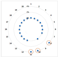 | 0.9 s | 14 s | 578 |
| Instance | Data Size | 1D1R | 1D2R | 2D1R | 2D2R | 3D1R | 3D2R | 4D1R | 4D2R | 5D1R | 5D2R |
|---|---|---|---|---|---|---|---|---|---|---|---|
| r50_5_1 | 50 | 205 | 179 | 193 | 177 | 177 | 177 | 184 | 187 | 180 | 177 |
| r50_5_2 | 50 | 209 | 185 | 204 | 182 | 201 | 184 | 184 | 199 | 184 | 184 |
| r50_5_3 | 50 | 190 | 188 | 188 | 190 | 190 | 188 | 188 | 188 | 190 | 188 |
| C101 | 100 | 2514 | 2513 | 2497 | 2498 | 2518 | 2494 | 2501 | 2477 | 2464 | 2403 |
| RC1_2 | 200 | 7284 | 7093 | 7268 | 7070 | 7280 | 7020 | 7322 | 7148 | 7116 | 6842 |
| RC_6 | 600 | 23,858 | 22,170 | 23,732 | 22,066 | 22,779 | 21,221 | 21,847 | 21,121 | 21,104 | 20,436 |
| R1_8 | 800 | 37,783 | 37,971 | 36,148 | 36,087 | 36,117 | 36,028 | 37,071 | 36,299 | 36,269 | 34,759 |
| R2_8 | 800 | 37,720 | 36,786 | 38,643 | 38,131 | 36,684 | 36,572 | 36,551 | 35,832 | 36,047 | 35,131 |
| C1_10 | 1000 | 44,856 | 46,461 | 41,718 | 43,429 | 44,029 | 41,369 | 44,130 | 44,810 | 41,711 | 41,131 |
| C2_10 | 1000 | 42,551 | 41,086 | 42,450 | 42,085 | 43,454 | 40,553 | 40,883 | 40,593 | 40,906 | 40,114 |
| Instance | MIP (5 h) | ALNS (1 min) | ALNS (2 min) | ALNS (5 min) | ALNS (10 min) | |||||
|---|---|---|---|---|---|---|---|---|---|---|
| Sol | BKB * Gap | Sol | BKS ** Gap | Sol | BKS Gap | Sol | BKS Gap | Sol | BKS Gap | |
| C1_10 | 37,811 | 72% | 39,268 | 4% | 37,751 | 0% | 36,287 | −4% | 35,624 | −6% |
| C2_10 | 39,753 | 54% | 41,483 | 4% | 38,968 | −2% | 36,912 | −7% | 35,648 | −10% |
| R1_10 | 54,370 | 47% | 47,738 | −12% | 47,017 | −14% | 45,731 | −16% | 44,526 | −18% |
| R2_10 | 52,413 | 45% | 48,730 | −7% | 47,272 | −10% | 45,443 | −13% | 44,340 | −15% |
| RC1_10 | 53,400 | 57% | 45,671 | −14% | 44,642 | −16% | 43,020 | −19% | 42,127 | −21% |
| Avg. | 47,549 | 55% | 44,578 | −5% | 43,130 | −8% | 41,478 | −12% | 40,453 | −14% |
| Instance | MIP 3 h | ALNS 30 s | ALNS 60 s | ALNS 90 s | ALNS 120 s | |||||
|---|---|---|---|---|---|---|---|---|---|---|
| Sol | BKB Gap | Sol | BKS Gap | Sol | BKS Gap | Sol | BKS Gap | Sol | BKS Gap | |
| C1_10 | 48,058 | 78% | 41,131 | −14% | 39,268 | −18% | 38,366 | −20% | 37,751 | −21% |
| C2_10 | 47,728 | 62% | 43,114 | −10% | 41,483 | −13% | 40,036 | −16% | 38,968 | −18% |
| R1_10 | 69,597 | 59% | 49,655 | −29% | 47,738 | −31% | 47,321 | −32% | 47,017 | −32% |
| R2_10 | 69,010 | 59% | 50,866 | −26% | 48,730 | −29% | 47,981 | −31% | 47,272 | −32% |
| RC1_10 | 55,882 | 59% | 47,048 | −16% | 45,671 | −18% | 44,702 | −20% | 44,642 | −20% |
| Avg. | 58,055 | 63% | 46,363 | −19% | 44,578 | −22% | 43,681 | −24% | 43,130 | −25% |
| Instance | MIP 3 h | ALNS 30 s | ALNS 60 s | ALNS 90 s | ALNS 120 s | |||||
|---|---|---|---|---|---|---|---|---|---|---|
| Sol | BKB Gap | Sol | BKS Gap | Sol | BKS Gap | Sol | BKS Gap | Sol | BKS Gap | |
| C1_8 | 43,489 | 81% | 27,893 | −36% | 27,279 | −37% | 26,891 | −38% | 26,646 | −39% |
| C2_8 | 40,022 | 63% | 30,549 | −24% | 29,330 | −27% | 28,770 | −28% | 28,422 | −29% |
| R1_8 | 49,105 | 59% | 35,861 | −27% | 34,752 | −29% | 33,983 | −31% | 33,490 | −32% |
| R2_8 | 43,725 | 54% | 35,131 | −20% | 34,763 | −20% | 34,042 | −22% | 33,722 | −23% |
| RC1_8 | 45,585 | 64% | 35,623 | −22% | 34,639 | −24% | 34,139 | −25% | 33,807 | −26% |
| Avg. | 44,385 | 64% | 33,012 | −26% | 32,153 | −28% | 31,565 | −29% | 31,217 | −30% |
| Instance | MIP 3 h | ALNS 30 s | ALNS 60 s | ALNS 90 s | ALNS 120 s | |||||
|---|---|---|---|---|---|---|---|---|---|---|
| Sol | BKB Gap | Sol | BKS Gap | Sol | BKS Gap | Sol | BKS Gap | Sol | BKS Gap | |
| C1_6 | 17,706 | 64% | 18,862 | 7% | 18,452 | 4% | 18,140 | 2% | 17,884 | 1% |
| C2_6 | 21,190 | 46% | 21,491 | 1% | 20,709 | −2% | 19,935 | −6% | 19,663 | −7% |
| R1_6 | 22,780 | 43% | 21,458 | −6% | 21,072 | −7% | 20,873 | −8% | 20,729 | −9% |
| R2_6 | 23,286 | 44% | 21,733 | −7% | 21,209 | −9% | 21,003 | −10% | 20,796 | −11% |
| RC1_6 | 20,978 | 49% | 20,325 | −3% | 19,871 | −5% | 19,618 | −6% | 19,392 | −8% |
| Avg. | 13,441 | 49% | 20,774 | −2% | 20,263 | −4% | 19,914 | −6% | 19,693 | −7% |
| Instance | MIP 3 h | ALNS 30 s | ALNS 60 s | ALNS 90 s | ALNS 120 s | |||||
|---|---|---|---|---|---|---|---|---|---|---|
| Sol | BKB Gap | Sol | BKS Gap | Sol | BKS Gap | Sol | BKS Gap | Sol | BKS Gap | |
| C1_4 | 12,518 | 69% | 12,662 | 1% | 12,518 | 0% | 12,283 | −2% | 12,133 | −3% |
| C2_4 | 12,523 | 51% | 12,697 | 1% | 12,343 | −1% | 12,252 | −2% | 12,218 | −2% |
| R1_4 | 14,414 | 45% | 14,424 | 0% | 13,877 | −4% | 13,579 | −6% | 13,524 | −6% |
| R2_4 | 14,490 | 49% | 14,638 | 1% | 14,105 | −3% | 13,985 | −3% | 13,916 | −4% |
| RC1_4 | 14,034 | 55% | 13,811 | −2% | 13,501 | −4% | 13,211 | −6% | 13,026 | −7% |
| Avg. | 13,596 | 54% | 13,646 | 0% | 13,269 | −2% | 13,062 | −4% | 12,963 | −5% |
| Instance | MIP 3 h | ALNS 30 s | 60 s | ALNS 90 s | ALNS 120 s | |||||
|---|---|---|---|---|---|---|---|---|---|---|
| Sol | BKB Gap | Sol | BKS Gap | Sol | BKS Gap | Sol | BKS Gap | Sol | BKS Gap | |
| C1_2 | 6757 | 70% | 6834 | 1% | 6679 | −1% | 6555 | −3% | 6489 | −4% |
| C2_2 | 6998 | 57% | 6734 | −4% | 6667 | −5% | 6626 | −5% | 6583 | −6% |
| R1_2 | 7735 | 55% | 7054 | −9% | 6973 | −10% | 6944 | −10% | 6917 | −11% |
| R2_2 | 7368 | 52% | 7112 | −3% | 6962 | −6% | 6911 | −6% | 6887 | −7% |
| RC1_2 | 6725 | 55% | 6779 | 1% | 6617 | −2% | 6593 | −2% | 6567 | −2% |
| Avg. | 7117 | 56% | 6903 | −3% | 6780 | −5% | 6726 | −5% | 6689 | −6% |
| Instance | MIP 3 h | ALNS 30 s | ALNS 60 s | ALNS 90 s | ALNS 120 s | |||||
|---|---|---|---|---|---|---|---|---|---|---|
| Sol | BKB Gap | Sol | BKS Gap | Sol | BKS Gap | Sol | BKS Gap | Sol | BKS Gap | |
| C101 | 2390 | 63% | 2403 | 1% | 2403 | 1% | 2389 | 0% | 2389 | 0% |
| C201 | 2615 | 55% | 2720 | 4% | 2717 | 4% | 2637 | 1% | 2636 | 1% |
| R101 | 2274 | 37% | 2284 | 0% | 2284 | 0% | 2245 | −1% | 2183 | −4% |
| R201 | 2192 | 37% | 2173 | −1% | 2165 | −1% | 2165 | −1% | 2106 | −4% |
| Rc101 | 2904 | 53% | 3054 | 5% | 3045 | 5% | 2907 | 0% | 2907 | 0% |
| Avg. | 2475 | 49% | 2527 | 2% | 2523 | 2% | 2469 | 0% | 2444 | −1% |
| Instance | MIP 3 h | ALNS 30 s | ALNS 60 s | ALNS 90 s | ALNS 120 s | |||||
|---|---|---|---|---|---|---|---|---|---|---|
| Sol | BKB Gap | Sol | BKS Gap | Sol | BKS Gap | Sol | BKS Gap | Sol | BKS Gap | |
| r50_5_1 | 168 | 28% | 177 | 5% | 177 | 5% | 177 | 5% | 177 | 5% |
| r50_5_2 | 139 | 30% | 185 | 33% | 184 | 32% | 184 | 32% | 184 | 32% |
| r50_5_3 | 150 | 31% | 188 | 25% | 188 | 25% | 188 | 25% | 188 | 25% |
| r50_5_4 | 196 | 34% | 194 | −1% | 184 | −6% | 184 | −6% | 183 | −7% |
| r50_5_5 | 184 | 33% | 185 | 1% | 185 | 1% | 174 | −5% | 174 | −5% |
| Avg. | 167 | 31% | 186 | 13% | 184 | 12% | 181 | 10% | 181 | 10% |
| Instance | MIP 0.5 h | ALNS 30 s | ALNS 60 s | ALNS 90 s | ALNS 120 s | |||||
|---|---|---|---|---|---|---|---|---|---|---|
| Sol | BKB Gap | Sol | BKS Gap | Sol | BKS Gap | Sol | BKS Gap | Sol | BKS Gap | |
| r50_5_1 | 180 | 29% | 177 | −2% | 177 | −2% | 177 | −2% | 177 | −2% |
| r50_5_2 | 185 | 31% | 185 | 0% | 184 | −1% | 184 | −1% | 184 | −1% |
| r50_5_3 | 188 | 34% | 188 | 0% | 188 | 0% | 188 | 0% | 188 | 0% |
| r50_5_4 | 187 | 36% | 194 | 4% | 184 | −2% | 184 | −2% | 183 | −2% |
| r50_5_5 | 197 | 37% | 185 | −6% | 185 | −6% | 174 | −12% | 174 | −12% |
| Avg. | 187 | 33% | 186 | −1% | 184 | −2% | 181 | −3% | 181 | −3% |
Disclaimer/Publisher’s Note: The statements, opinions and data contained in all publications are solely those of the individual author(s) and contributor(s) and not of MDPI and/or the editor(s). MDPI and/or the editor(s) disclaim responsibility for any injury to people or property resulting from any ideas, methods, instructions or products referred to in the content. |
© 2023 by the authors. Licensee MDPI, Basel, Switzerland. This article is an open access article distributed under the terms and conditions of the Creative Commons Attribution (CC BY) license (https://creativecommons.org/licenses/by/4.0/).
Share and Cite
Saker, A.; Eltawil, A.; Ali, I. Adaptive Large Neighborhood Search Metaheuristic for the Capacitated Vehicle Routing Problem with Parcel Lockers. Logistics 2023, 7, 72. https://doi.org/10.3390/logistics7040072
Saker A, Eltawil A, Ali I. Adaptive Large Neighborhood Search Metaheuristic for the Capacitated Vehicle Routing Problem with Parcel Lockers. Logistics. 2023; 7(4):72. https://doi.org/10.3390/logistics7040072
Chicago/Turabian StyleSaker, Amira, Amr Eltawil, and Islam Ali. 2023. "Adaptive Large Neighborhood Search Metaheuristic for the Capacitated Vehicle Routing Problem with Parcel Lockers" Logistics 7, no. 4: 72. https://doi.org/10.3390/logistics7040072
APA StyleSaker, A., Eltawil, A., & Ali, I. (2023). Adaptive Large Neighborhood Search Metaheuristic for the Capacitated Vehicle Routing Problem with Parcel Lockers. Logistics, 7(4), 72. https://doi.org/10.3390/logistics7040072