Optimization of the Residual Biomass Supply Chain: Process Characterization and Cost Analysis

Abstract

Background: This study investigates the vital significance of logistical cost optimization within the residual woody biomass supply chain, aiming to boost both sustainability and the efficient uti-lization of this resource. There is an emphasis on how adept cost management can determine the economic feasibility of exploiting residual biomass. Methods: The research delves into crucial areas including collection, transportation, storage, and processing of biomass, highlighting their re-spective roles in the total cost. The influence of factors such as seasonality and biomass quality variations on the supply chain's cost and efficiency is explored. To provide an in-depth analysis of these factors, mathematical models are presented that allow for the examination of a variety of scenarios and optimization strategies. Techniques such as linear programming, genetic algo-rithms, and tabu search are contextualized within these models. Results: The study provides in-sights into individual cost contributions of different logistical operations. It also reveals how seasonality and biomass quality variations directly affect the cost and efficacy of the supply chain. Conclusions: Proficient logistical cost management is crucial for the successful exploitation of re-sidual biomass. The findings have substantial implications for managing the residual biomass supply chain, paving the way for a transition to a low-carbon economy.

1. Introduction

The viability of any value chain based on residual biomass, which includes forestry and agricultural waste, is critically influenced by the logistical costs associated with its collection [1]. This potential raw material for renewable fuels, chemicals, and energy production is currently underutilized, with only 40% to 60% of the total collected volume being used, leading to significant resource wastage [2,3,4]. Despite the competitive cost of energy generation from biomass compared to fossil fuels, the logistical constraints related to biomass collection and transportation often render these processes unfeasible [5,6]. The supply system for this raw material involves numerous unit operations, such as collection, preprocessing, transportation, and storage, which present significant technical and logistical challenges [7,8]. These operations require a variety of transport equipment to move the biomass from its source to the conversion and valorization site [9,10].

The optimization of the supply chain for biomass energy valorization units is a crucial research area, given the increasing focus on renewable energy sources and the decarbonization of industrial production and mobility [11,12]. This optimization is a complex problem due to various supply and demand constraints [13]. The transportation costs of residual biomass constitute the majority of the supply chain costs for energy production, thus attracting attention from several recent studies on methodologies for optimizing logistical processes and reducing total operation costs [14,15]. The viability of biomass supply chains is heavily dependent on the optimization of these logistical processes, which include all operations from collection to delivery of the biomass at the processing site [16,17]. This involves considerations about the location of potential biomass storage parks, the location of processing units, the methods and equipment used for collection and transportation, and the ability to store and treat biomass to optimize its utilization [18]. Given the complexity of the processes and the large number of operations involved, optimizing logistical processes is a critical aspect of ensuring the economic viability of biomass supply chains [19].

Several previous studies addressed these complex subjects and contributed to the broader discussion on supply chain management, with a particular focus on the management of residual biomass and other resources. For example, Shahsavani and Goli and Lotfi et al. emphasized the importance of sustainable and efficient supply chain management [20,21]. Shahsavani and Goli focused on the concept of a circular supply chain, which aims to reduce total energy consumption. This aligns with the broader goal of managing residual biomass, which is to utilize waste resources efficiently and sustainably. Lotfi et al. proposed a robust, risk-aware, resilient, and sustainable closed-loop supply chain network design, which could be applied to the management of residual biomass. Del Rosario et al. provided an overview of sustainable development and the Sustainable Development Goals, which are relevant to the management of residual biomass as this contributes to several of the goals, including responsible consumption and production, and climate action [22]. Shokouhifar and Ranjbarimesan and Shokouhifar et al. both proposed models to improve supply chain management [23,24]. Shokouhifar and Ranjbarimesan focus on the blood supply chain, but their proposed model could potentially be applied to the management of residual biomass. Shokouhifar et al. proposed a multi-product and multi-objective model for managing the phosphorus fertilizer supply chain, which could also be relevant to the management of residual biomass. Salehi et al. and Nunes et al. focused specifically on the management of biomass [1,25]. Salehi et al. proposed a resilient and sustainable biomass supply network, which aligns closely with the goals of residual biomass management. Nunes et al. analyzed the supply chain associated with the energy recovery of agroforestry woody residual biomass, identifying the main constraints and potential solutions. However, each study approached the topic from a unique perspective, offering different insights and solutions.

The logistical process associated with the collection of residual biomass presents a complex challenge that is critical for promoting a circular and sustainable economy [26]. Efficient utilization of this energy source requires a well-managed and optimized supply chain, from collection, transportation, and storage to energy conversion [27,28]. The logistics associated with this supply chain are highly complex, involving multiple actors, pieces of equipment, and operations [29,30]. The dispersed and diffuse nature of the residual biomass collection sites contributes to high costs, making the minimization of transportation distance and efficient planning of collection routes critical elements in optimizing the logistic process [31,32]. Several optimization models and techniques, such as linear programming models, genetic algorithms (GA), and tabu search (TS), have been applied to this problem [33,34,35]. However, these models have limitations, particularly when dealing with the complexity and uncertainty inherent in the biomass supply chain [36]. To handle these complexities and uncertainties, more advanced optimization techniques have been developed [35]. While both GA and TS have demonstrated effectiveness in solving complex optimization problems, each has its own advantages and disadvantages [37]. The choice of optimization technique depends on the specific characteristics of the logistical problem in question. It is important to note that optimizing the logistical process associated with residual biomass collection is not just a matter of cost minimization. It also involves ensuring the sustainability and long-term viability of the biomass supply chain, which implies considering a range of factors such as biomass availability and quality, environmental conditions, legal and policy constraints, and the needs and preferences of stakeholders [38,39].

The main objective of this article is to delve into and thoroughly analyze the logistical process associated with the collection of residual biomass. The main contributions of this study are:

• Understanding the inherent complexities of the residual biomass supply chain and identifying efficient and sustainable optimization strategies.
• Emphasizing the use of optimization techniques, such as linear programming, genetic algorithms, and tabu search, and their potential to enhance the efficiency and sustainability of this logistical process.
• Applying these tools to minimize operational costs in an integrated manner.
• Examining the various constraints and challenges that may emerge in this context, such as biomass quality and availability, environmental conditions, legal and policy constraints, and stakeholder needs.
• Providing a comprehensive understanding of this subject, which can inform and guide future decisions and practices in the field of residual biomass collection and recovery.

2. Organization of the Work

This article is organized into five main sections, as follows:

• Section 1, the Introduction, provides an overview of the topic and sets the context for the subsequent discussions. It outlines the importance of understanding and optimizing the logistics of residual biomass collection, and the potential benefits that can be derived from such efforts. The introduction also highlights the research gap that this article aims to address.
• Section 2, Organization of the Work, outlines the structure of the article and provides a roadmap for the reader. It describes the sequence of topics that will be discussed and explains how each section contributes to the overall objective of the article.
• Section 3, Literature Review, presents analysis of previous works related to the subject of this research and outlines the contributions of this manuscript comparatively with the existing literature.
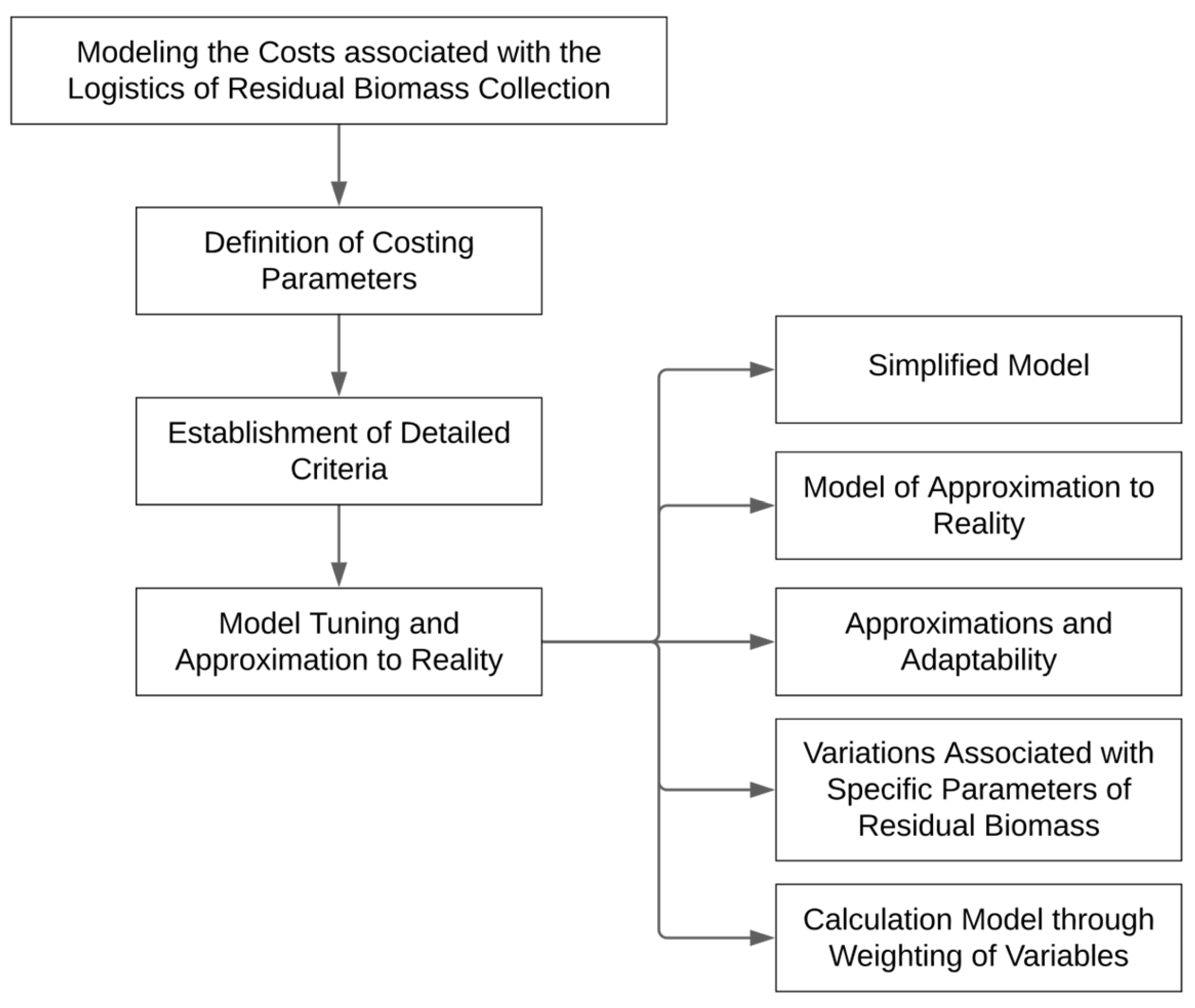
• Section 4, Modeling the Costs Associated with the Logistics of Residual Biomass Collection, is organized as presented in Figure 1. It begins with the Definition of Costing Parameters, where the various factors that contribute to the cost of logistics are identified and defined. This is followed by the Establishment of Detailed Criteria, where these parameters are further refined and categorized. The section then moves on to Model Tuning and Approximation to Reality, which is further divided into five subsections. The Simplified Model provides a basic understanding of the cost structure, while the Model of Approximation to Reality introduces more complexity and realism. The Approximations and Adaptability subsection discusses the flexibility of the model and its ability to adapt to different scenarios. The Variations Associated with Specific Parameters of Residual Biomass subsection examines how changes in the characteristics of the biomass can affect the costs. Finally, the Calculation Model through Weighting of Variables presents a method for quantifying the costs based on the defined parameters and criteria.
• Section 5, Optimization Models for the Collection Process, presents different models for optimizing the logistics of residual biomass collection. It starts with a Linear Approach for the Characterization of the Supply Chain, which provides a simplified model for understanding the logistics process. This is followed by Complex Models, which introduce more sophisticated methods for optimizing the collection process.
• Section 6, Conclusions, summarizes the key findings of the article. It highlights the implications of the cost models and optimization methods discussed in the previous sections and suggests directions for future research. This section also reiterates the importance of understanding and optimizing the logistics of residual biomass collection, and the potential benefits that can be derived from such efforts.

3. Literature Review

The exploration of the logistical process associated with the collection of residual biomass has been the focus of numerous studies in recent years. This interest can be attributed to the growing recognition of the potential of residual biomass as a sustainable energy source coupled with the challenges posed by its collection and utilization. This current study contributes to the existing knowledge by delving into the inherent complexities of the residual biomass supply chain. These complexities encompass a wide range of factors, from the physical characteristics of the biomass itself to the logistical challenges of collection, transportation, and storage. By providing a detailed analysis of these complexities, the study offers valuable insights that can help to inform more effective and efficient strategies for residual biomass collection. In addition to identifying these complexities, the study also proposes efficient and sustainable optimization strategies. These strategies are designed to address the identified complexities and enhance the overall efficiency and sustainability of the residual biomass supply chain. The proposed strategies include the use of advanced optimization techniques, such as linear programming, genetic algorithms, and tabu search, which have been shown to be effective in addressing similar challenges in other supply chain contexts.

The approach followed here aligns with the works of Atashbar et al. (2016), Sun and Fan (2020), Lo et al. (2021), and Ba et al. (2016), who also emphasized the need for a comprehensive understanding of the supply chain in their study of the residual biomass sector [19,40,41,42]. These previous works, among others, provided a valuable foundation by highlighting the importance of a holistic understanding of the supply chain, including the various stages of the process and the interactions between them. However, this study extends their work by not only identifying the complexities inherent in the residual biomass supply chain but also proposing specific, actionable strategies for optimization. This represents a significant advancement in the field, as it moves beyond a mere understanding of the challenges to the development of practical solutions that can be implemented in real-world contexts.

The application of optimization techniques, including linear programming, genetic algorithms, and tabu search, is a key contribution of this study, which is in line with previous studies such as Jauhar and Pant (2016), Min (2015), Sang (2021), and Radhakrishnan et al. (2009) [43,44,45,46]. However, this study underscores these techniques’ potential to augment both the efficiency and sustainability of the logistical process involved in residual biomass collection. Linear programming, a mathematical method used to find the best possible outcome in a given mathematical model, has been widely used in supply chain management to optimize various aspects such as cost, time, and resources [16,34,40,47]. Similarly, genetic algorithms (GA), inspired by the process of natural selection, have been used to solve optimization problems in biomass supply chain management, as can be demonstrated by the studies of Pinho et al. (2018), Castillo-Vilar (2014), De Meyer et al. (2014), and Sarker et al. (2019) [48,49,50,51]. This previous research demonstrated that these algorithms are useful in dealing with complex, multi-objective problems, as they can explore a large solution space and find near-optimal solutions. Another optimization technique, tabu search, has also been used in previous studies to solve specific problems in the biomass supply chain. For example, Cao et al. (2021), Edwards et al. (2015), and An et al. (2011) used this method, known for its ability to avoid local optima and explore the solution space more thoroughly [52,53,54]. In contrast to previous studies that have applied these techniques to specific aspects of the supply chain, the current study adopts a more holistic approach. It emphasizes the potential of these optimization techniques to enhance the efficiency and sustainability of the entire logistical process, from the collection of residual biomass to its final use. This novel approach provides a more comprehensive understanding of the potential of these techniques and sets a new direction for future research in this field. The same situation can be described with regards to the application of these tools to minimize operational costs in an integrated approach. While Sharma et al. (2013) and Durmaz and Bilgen (2020) also used optimization techniques to reduce costs, their approach was not integrated, focusing instead on individual components of the supply chain [55,56].

The examination of various constraints and challenges, such as biomass quality and availability, environmental conditions, legal and policy constraints, and stakeholder needs, is another area where this study contributes to the existing literature. Previous studies, such as those by Gallik et al. (2021), Wang et al. (2020), and Gómez-Marín and Bridgwater (2021), have discussed these constraints and challenges [57,58,59]. However, once again, the approach followed here examines these issues in the context of the entire logistical process, which can inform and guide future decisions and practices in the field of residual biomass collection.

4. Modeling the Costs Associated with the Logistics of Residual Biomass Collection

4.1. Definition of Costing Parameters

To develop a comprehensive mathematical model that effectively encompasses all stages of the process and the associated costs involved in the operations of cutting, cleaning, rechipping, loading, and transporting residual woody biomass to the final processing site, it is essential to take into consideration a series of factors [60]. These elements are not limited solely to variables directly involved in biomass handling but also incorporate contextual and environmental variables that can have a significant impact on the efficiency and economic viability of the process [61]. Among the various elements to be considered, intrinsic characteristics of the biomass such as type, density, and moisture stand out as they can influence both the difficulty of handling and the energy potential of the material [62]. Additionally, logistical factors such as distance and accessibility from the collection site to the processing location, the type of transport vehicle used, and its loading capacity are equally crucial for a proper analysis of the process and its operations [63]. Seasonality and climatic variation also play an important role, as they can affect biomass availability and transportation conditions [64]. Furthermore, economic factors such as labor and equipment costs, as well as the market value of biomass, must be incorporated into the model [65]. In addition, regulatory or policy restrictions that may limit biomass harvesting or impose specific quality standards should not be overlooked [66]. Finally, the uncertainty and variability associated with many of these variables must be considered, enabling the creation of a robust and resilient model capable of dealing with the complex and dynamic reality of biomass supply [67]. Thus, the challenge of modeling this process lies in striking a balance between accuracy and complexity, creating a model that is detailed enough to be precise yet simple enough to be practical and feasible for implementation.

Based on these assumptions, it is possible to identify a preliminary set of costs that can be considered primary and represent the main operations constituting the supply chain of residual or surplus woody biomass, which can originate from both forestry sources and agro-industrial production processes, as previously mentioned.

• Cutting cost (C_c): may include labor cost, equipment cost, and equipment maintenance cost, and can also be influenced by factors such as the type of biomass and site conditions.
• Cleaning cost (C_l): the cost associated with preparing the biomass for transportation. This may include debris removal, biomass separation from other materials, and the selection of distinct parts that constitute this biomass, such as the separation of husks.
• Recollection cost (C_r): the cost of collecting the biomass and preparing it for transportation, which may include biomass compaction (baling) and loading it onto transport vehicles or using more traditional methods (now making a comeback), such as modern animal traction.
• Loading cost (C_ca): the cost of loading the biomass onto the transport vehicle, which can vary depending on the type of vehicle used and the amount of biomass that needs to be loaded.
• Transportation cost (C_t): the cost of moving the biomass from the cutting site to the final processing site, which may include the cost of fuel, vehicle wear and tear, and time spent in transportation.

Therefore, a simple mathematical model to represent the total cost (C_T) of this process can be expressed as follows, referring to the sum of each of the identified components:

$$C_T=C_c+C_l+C_r+C_{ca}+C_t$$

(1)

4.2. Establishment of Detailed Criteria

The mathematical model introduced in the previous section represents a simplified version of reality, which, although useful for illustrating the fundamental dynamics of residual biomass collection, does not encompass all the cost factors that may arise in a real and practical situation. For example, the model does not account for the costs associated with biomass acquisition. These costs can vary depending on the origin of the biomass, the specifics of the acquisition contract, and potential transaction-related costs such as commissions, taxes, fees, or others. Additionally, costs related to waste management generated in the process must be considered. Depending on environmental regulations and waste management practices, the management of residual materials can entail significant costs when, for example, it requires contracting an entity to handle such waste. Another factor not considered in the simplified model is the cost of insurance policies. The operation of collecting and transporting biomass can involve significant risks and, therefore, adequate insurance coverage must be ensured. Insurance costs can vary depending on the nature of the operations, the type of selected insurance coverage, and other additional factors, depending on the complexity and scale of the process. Furthermore, obtaining the necessary licenses and permits to carry out biomass collection and transportation can be an expensive and time-consuming process. The simplified model does not take into account these costs, or the time required to obtain such licenses. Finally, there are several other indirect costs that may be associated with the process of residual biomass collection. These may include administrative costs, equipment maintenance costs, and personnel training costs, among others. Therefore, it is important to bear in mind that although the presented mathematical model is a useful tool for understanding the basic dynamics of residual biomass collection, it does not capture all the nuances and complexities that may be present in a real situation. For a more comprehensive and accurate analysis, it is necessary to develop a more comprehensive model that includes these and other potential cost factors. Thus, the mathematical model can be expanded to include additional parameters, such as:

• Biomass acquisition cost (C_a): the cost of acquiring biomass and may depend on a variety of factors, including the type of biomass and its location and spatial distribution.
• Waste management cost (C_d): the cost associated with managing any waste produced during the process of cutting, cleaning, reloading, loading, and transporting biomass.
• Insurance coverage cost (C_i): the cost of insuring the process, including equipment insurance and insurance for liability, environmental and work accidents, among others.
• Permit/license cost (C_p): the cost associated with obtaining the necessary permits and licenses to carry out the process.
• Indirect cost (C_in): a general cost that may include things such as administration, supervision, facility maintenance, and so on.

With these additional parameters, the mathematical model for the total cost (C_T) acquires a new formulation, which now includes all these additional parameters, thus making the model increasingly closer to reality.

$$C_T=C_c+C_l+C_r+C_{ca}+C_t+C_a+C_d+C_i+C_p+C_{in}$$

(2)

This is a more comprehensive model, but it is still simplified and may not encompass all possible cost variables. Furthermore, each of these costs can be a function of several other variables, and modeling these relationships can be complex. For instance, if there is an intermediate stop in the process where the material needs to be unloaded, processed, loaded again, and transported to the destination, these costs need to be added to the model:

• Unloading cost (C_de): the cost of unloading biomass at the intermediate location.
• Shredding cost (C_dt): the cost of shredding biomass at the intermediate location.
• Reloading cost (C_rc): the cost of reloading biomass onto the transport vehicle after shredding.
• Additional transportation cost (C_ta): the cost of transporting biomass from the intermediate location to the final processing location.

Thus, the mathematical model for the total cost (C_T) with an intermediate stop is:

$$C_T=C_c+C_l+C_r+C_{ca}+C_t+C_a+C_d+C_i+C_p+C_{in}+C_{de}+C_{dt}+C_{rc}+C_{ta}$$

(3)

However, this model remains a simplification. Once again, each of these costs can be a function of several other variables. For instance, the transportation cost (C_t and C_ta) could be subdivided into fuel cost, vehicle wear and tear, and transit time if these details were required for the analysis, and the same line of thinking can be applied to each of the other variables.

4.3. Model Tuning and Approximation to Reality

4.3.1. Simplified Model

The intricate relationships governing the management of residual biomass collection can be further explored at a deeper level by introducing a higher level of detail. This deepening of understanding of the process involves the inclusion of elements that may appear random at first glance but have a significant impact on the costs involved at each stage of the logistics process. For instance, meteorological variables such as precipitation and temperature can affect both the quality of biomass and the conditions for its collection. Additionally, factors such as fuel price fluctuations, changes in market conditions, or even alterations in legislation and regulations can influence costs and necessitate adjustments in logistics planning. By considering these variables, the management model must be sufficiently flexible to adapt to such fluctuations, thereby enabling continuous optimization of operations. This approach leads to a more realistic and precise assessment of the costs associated with residual biomass collection and facilitates more effective and efficient resource planning. This level of detail, although it may add complexity to the model, is crucial for effective management and truly efficient optimization of the residual biomass logistics chain. The level of detail can then be deepened in the following manner:

• Cutting cost (C_c): this cost can be influenced by factors such as labor cost (C_mo); labor productivity (P_mo), which may depend on workers’ education and experience; equipment cost (P_e), which may vary depending on the type and quality of the equipment; maintenance cost (M_e); equipment lifespan (L_e); and site conditions, which can affect cutting speed.

  $$C_c=\left(\frac{C_{mo}}{P_{mo}}\right)+\left(\frac{P_e}{L_e}\right)+C_{meq}$$

  (4)
• Cleaning cost (C_l): this cost can be influenced by factors similar to those of the cutting cost, such as labor productivity and equipment cost. It may also depend on the type of biomass and site conditions, among other factors.
• Reharvesting cost (C_r): this cost can be influenced by factors such as biomass size and shape, labor productivity, and equipment cost. For example, reharvesting larger biomass pieces may be more expensive than reharvesting smaller pieces, as it requires more effort from the equipment, resulting in increased fuel consumption.
• Loading cost (C_ca): this cost may depend on the type of vehicle used for transportation, the quantity of biomass that needs to be loaded, and labor productivity.
• Transportation cost (C_t): this cost may depend on factors such as the distance to the final processing location (D_pf), the type of vehicle used, fuel cost (C_comb), and the time required for travel (T_desl).

  $$C_t=\left(D_{pf}\times C_{comb}\right)+\left(T_{desl}\times C_{mo}\right)+\left(\frac{P_e}{L_e}\right)+M_e$$

  (5)

4.3.2. Model of Approximation to Reality

As previously mentioned, the situation will always be unique and may require the modification of these relationships to adapt to the specific conditions of a particular situation or location. However, the more detailed the model, the more accurate the calculation will be, allowing it to represent reality in a much closer manner. In other words, with the introduction of greater detail, the margin of error significantly decreases, although it still depends on the quality of the data used in the modeling. This level of detail can be presented as follows:

• Cutting cost (C_c): this cost can be represented as the sum of labor cost, equipment cost, and equipment maintenance cost. It can be assumed that the labor cost depends on the hourly rate (H) and the time required to cut the biomass (T_c). The equipment cost can be the price of the equipment (P_e) divided by its useful life (L_e), and the equipment maintenance cost (M_e) can be considered as a percentage of the equipment cost. Therefore, the formula can be presented as follows:

  $$C_c=H\times T_c+\left(\frac{P_e}{L_e}\right)+M_e$$

  (6)
• Cleaning cost (C_l): this cost can be represented similarly to the cutting cost, assuming that the time required for cleaning is T_l and the cleaning equipment has its own acquisition value (P_l), lifespan (L_l), and maintenance cost (M_l), as presented in the following equation:

  $$C_l=H\times T_l+\left(\frac{P_l}{L_l}\right)+M_l$$

  (7)
• Reharvesting cost (C_r): this cost can be influenced by the dimension and shape of the available biomass (S_b) if the amount of time required for recharging varies depending on the size of the pieces to be collected and processed. The recharging equipment has its own acquisition cost (P_r), useful life (L_r), and maintenance cost (M_r):

  $$C_r=H\times S_b\times T_r+\left(\frac{P_r}{L_r}\right)+M_r$$

  (8)
• Loading cost (C_ca): this cost can be influenced by the biomass quantity (Q_b) available if the time required for loading increases with the biomass quantity. The loading equipment also has its own acquisition value (P_ca), useful life (L_ca), and maintenance cost (M_ca).

  $$C_{ca}=H\times Q_b\times T_{ca}+\left(\frac{P_{ca}}{L_{ca}}\right)+M_{ca}$$

  (9)
• Transportation cost (C_t): this cost may depend on the distance to the final processing location (D), the fuel cost per kilometer (F), and the transit time (T_t). The vehicle has its own acquisition cost (P_v), useful life (L_v), and maintenance cost (M_v):

  $$C_t=D\times F+H\times T_t+\left(\frac{P_v}{L_v}\right)+M_v$$

  (10)

4.3.3. Approximations and Adaptability

Each analyzed situation will always be, or will be at least in the majority of cases, unique, with its own specificities, and may require the modification of these models to adapt to the intrinsic conditions of the ongoing operation. For example, labor productivity and equipment efficiency may vary, which would affect the time required for each task (T_c, T_l, T_r, T_ca, T_t). Furthermore, the cost of fuel may vary depending on factors such as equipment efficiency and fuel prices, which can change over time and may be dependent on external, uncontrollable factors. The quantity, size, and shape of biomass (S_b, Q_b) can also influence the time required to complete operations such as forwarding and loading. Therefore, it is important to keep in mind that these models are merely a starting point and may need to be adapted to fit specific situations.

From this perspective, when evaluating the cost calculation equation, it is easy to understand that each component has a complex relationship with the others. Each term in this formula not only represents an isolated cost but can also be influenced by other parameters. For this reason, the total cost is a function of these interconnected terms, where each one contributes to the optimization of the residual biomass supply chain. By understanding these relationships, it is possible to define a more accurate strategy for the most effective optimization, enabling more efficient resource management and maximizing return on investment. In this way, the approximation to reality of each of the relationships that exist for each of the terms described in the previously presented model can be presented.

$$C_T=C_c+C_l+C_r+C_{ca}+C_t+C_a+C_d+C_i+C_p+C_{in}$$

(11)

• Biomass acquisition cost (C_a): this cost may depend on the price per unit of biomass (P_b) and the quantity of biomass acquired (Q_b).

  $$C_a=P_b\times Q_b$$

  (12)
• Cost associated with waste management (C_d): this cost may depend on the quantity of waste produced (Q_r), which can be a proportion of the acquired biomass quantity and the cost per unit of waste to be managed (P_r):

  $$C_d=Q_r\times P_r$$

  (13)
• Insurance cost (C_i): this cost can correspond to a fixed rate or may depend on the value of the insured assets (V_a) and the insurance rate (I):

  $$C_i=V_a\times I$$

  (14)
• Cost associated with obtaining permits/licenses (C_p): this cost may depend on the number of permits or licenses required (N_p) and the cost per permit or license (P_p):

  $$C_p=N_p\times P_p$$

  (15)
• Indirect costs (C_in): this is a general cost that may include items such as administration, supervision, and facility maintenance. It can be difficult to model mathematically, but it can be considered as a percentage (α) of the total direct cost (C_direct), which is the sum of cutting, cleaning, reloading, loading, and transportation costs.

  $$C_{in}=\alpha \times C_{direto} \mathrm{where} C_{direto}=C_c+C_l+C_r+C_{ca}+C_t$$

  (16)

In the specific context described above, which includes an intermediate stop requiring the execution of multiple tasks, it is necessary to consider additional variables for calculating the corresponding costs. These variables are crucial in determining the costs of operations performed at this intermediate stop. Therefore, the cost model for this stage is defined by taking into account a series of components related to the operations carried out at this specific point in the logistics chain. Thus, given that this model is initially defined by the following equation, it is possible to establish a set of additional relationships:

$$C_T=C_c+C_l+C_r+C_{ca}+C_t+C_a+C_d+C_i+C_p+C_{in}+C_{de}+C_{dt}+C_{rc}+C_{ta}$$

(17)

• Unloading cost (C_de): this cost may depend on the quantity of biomass to be unloaded (Q_de), the time required for unloading (T_de), and the labor cost (H). Additionally, there may be an equipment cost associated with unloading.

  $$C_{de}=H\times Q_{de}\times T_{de}+\left(\frac{P_{de}}{L_{de}}\right)+M_{de}$$

  (18)
• Shredding cost (C_dt): this cost may depend on the dimensions and shape of the biomass (S_dt), the time required for shredding (T_dt), and the labor cost (H). Additionally, there may be an equipment cost associated with shredding.

  $$C_{dt}=H\times S_{dt}\times T_{dt}+\left(\frac{P_{dt}}{L_{dt}}\right)+M_{dt}$$

  (19)
• Reharvesting cost (C_rc): this cost may be similar to the loading cost, but it may depend on the quantity (volume) of biomass after shredding (Q_rc), the time required for recharging (T_rc), and the labor cost (H). Additionally, there may be equipment costs associated with recharging.

  $$C_{rc}=H\times Q_{rc}\times T_{rc}+\left(\frac{P_{rc}}{L_{rc}}\right)+M_{rc}$$

  (20)
• Additional transportation cost (C_ta): this cost may depend on the additional distance to the final processing location (D_a), the cost of fuel per kilometer (F), and the time for the additional displacement (T_ta). The vehicle has its own acquisition cost (P_v), useful life (L_v), and maintenance cost (M_v).

  $$C_{ta}=D_a\times F+H\times T_{ta}+\left(\frac{P_v}{L_v}\right)+M_v$$

  (21)

It is important to emphasize that optimizing supply chain costs is not merely a matter of minimizing individual costs. The objective should be to achieve the ideal balance among all the costs involved to maximize overall efficiency and operational profitability. Therefore, when evaluating the cost calculation model, it is crucial to understand the role that each component plays in the overall operations and how it relates to the other elements of the model.

4.3.4. Variations Associated with Specific Parameters of Residual Biomass

Let us assume that the biomass price (P_b) varies throughout the year according to a sinusoidal function, where P_max is the maximum price, P_min is the minimum price, and t is the time in months. The sinusoidal function has the property of reaching its maximum value in the middle of the period and its minimum value at the extremes of the period. Therefore, to model a higher price in winter (for example, if winter peaks in January, or t = 0) and a lower price in summer (for example, reaching the minimum in July, or t = 6), the cosine function can be used as follows:

$$P_{b\left(t\right)}=\left(\frac{P_{max}-P_{min}}{2}\right)\times \cos \left(2\times \pi \times \frac{t}{12}\right)+\left(\frac{P_{max}+P_{min}}{2}\right)$$

(22)

This equation assumes that the price variation is symmetric around the average of the maximum and minimum prices, and that the price variation follows a regular pattern throughout the year. However, in reality the price variation may not be perfectly symmetric or regular, and other factors beyond seasonality may affect the price of biomass. Therefore, this model is a simplification. It is based on the terms of a “standard year”, where t represents the month of the year ranging from 0 (January) to 11 (December). If one wishes to express t in terms of a specific year, it would be necessary to adjust the formula accordingly to the situation. This model can be incorporated into the biomass acquisition cost formula mentioned earlier by replacing P_b with P_b(t).

$$C_a\left(t\right)=P_b\left(t\right)\times Q_b$$

(23)

Since biomass is not a homogeneous resource, different types of biomass may have distinct characteristics that affect their value and usefulness. For example, moisture (H), the percentage of inert materials (I), and spatial dispersion (D) are factors that can significantly impact the value of different types of biomass. Therefore, it is reasonable to assume that different types of biomass may have different prices. In this context, the challenge is to develop and implement a logistical optimization model that can take these variables into account and provide an efficient and economically viable solution for the collection of residual biomass. Thus, the modeling, considering the effect of these factors to adjust the base price of biomass (P_b) with corresponding depreciation factors, could be defined as follows:

• Moisture: biomass with high moisture content may be less valuable because moisture reduces its calorific value and increases transportation costs (as the water is also being transported). Therefore, a depreciation factor for moisture (d_H) can be introduced, which decreases the price of biomass as moisture content increases.
• Inert percentage: biomass with a high percentage of inert materials may be less valuable because inert materials do not contribute to the energy value and can even cause damage to processing equipment, in addition to significantly contributing to the amount of ash produced if thermochemical conversion is the valorization pathway. Therefore, a depreciation factor for inert materials (d_I) can be introduced, which decreases the price of biomass as the percentage of inert materials increases.
• Spatial dispersion: biomass that is more scattered may be less valuable because it becomes more expensive to collect and transport. Therefore, a depreciation factor for spatial dispersion (d_D) can be introduced, which decreases the price of biomass as spatial dispersion increases.

Therefore, the adjusted biomass price ($P_b^{\prime }$) could be calculated as follows:

$$P_b^{\prime }=P_b\times \left(1-d_H\times H\right)\times \left(1-d_I\times I\right)\times \left(1-d_D\times D\right)$$

(24)

Next, P_b can be replaced with $P_b^{\prime }$ in the biomass acquisition cost formula.

$$C_a=P_b^{\prime }\times Q_b$$

(25)

However, it is necessary to take into consideration that the depreciation factors (d_H, d_I, d_D) are parameters that would need to be estimated based on historical data (preferably) or relevant literature. Furthermore, this is a simplification and the actual effect of these factors on biomass price may be more complex and nonlinear. For instance, the relationship between moisture and biomass price may vary across different moisture ranges. Therefore, it may be necessary to establish a more complex model to accurately capture these effects. In other words, it can be considered that the relationship between moisture and biomass price is not linear, but rather dependent on certain moisture thresholds. Hence, biomass moisture may not have a significant impact on price until it reaches a certain limit (H₁), after which the price starts to decrease. Furthermore, after a second threshold (H₂), the price decrease may be even more pronounced. This situation can be modeled using a piecewise function, where each “part” of the function has a different slope. For example:

• If H ≤ H₁, then d_H = 0 (there is no depreciation).
• If H₁< H ≤ H₂, then $d_H=a\times \left(H-H_1\right)$ (linear depreciation with slope a).
• If H > H₂, then $d_H=b\times \left(H-H_2\right)+a\times \left(H_2-H_1\right)$ (linear depreciation with slope b and a displacement to ensure the function is continuous).

Here, a and b are parameters representing the rate of price depreciation with respect to the humidity increase in different humidity intervals. H₁ and H₂ are the humidity thresholds. Therefore, the adjusted price of biomass ($P_b^{\prime }$) could be calculated as follows:

$$P_b^{\prime }=P_b\times \left(1-d_H\right)\times \left(1-d_I\times I\right)\times \left(1-d_D\times D\right)$$

(26)

Moreover, the acquisition cost of biomass would be:

$$C_a=P_b^{\prime }\times Q_b$$

(27)

This model assumes that the effects of humidity depreciation, percentage of inert materials, and spatial dispersion are independent and multiplicative, which may not be in reality entirely true. Additionally, this model assumes that depreciation is linear within each humidity interval, which may also not be true. Therefore, once again, this is a simplified model, and a more precise modeling of these effects may require additional data and more advanced modeling techniques. However, it is a tool that can be useful, if used judiciously, particularly for quick price assessments based on significant variations in the quality of materials to be acquired.

Table 1. Hypothetical data illustrating the variation of depreciation as a function of humidity.

% Humidity (H)	Depreciation Rate (dH)
0	0.00
10	0.00
20	0.05
30	0.10
40	0.15
50	0.25
60	0.35
70	0.45
80	0.55
90	0.65
100	1.00

presents an example of the definition of depreciation intervals, using humidity as an illustration.

In this example, it is assumed that there is no depreciation until the humidity reaches 20% (H₁ = 20). Between 20% and 50% humidity, the depreciation rate increases linearly from 0.00 to 0.15 (a = 0.15/30 = 0.005 per unit of humidity). Above 50% humidity (H₂ = 50), the depreciation rate increases more rapidly, from 0.15 to 0.65 (b = 0.50/50 = 0.01 per unit of humidity). This table can be used to construct a graph that shows the depreciation rate as a function of humidity. On the x-axis the humidity is plotted, and on the y-axis the depreciation rate is plotted. The graph would be a line that starts at 0.00, remains at 0.00 until H₁ = 20, then increases linearly to 0.15 at H₂ = 50, and then increases more rapidly to 1.00 at H = 100.

4.3.5. Calculation Model through Weighting of Variables

The use of historical data to calculate weighting factors in modeling the costs of a residual woody biomass supply chain offers several advantages. This approach allows for a more accurate estimation of costs as it is based on real observations, thereby improving the representativeness and relevance of the results. For example, incorporating historical data in determining operational costs such as cutting, cleaning, recharging, and transportation allows for the incorporation of the historical variability of these factors in the modeling process. This makes cost estimation more robust, reducing the risk associated with uncertainty. Furthermore, the inclusion of historical data allows for the consideration of temporal trends that may impact the supply chain, such as fluctuations in fuel prices or changes in labor productivity. By taking these trends into account, the company can better predict future needs and make informed strategic decisions. Therefore, starting with the following set of variables, which have been described in the previous sections, a model can be created where each variable is weighted according to its contribution to the total cost of the biomass acquisition process, including all logistical operations and potentially varying in detail depending on the context and utilization for these biomasses: cutting cost (C_c); cleaning cost (C_l); reharvesting cost (C_r); loading cost (C_ca); transportation cost (C_t); acquisition cost (C_a); unloading cost (C_d); chipping cost (C_i); post-chipping loading cost (C_p); intermediate transportation cost (C_in); unloading cost at the final destination (C_de); transportation cost to the final destination (C_dt); collection cost (C_rc); and transportation cost to storage (C_ta). Under this assumption, a series of weights (w₁, w₂, …, w₁₄) can be defined to reflect the relative importance of each of these specific costs in the total cost. For example, if the transportation cost is considered twice as important as the other costs, w₅ can be defined as 2 and all other weights as 1. The weighted total cost of biomass ($C_T^{\prime }$) could then be calculated as follows:

$$\begin{array}{c}{C}_T^{\prime }=w_1\times C_c+w_2\times C_l+w_3\times C_r+w_4\times C_{ca}+w_5\times C_t+w_6\times C_a+w_7\times C_d+w_8\times C_i+w_9\times C_p\hfill \\ \hspace{1em}\hspace{1em}\hspace{1em}\hspace{1em}\hspace{1em}\hspace{1em}\hspace{0.17em}+w_{10}\times C_{in}+w_{11}\times C_{de}+w_{12}\times C_{dt}+w_{13}\times C_{rc}+w_{14}\times C_{ta}\hfill \end{array}$$

(28)

The choice of weights used is highly dependent on the specific context. For example, in a situation where transportation is expensive and biomass resources are widely dispersed, the cost of transportation could be much more important than in a situation where biomass resources are located near the processing site. Similarly, if the biomass requires a significant amount of processing (e.g., if it contains a large amount of inert materials), the cost of cleaning and shredding could be more important. Therefore, the weights should be carefully chosen based on an understanding of the specific biomass supply system being modeled.

The assessment of the margin of error of a cost analysis model is essential to ensure the reliability of the predictions. By establishing this margin, one can grasp the variability and inherent uncertainty in the modeling, thus enabling a more accurate interpretation of the results. This procedure helps to avoid surprises or failures in planning, as it can guide strategic decision-making. Quantifying the margin of error allows for the identification of model limitations, encouraging continuous improvement and enhancement in cost forecasting, and contributing to the financial sustainability of the operation. The margin of error is a measure of the uncertainty associated with the estimates made by the model and can originate from various sources, including:

• Measurement errors: if the data used to calculate individual costs (C_c, C_l, …) are measurements, they may contain measurement errors.
• Parameter variation: the model parameters (e.g., weights w₁, w₂, …) can vary over time and/or space, or across different biomass supply systems.
• Cost variation: individual costs (C_c, C_l, …) can vary over time and/or space, or across different biomass supply systems.
• Model simplifications: the model may incorporate various simplifications (e.g., assuming costs are additive and that the effects of different variables are independent). These simplifications may not be exact, leading to errors in the estimation of total cost.

There are several ways to calculate the margin of error, depending on the sources of error that one wishes to consider.

• Error propagation: if there is an estimation of the error associated with each individual cost (e.g., due to measurement errors), one can utilize the theory of error propagation to calculate the margin of error in the total cost.
• Sensitivity analysis: if there is an understanding of how the model parameters (the weights w₁, w₂, …) can vary, a sensitivity analysis can be conducted to observe how the variation in these parameters affects the total cost.
• Simulation: if there is a probabilistic model of the biomass supply system (e.g., if the variation in costs and parameters has been modeled as random variables), simulation techniques such as the Monte Carlo method can be used to estimate the margin of error.

The assignment of weights (w₁, w₂, …, w₁₄) to the variables of the model is a process that fundamentally depends on a profound understanding of the system under analysis. This entails the utilization of relevant practical experience and consultation with experts in the field. Additionally, in specific situations, economic and statistical analyses can be employed to substantiate the selection of weighting factors. These methods help ensure that the weights adequately reflect the relative importance of each variable, thereby enhancing the accuracy and applicability of the model. This can involve the utilization of the following methodologies:

• Experience and industry knowledge: weights can be determined based on practical experience and industry knowledge. For example, if it is known that transportation costs are significantly higher than other operational costs, a higher weight can be assigned to transportation costs.
• Expert consultation: experts familiar with biomass production and transportation can be consulted. They can provide valuable insights into which costs are generally more significant.
• Economic analysis: an economic analysis can be conducted to determine the relative importance of each cost. For instance, evaluating how changes in each cost affect the total production cost or operational profitability.
• Sensitivity analysis: sensitivity analysis can be used to determine the impact of changes in each variable on the total cost. Variables that have the greatest impact on the total cost when changed can be assigned higher weights.
• Historical data analysis: if historical data on biomass production and transportation costs are available, statistical analyses can be used to determine which costs have had the greatest impact on the total cost over time.
• Optimization: in some cases, weights can be determined using optimization techniques. For example, defining an objective function (such as minimizing total cost or maximizing profit) and using optimization techniques to find the weights that optimize that function.

5. Optimization Models for the Collection Process

5.1. Linear Approach for the Characterization of the Supply Chain

Operations Research is a discipline that utilizes mathematical methods to make optimized decisions regarding complex problems. In optimizing the logistical process of residual biomass collection, a linear programming (LP) model can be particularly useful. Linear programming is a mathematical technique that enables the optimization (maximization or minimization) of a linear function subject to linear constraints. In the context of residual biomass logistics, the objective function could be the minimization of total collection and transportation costs of biomass, while the constraints could include the capacity of transportation vehicles, the availability of biomass at different locations, and the demand for processing sites, among others. LP is especially suitable for this type of problem for several reasons:

• Flexibility: LP allows for the inclusion of a variety of operational constraints, such as capacity limits, demand requirements, and time constraints.
• Computational efficiency: there already exist efficient algorithms (such as the simplex method) for solving LP problems.
• Interpretability: the solutions to an LP problem are easy to interpret. The optimal solution indicates the collection and transportation strategy that minimizes total costs, and the shadow prices (or reduced marginal costs) associated with constraints provide information about the method of minimizing those constraints.
• Sensitivity and scenario analysis: LP allows for sensitivity analysis to understand the impact of changes in model parameters (e.g., transportation costs, biomass availability) on the optimized solution. It also enables scenario analysis to explore alternative strategies under different assumptions or future conditions.

However, it is important to note that linear programming is based on certain assumptions (e.g., proportionality, additivity, divisibility, certainty) that may not hold true in all contexts of residual biomass logistics. If these assumptions are violated, other optimization techniques, such as integer programming, nonlinear programming, or stochastic programming, may be utilized. The choice of the optimization model depends, therefore, on the specific characteristics of the logistic problem at hand. As an example, consider a scenario characterized by the following assumptions, which includes multiple biomass collection locations and a single processing facility. Thus, i represents the set of all biomass collection locations (i = 1, 2, …, n); c_i is the cost of collection and transportation per unit of biomass at location i; q_i is the quantity of biomass available at location i; x_i is the amount of biomass to be collected at location i (decision variables); and Q is the required amount of biomass at the processing facility. Then, the objective function to be minimized (minimizing the total cost of collection and transportation) would minimize $\Sigma c_i\times x_i$ for all i, subject to a specific set of constraints:

• The amount of biomass collected at each location must not exceed the available quantity $x_i\le q_i$ (for all i).
• The total amount of biomass collected must meet the processing facility’s (demand) needs ($\Sigma x_i\ge Q$ for all i).
• The biomass quantities to be collected cannot be negative ($x_i\ge 0$ for all i).

This model can be expanded or modified to accommodate more complex features of the problem, such as multiple processing locations, limited transportation capabilities, and time-varying costs, among others. However, these modifications may result in an integer linear programming problem or a mixed integer linear programming problem, depending on the degree of complexity added. For instance, what if we want to add a constraint stating that the transportation vehicle cannot pick up less than half of its carrying capacity at each collection point? The inclusion of this new constraint implies that the amount collected at each point (x_i) must be greater than or equal to half of the vehicle’s carrying capacity. In other words, for a given vehicle carrying capacity (C), the constraint would be $x_i\ge 0.5\times C$, and the mathematical model would minimize $Z=\Sigma \left(c_i\times x_i\right)$ for all i, subject to:

• $\Sigma \left(x_i\right)$ for all $i\ge D$, where D is the search at the processing location;
• $x_i\le q_i$ for all i, where q_i is the quantity available at location i;
• $x_i\ge 0.5\times C$ for all i, where C is the vehicle’s carrying capacity;
• $x_i\ge 0$ for all i, ensuring that the collected quantity cannot be negative.

This constraint can make the problem more complex and potentially unsolvable if the vehicle’s carrying capacity is greater than the available quantity at some locations. In this situation, either the vehicle’s capacity or the collection strategy would need to be reassessed, for example, by introducing a new rule stating that the first load of the vehicle must comply with this constraint, while the second load does not, only requiring it to fill the entire truck’s capacity from the second load onwards. This condition certainly makes the problem more flexible and capable of being solved. To incorporate this condition into the model, it is necessary to introduce an additional binary variable that represents whether the vehicle is in its first load (y) or in the second load (1 − y). Therefore, the constraint would be modified to apply only to the first load. The mathematical model would then minimize $Z=\Sigma \left(c_i\times x_i\right)$ for all i, with:

• $\Sigma \left(x_i\right)$ for all $i\ge D$, where D is the demand at the processing location;
• $x_i\le q_i$ for all i, where q_i is the quantity available at location i;
• $x_i\ge 0.5\times C\times y$ for all i, where C is the vehicle’s carrying capacity and y is a binary variable (0 or 1);
• $x_i\ge 0$ for all i, ensuring that the collected quantity cannot be negative;
• y is a binary variable.

Thus, when y = 1 (indicating the first load), the constraint that the collected quantity must be at least half of the carrying capacity is applied. When y = 0 (indicating the second load), this constraint does not apply. However, this model assumes that the order of the loads is known in advance and can be fixed. Otherwise, the solution to the problem may become more complex and may require a more advanced optimization algorithm. For example, a genetic algorithm or a tabu search algorithm could be used to solve a vehicle routing problem with more complex capacity constraints.

As an application example, let us consider a scenario where there are three biomass collection sites and one processing facility. The costs of collection and transportation per unit of biomass at the three locations are 5€, 7€, and 4€, respectively. The quantities of biomass available at the three locations are 100, 200, and 150 units, respectively. The processing facility requires 300 units of biomass. The linear programming model for this problem can then be formulated as minimizing Z = 5x₁ + 7x₂ + 4x₃, subject to the conditions x₁ ≤ 100, x₂ ≤ 200, x₃ ≤ 150, x₁ + x₂ + x₃ ≥ 300, and x₁, x₂, x₃ ≥ 0. Solving this linear programming problem will give the optimal amounts of biomass to be collected at each location (x₁, x₂, x₃) that will minimize the total cost of collection and transportation. Now, let us assume that the problem is solved and it was found that the optimal solution is x₁ = 100, x₂ = 200, x₃ = 0. This means that all available biomass should be collected at the first two locations and none at the third location. The total cost of collection and transportation will be $5€\times 100+7€\times 200+4€\times 0=1900€$. This result provides valuable insights for decision-making. For example, it suggests that the third location, despite having a lower cost per unit of biomass, is not included in the optimal solution due to its lower availability of biomass compared to the other locations. This highlights the importance of considering both cost and availability in the decision-making process. However, it is important to note that this is a simplified example, and the actual problem may be more complex. For instance, there may be constraints on the capacity of transportation vehicles, time-varying costs, multiple processing locations, and other factors that need to be considered. In such cases, more advanced optimization techniques may be required.

5.2. Complex Models

A genetic algorithm (GA) is a technique that proves to be particularly effective in solving complex optimization problems. Its mode of operation is based on generating a set of candidate solutions, referred to as a population, which evolves iteratively through the application of operations analogous to natural selection, crossover, and mutation, which occur in nature. The GA is especially appreciated for its ability to efficiently explore many solutions when dealing with challenging or even impossible problems to solve using exact methods due to their computational complexity. These algorithms have been successfully applied in a variety of areas, from engineering and computer science to economics and logistics. The GA can be adjusted to adapt to the specificities of different problems, which gives it great flexibility. However, this characteristic also imposes the need for careful calibration of the algorithm’s parameters to ensure optimal performance. Through the successive generation of solutions, where each generation is a new “population” of routes, the genetic algorithm progressively refines the solutions, converging over time towards a route that, although not necessarily the globally optimal one, will be a high-quality solution to the problem. It is important to note that GAs are inherently heuristic. This means that they seek viable and efficient solutions to complex problems, but do not guarantee that the solution found will be the global optimum. This characteristic, which can be seen as a limitation, is a consequence of the pragmatic approach that GAs adopt to solve large-scale optimization problems, such as biomass collection logistics. Thus, although they do not guarantee the global optimal solution, genetic algorithms can offer highly efficient and viable solutions that can be successfully implemented in practice.

As an application example, let us consider a hypothetical scenario where there are five biomass collection sites (A, B, C, D, E) and we need to determine the optimal route for a collection vehicle to take to visit all sites and then return to the starting point. The distances between the sites are as follows (in km), as presented in

Table 2. Distances between the biomass collection sites (in km).

	A	B	C	D	E
A	0	10	15	20	25
B	10	0	5	15	20
C	15	5	0	10	15
D	20	15	10	0	5
E	25	20	15	5	0

.

Thus, the GA can be applied to solve the problem. The GA starts by generating a set of random routes (the initial population), for example, A-B-C-D-E-A, A-C-B-E-D-A, A-D-E-B-C-A, A-E-D-C-B-A, A-C-E-B-D-A, and so on. Each route is a candidate solution to the problem. The GA then evaluates each route based on a fitness function, which in this case is the total distance of the route. The shorter the distance, the better the solution. The GA then creates a new population by selecting the best routes (selection), combining them (crossover), and introducing small random changes (mutation). This process is repeated for a number of iterations, or until a satisfactory solution is found. After running the GA, for instance, for 100 iterations, the optimal route A-C-B-E-D-A, with a total distance of 45 km, is identified. This result shows that the GA was able to find a high-quality solution to the problem. Although it cannot be guaranteed that this is the absolute best solution (since GAs are heuristic and do not guarantee finding the global optimum), this is a highly efficient and viable solution that can be implemented in practice. By iteratively generating and refining solutions, GAs can efficiently explore a large solution space and find high-quality solutions.

Another potentially promising approach to the inherent challenge of managing the logistics of the biomass supply chain is the implementation of tabu search (TS), a metaheuristic optimization technique that is primarily known for its ability to overcome the common problem of local optima, which occurs when an algorithm gets stuck in a suboptimal solution, believing it has reached the best possible solution. The strength of TS lies in its “tabu list”, a dynamic record of the most recently explored solutions, which expressly prohibits revisiting those solutions for a certain number of iterations. This prohibition, which may seem counterintuitive, is actually what gives TS its effectiveness. By forcing the algorithm to explore new regions of the solution space instead of getting fixated on already-explored areas, TS allows for the discovery of truly optimal solutions that could otherwise go unnoticed. In this way, TS offers a robust and sophisticated approach to logistics optimization in the management of the biomass supply chain.

As an application example, let us consider a scenario with a biomass supply chain composed of five collection sites (A, B, C, D, E) and one processing site (P). The goal is to find the optimal route for collecting biomass from these sites and delivering it to the processing site. The distances between the sites and the processing site are, respectively, 10, 15, 20, 25, and 30 km. To find the optimal route, the algorithm starts with a random route, for instance, A-B-C-D-E-P. It then generates all possible neighboring routes by swapping two sites. For example, one neighboring route could be B-A-C-D-E-P (by swapping A and B). The algorithm evaluates the total distance of each neighboring route and selects the one with the shortest distance as the new current route. However, the swapped sites (A and B in this case) are added to the tabu list, which means that they cannot be swapped again for a certain number of iterations. The algorithm continues to generate neighboring routes, evaluate their total distances, and select the shortest one as the new current route, while updating the tabu list at each iteration. This process is repeated until a stopping criterion is met, such as a maximum number of iterations or a minimum improvement in the total distance. After running the TS algorithm, the optimal route can be obtained as A-C-B-D-E-P, with a total distance of 70 km. This route minimizes the total distance traveled for collecting biomass from the sites and delivering it to the processing site. The results obtained from the TS algorithm provide an optimal route and, by minimizing the total distance traveled, the algorithm helps to reduce transportation costs and improve the efficiency of the supply chain.

6. Conclusions

This study has provided a comprehensive exploration into the logistics and associated costs of residual biomass collection, underscoring the vital role of Operational Research techniques in integrated cost minimization. The research underscores the necessity of a comprehensive approach in managing the biomass supply chain. The intertwined operations of collection, transportation, storage, and processing of residual biomass pose intricate challenges, with the cost of each operation being influenced by a multitude of interdependent variables. Therefore, cost optimization necessitates a detailed understanding of these operational dynamics and their interconnections. The calculation models developed in this study have demonstrated that transportation costs form a significant part of the total costs of the biomass supply chain, and the analysis has indicated that optimizing the load capacity of transportation vehicles can result in expected cost reductions. The application of Operational Research techniques, specifically linear programming, genetic algorithms, and tabu search, has been validated as an effective strategy for the integrated minimization of residual biomass collection costs. While linear programming, due to its deterministic nature, provides a minimum cost solution, it may not be suitable for highly complex and uncertain scenarios. Conversely, genetic algorithms and tabu search, as metaheuristic techniques, offer superior flexibility in seeking optimal solutions in complex and dynamic scenarios. Genetic algorithms, through the simulation of evolutionary processes, allow for the exploration of a broad range of potential solutions, while tabu search, by avoiding the repetition of previously explored solutions, enables a more diversified search in the solution space. Each of these techniques presents specific advantages and limitations, and their selection depends on the characteristics of the problem under analysis. However, all of them emphasize the importance of a strategic and informed approach, capable of balancing economic efficiency with environmental sustainability, in the management of the biomass supply chain. Future work could extend the current study by incorporating more complex factors into the calculation models, such as the variability of biomass availability and quality, the impact of weather conditions on collection and transportation operations, the influence of policy and regulatory constraints, and the practical application of how biomass logistic operators can implement and utilize such methods. Additionally, the application of other advanced optimization techniques, such as artificial neural networks or swarm intelligence, could be explored to further enhance the cost minimization strategy. Moreover, a multi-objective optimization approach could be adopted to balance economic efficiency with other important objectives, such as environmental sustainability and social acceptability, thereby contributing to the development of a truly sustainable and resilient biomass supply chain.

References

1. Nunes, L.J.; Casau, M.; Dias, M.F.; Matias, J.; Teixeira, L.C. Agroforest woody residual biomass-to-energy supply chain analysis: Feasible and sustainable renewable resource exploitation for an alternative to fossil fuels. Results Eng. 2023, 17, 101010. [Google Scholar] [CrossRef]
2. Lozano, F.J.; Lozano, R. Assessing the potential sustainability benefits of agricultural residues: Biomass conversion to syngas for energy generation or to chemicals production. J. Clean. Prod. 2018, 172, 4162–4169. [Google Scholar] [CrossRef]
3. Nanda, S.; Berruti, F. Municipal solid waste management and landfilling technologies: A review. Environ. Chem. Lett. 2021, 19, 1433–1456. [Google Scholar] [CrossRef]
4. Parikka, M. Global biomass fuel resources. Biomass Bioenergy 2004, 27, 613–620. [Google Scholar] [CrossRef]
5. McKendry, P. Energy production from biomass (part 1): Overview of biomass. Bioresour. Technol. 2002, 83, 37–46. [Google Scholar] [CrossRef]
6. Perpina, C.; Alfonso, D.; Pérez-Navarro, A.; Penalvo, E.; Vargas, C.; Cárdenas, R. Methodology based on Geographic Information Systems for biomass logistics and transport optimisation. Renew. Energy 2009, 34, 555–565. [Google Scholar] [CrossRef]
7. Leitão, A. Bioeconomy: The challenge in the management of natural resources in the 21st century. Open J. Soc. Sci. 2016, 4, 26–42. [Google Scholar] [CrossRef] [Green Version]
8. Chidozie, B.C.; Ramos, A.L.; Ferreira, J.V.; Ferreira, L.P. Residual Agroforestry Biomass Supply Chain Simulation Insights and Directions: A Systematic Literature Review. Sustainability 2023, 15, 9992. [Google Scholar] [CrossRef]
9. Searcy, E.; Flynn, P.; Ghafoori, E.; Kumar, A. The relative cost of biomass energy transport. Appl. Biochem. Biotechnol. 2007, 137, 639–652. [Google Scholar] [PubMed]
10. Mahmudi, H.; Flynn, P.C. Rail vs truck transport of biomass. In Proceedings of the Twenty-Seventh Symposium on Biotechnology for Fuels and Chemicals; Springer Science & Business Media: New York, NY, USA, 2006; pp. 88–103. [Google Scholar]
11. Ranjbari, M.; Esfandabadi, Z.S.; Ferraris, A.; Quatraro, F.; Rehan, M.; Nizami, A.-S.; Gupta, V.K.; Lam, S.S.; Aghbashlo, M.; Tabatabaei, M. Biofuel supply chain management in the circular economy transition: An inclusive knowledge map of the field. Chemosphere 2022, 296, 133968. [Google Scholar] [CrossRef]
12. Casau, M.; Dias, M.F.; Matias, J.C.; Nunes, L.J. Residual biomass: A comprehensive review on the importance, uses and potential in a circular bioeconomy approach. Resources 2022, 11, 35. [Google Scholar] [CrossRef]
13. Huang, Y.; Kang, J.; Liu, L.; Zhong, X.; Lin, J.; Xie, S.; Meng, C.; Zeng, Y.; Shah, N.; Brandon, N. A hierarchical coupled optimization approach for dynamic simulation of building thermal environment and integrated planning of energy systems with supply and demand synergy. Energy Convers. Manag. 2022, 258, 115497. [Google Scholar] [CrossRef]
14. Albashabsheh, N.T.; Stamm, J.L.H. Optimization of lignocellulosic biomass-to-biofuel supply chains with densification: Literature review. Biomass Bioenergy 2021, 144, 105888. [Google Scholar] [CrossRef]
15. Shabani, N.; Akhtari, S.; Sowlati, T. Value chain optimization of forest biomass for bioenergy production: A review. Renew. Sustain. Energy Rev. 2013, 23, 299–311. [Google Scholar] [CrossRef]
16. Nunes, L.; Causer, T.; Ciolkosz, D. Biomass for energy: A review on supply chain management models. Renew. Sustain. Energy Rev. 2020, 120, 109658. [Google Scholar] [CrossRef]
17. Rentizelas, A.A.; Tolis, A.J.; Tatsiopoulos, I.P. Logistics issues of biomass: The storage problem and the multi-biomass supply chain. Renew. Sustain. Energy Rev. 2009, 13, 887–894. [Google Scholar] [CrossRef] [Green Version]
18. Daugherty, P.J.; Fried, J.S. Jointly optimizing selection of fuel treatments and siting of forest biomass-based energy production facilities for landscape-scale fire hazard reduction. INFOR Inf. Syst. Oper. Res. 2007, 45, 17–30. [Google Scholar] [CrossRef] [Green Version]
19. Ba, B.H.; Prins, C.; Prodhon, C. Models for optimization and performance evaluation of biomass supply chains: An Operations Research perspective. Renew. Energy 2016, 87, 977–989. [Google Scholar] [CrossRef]
20. Shahsavani, I.; Goli, A. A systematic literature review of circular supply chain network design: Application of optimization models. Environ. Dev. Sustain. 2023, 1–32. [Google Scholar] [CrossRef]
21. Lotfi, R.; Safavi, S.; Gharehbaghi, A.; Ghaboulian Zare, S.; Hazrati, R.; Weber, G.-W. Viable supply chain network design by considering blockchain technology and cryptocurrency. Math. Probl. Eng. 2021, 2021, 7347389. [Google Scholar] [CrossRef]
22. Del Rosario, E.; Vitoriano, B.; Weber, G.-W. OR for sustainable development. Cent. Eur. J. Oper. Res. 2020, 28, 1179–1186. [Google Scholar] [CrossRef]
23. Shokouhifar, M.; Ranjbarimesan, M. Multivariate time-series blood donation/demand forecasting for resilient supply chain management during COVID-19 pandemic. Clean. Logist. Supply Chain 2022, 5, 100078. [Google Scholar] [CrossRef]
24. Shokouhifar, M.; Sohrabi, M.; Rabbani, M.; Molana, S.M.H.; Werner, F. Sustainable Phosphorus Fertilizer Supply Chain Management to Improve Crop Yield and P Use Efficiency Using an Ensemble Heuristic–Metaheuristic Optimization Algorithm. Agronomy 2023, 13, 565. [Google Scholar] [CrossRef]
25. Salehi, S.; Mehrjerdi, Y.Z.; Sadegheih, A.; Hosseini-Nasab, H. Designing a resilient and sustainable biomass supply chain network through the optimization approach under uncertainty and the disruption. J. Clean. Prod. 2022, 359, 131741. [Google Scholar] [CrossRef]
26. Meyer, A.; Schneider, P. Cradle-to-Cradle for Sustainable Development: From Ecodesign to Circular Economy. In Encyclopedia of Sustainability in Higher Education; Springer: Berlin/Heidelberg, Germany, 2019; pp. 321–330. [Google Scholar]
27. Ho, D.P.; Ngo, H.H.; Guo, W. A mini review on renewable sources for biofuel. Bioresour. Technol. 2014, 169, 742–749. [Google Scholar] [CrossRef]
28. Wee, H.-M.; Yang, W.-H.; Chou, C.-W.; Padilan, M.V. Renewable energy supply chains, performance, application barriers, and strategies for further development. Renew. Sustain. Energy Rev. 2012, 16, 5451–5465. [Google Scholar] [CrossRef]
29. Dale, V.H.; Kline, K.L.; Buford, M.A.; Volk, T.A.; Smith, C.T.; Stupak, I. Incorporating bioenergy into sustainable landscape designs. Renew. Sustain. Energy Rev. 2016, 56, 1158–1171. [Google Scholar] [CrossRef] [Green Version]
30. Hervani, A.A.; Helms, M.M.; Sarkis, J. Performance measurement for green supply chain management. Benchmarking Int. J. 2005, 12, 330–353. [Google Scholar] [CrossRef] [Green Version]
31. Allen, J.; Browne, M.; Hunter, A.; Boyd, J.; Palmer, H. Logistics management and costs of biomass fuel supply. Int. J. Phys. Distrib. Logist. Manag. 1998, 28, 463–477. [Google Scholar] [CrossRef]
32. Guzmán-Bello, H.; López-Díaz, I.; Aybar-Mejía, M.; de Frias, J.A. A Review of Trends in the Energy Use of Biomass: The Case of the Dominican Republic. Sustainability 2022, 14, 3868. [Google Scholar] [CrossRef]
33. Misni, F.; Lee, L.S. A review on strategic, tactical and operational decision planning in reverse logistics of green supply chain network design. J. Comput. Commun. 2017, 5, 83–104. [Google Scholar] [CrossRef] [Green Version]
34. Shabani, N.; Sowlati, T. A mixed integer non-linear programming model for tactical value chain optimization of a wood biomass power plant. Appl. Energy 2013, 104, 353–361. [Google Scholar] [CrossRef]
35. Boston, K.; Bettinger, P. Combining tabu search and genetic algorithm heuristic techniques to solve spatial harvest scheduling problems. For. Sci. 2002, 48, 35–46. [Google Scholar]
36. Zhang, F.; Johnson, D.M.; Johnson, M.A. Development of a simulation model of biomass supply chain for biofuel production. Renew. Energy 2012, 44, 380–391. [Google Scholar] [CrossRef]
37. Bello, O.; Holzmann, J.; Yaqoob, T.; Teodoriu, C. Application of artificial intelligence methods in drilling system design and operations: A review of the state of the art. J. Artif. Intell. Soft Comput. Res. 2015, 5, 121–139. [Google Scholar] [CrossRef] [Green Version]
38. Batidzirai, B.; van der Hilst, F.; Meerman, H.; Junginger, M.H.; Faaij, A.P. Optimization potential of biomass supply chains with torrefaction technology. Biofuels Bioprod. Biorefin. 2014, 8, 253–282. [Google Scholar] [CrossRef]
39. Nunes, L.J.; Matias, J.C.; Loureiro, L.M.; Sá, L.C.; Silva, H.F.; Rodrigues, A.M.; Causer, T.P.; DeVallance, D.B.; Ciolkosz, D.E. Evaluation of the potential of agricultural waste recovery: Energy densification as a factor for residual biomass logistics optimization. Appl. Sci. 2020, 11, 20. [Google Scholar] [CrossRef]
40. Atashbar, N.Z.; Labadie, N.; Prins, C. Modeling and optimization of biomass supply chains: A review and a critical look. IFAC-Pap. 2016, 49, 604–615. [Google Scholar] [CrossRef]
41. Sun, O.; Fan, N. A review on optimization methods for biomass supply chain: Models and algorithms, sustainable issues, and challenges and opportunities. Process Integr. Optim. Sustain. 2020, 4, 203–226. [Google Scholar] [CrossRef]
42. Lo, S.L.Y.; How, B.S.; Leong, W.D.; Teng, S.Y.; Rhamdhani, M.A.; Sunarso, J. Techno-economic analysis for biomass supply chain: A state-of-the-art review. Renew. Sustain. Energy Rev. 2021, 135, 110164. [Google Scholar] [CrossRef]
43. Jauhar, S.K.; Pant, M. Genetic algorithms in supply chain management: A critical analysis of the literature. Sādhanā 2016, 41, 993–1017. [Google Scholar] [CrossRef] [Green Version]
44. Min, H. Genetic algorithm for supply chain modelling: Basic concepts and applications. Int. J. Serv. Oper. Manag. 2015, 22, 143–164. [Google Scholar] [CrossRef]
45. Sang, B. Application of genetic algorithm and BP neural network in supply chain finance under information sharing. J. Comput. Appl. Math. 2021, 384, 113170. [Google Scholar] [CrossRef]
46. Radhakrishnan, P.; Prasad, V.; Gopalan, M. Inventory optimization in supply chain management using genetic algorithm. Int. J. Comput. Sci. Netw. Secur. 2009, 9, 33–40. [Google Scholar]
47. Cambero, C.; Sowlati, T. Assessment and optimization of forest biomass supply chains from economic, social and environmental perspectives—A review of literature. Renew. Sustain. Energy Rev. 2014, 36, 62–73. [Google Scholar] [CrossRef]
48. Pinho, T.M.; Coelho, J.P.; Veiga, G.; Moreira, A.P.; Boaventura-Cunha, J. Soft computing optimization for the biomass supply chain operational planning. In Proceedings of the 2018 13th APCA International Conference on Automatic Control and Soft Computing (CONTROLO), Ponta Delgada, Portugal, 4–6 June 2018; pp. 259–264. [Google Scholar]
49. Castillo-Villar, K.K. Metaheuristic algorithms applied to bioenergy supply chain problems: Theory, review, challenges, and future. Energies 2014, 7, 7640–7672. [Google Scholar] [CrossRef] [Green Version]
50. De Meyer, A.; Cattrysse, D.; Rasinmäki, J.; Van Orshoven, J. Methods to optimise the design and management of biomass-for-bioenergy supply chains: A review. Renew. Sustain. Energy Rev. 2014, 31, 657–670. [Google Scholar] [CrossRef] [Green Version]
51. Sarker, B.R.; Wu, B.; Paudel, K.P. Modeling and optimization of a supply chain of renewable biomass and biogas: Processing plant location. Appl. Energy 2019, 239, 343–355. [Google Scholar] [CrossRef]
52. Cao, J.X.; Zhang, Z.; Zhou, Y. A location-routing problem for biomass supply chains. Comput. Ind. Eng. 2021, 152, 107017. [Google Scholar] [CrossRef]
53. Edwards, G.; Sørensen, C.G.; Bochtis, D.D.; Munkholm, L.J. Optimised schedules for sequential agricultural operations using a Tabu Search method. Comput. Electron. Agric. 2015, 117, 102–113. [Google Scholar] [CrossRef]
54. An, H.; Wilhelm, W.E.; Searcy, S.W. Biofuel and petroleum-based fuel supply chain research: A literature review. Biomass Bioenergy 2011, 35, 3763–3774. [Google Scholar]
55. Sharma, B.; Ingalls, R.G.; Jones, C.L.; Khanchi, A. Biomass supply chain design and analysis: Basis, overview, modeling, challenges, and future. Renew. Sustain. Energy Rev. 2013, 24, 608–627. [Google Scholar] [CrossRef]
56. Durmaz, Y.G.; Bilgen, B. Multi-objective optimization of sustainable biomass supply chain network design. Appl. Energy 2020, 272, 115259. [Google Scholar] [CrossRef]
57. Galik, C.S.; Benedum, M.E.; Kauffman, M.; Becker, D.R. Opportunities and barriers to forest biomass energy: A case study of four US states. Biomass Bioenergy 2021, 148, 106035. [Google Scholar] [CrossRef]
58. Wang, Y.; Wang, J.; Schuler, J.; Hartley, D.; Volk, T.; Eisenbies, M. Optimization of harvest and logistics for multiple lignocellulosic biomass feedstocks in the northeastern United States. Energy 2020, 197, 117260. [Google Scholar] [CrossRef]
59. Gómez-Marín, N.; Bridgwater, A. Mapping bioenergy stakeholders: A systematic and scientometric review of capabilities and expertise in bioenergy research in the United Kingdom. Renew. Sustain. Energy Rev. 2021, 137, 110496. [Google Scholar] [CrossRef]
60. Hibbard, M.; Lurie, S. The new natural resource economy: Environment and economy in transitional rural communities. Soc. Nat. Resour. 2013, 26, 827–844. [Google Scholar] [CrossRef]
61. Soltanian, S.; Aghbashlo, M.; Almasi, F.; Hosseinzadeh-Bandbafha, H.; Nizami, A.-S.; Ok, Y.S.; Lam, S.S.; Tabatabaei, M. A critical review of the effects of pretreatment methods on the exergetic aspects of lignocellulosic biofuels. Energy Convers. Manag. 2020, 212, 112792. [Google Scholar] [CrossRef]
62. Ilic, D.; Williams, K.; Farnish, R.; Webb, E.; Liu, G. On the challenges facing the handling of solid biomass feedstocks. Biofuels Bioprod. Biorefin. 2018, 12, 187–202. [Google Scholar] [CrossRef]
63. Ubeda, S.; Arcelus, F.J.; Faulin, J. Green logistics at Eroski: A case study. Int. J. Prod. Econ. 2011, 131, 44–51. [Google Scholar] [CrossRef]
64. Mafakheri, F.; Nasiri, F. Modeling of biomass-to-energy supply chain operations: Applications, challenges and research directions. Energy Policy 2014, 67, 116–126. [Google Scholar] [CrossRef]
65. Hess, J.R.; Wright, C.T.; Kenney, K.L. Cellulosic biomass feedstocks and logistics for ethanol production. Biofuels Bioprod. Biorefin. Innov. Sustain. Econ. 2007, 1, 181–190. [Google Scholar] [CrossRef]
66. Daneshmandi, M.; Sahebi, H.; Ashayeri, J. The incorporated environmental policies and regulations into bioenergy supply chain management: A literature review. Sci. Total Environ. 2022, 820, 153202. [Google Scholar] [CrossRef] [PubMed]
67. Thompson, I.; Mackey, B.; McNulty, S.; Mosseler, A. Forest resilience, biodiversity, and climate change. In Proceedings of the A Synthesis of the Biodiversity/Resilience/Stability Relationship in Forest Ecosystems; Technical Series. Secretariat of the Convention on Biological Diversity: Montreal, QC, Canada, 2009; pp. 1–67. [Google Scholar]
Figure 1. Flowchart of the calculation model presented in Section 3. This flowchart starts with the definition of costing parameters and the establishment of detailed criteria. It then moves on to model tuning and approximation to reality, which is further divided into five subsections: a simplified model, a model of approximation to reality, approximations and adaptability, variations associated with specific parameters of residual biomass, and a calculation model through weighting of variables.
Logistics 07 00048 g001