Improving Transport Logistics by Aligning Long Combination Vehicles via Mobile Hub & Spoke Systems

Abstract

Background: The purpose of this paper is to develop a generic transport system for same-day delivery that is suitable for matching long-distance bulk distribution with local distribution. Methods: The innovative concepts of this research entail the introduction of mobile hub (MH) networks in combination with long combination vehicles (LCVs). LCVs are trucks with an additional loading capacity of 50% compared to standard trucks. Mobile hubs allow switching trailers at any suitable location at any time. They increase flexibility and yield savings in time and costs. On top of that, they reduce the number of driver hours needed. In our LCV-MH concept, standard trucks are initially—at their home base—combined to LCVs, which drive a considerable distance, but are eventually, at a mobile hub in the vicinity of the customers, broken down again into standard trucks heading for the customers. Results: We illustrate the practical relevance of our ideas by a case study based upon actual and accurate data from practice. Here, we compare the LCV-MH concept with the strategy of using only LCVs. Conclusions: Next to yielding considerable cost savings, the LCV-MH concept makes it easier to generate routes that comply with the EU transport rules.

1. Introduction

The growing demand of freight transport requires not only a good road infrastructure but also an efficient use of freight transport vehicles. One way to accomplish the latter is to combine transport streams that drive in the same direction in order to minimize the fuel consumption and emission of CO₂. According to (VDA, 2017 [1]), in 80% of all transport orders the weight is not the limiting factor, but rather it is the loading capacity in either volume or length. Long combination vehicles (LCVs) are an efficient solution for the increase in transport effort, firstly because of the additional loading capacity of 50 m³ volume (i.e., 18 extra euro pallets) or additional 6.5 m loading length [1]. Secondly, LCVs are usable in various ways due to the decomposability of trailers combined with low investment costs. Through the simple decomposability of LCVs, they are a potential support for a mobile hub system. A mobile hub system allows for the switching of freights/trailers at any location at any time. Preloaded trailers can be easily switched, and reduce the need of stationary hub facilities.

LCVs are still an innovative topic, and not many researchers have explored their idiosyncrasies. However, their practical relevance is undeniable. Imagine a manufacturer whose finished goods are transported to all corners of the country or beyond. To economically serve customers that are at a considerable distance, massive trucks, like LCVs, are frequently employed. These long trucks have highways as their natural habitat. They bring goods in bulk into the vicinity of the customers. However, for local transport—to reach the doorstep of the customer—other forms of transport, like standard trucks, are more efficient.

The purpose of this paper is to develop a generic transport system that is suitable for matching long-distance distribution with last-mile distribution. Our idea is to embed the LCVs into a mobile Hub and Spoke network allowing for faster reaction to customers’ requirements. This novel idea is illustrated by a case study. We co-operated with a transport company in order to access the present situation with the innovative concept. The close cooperation allowed us to analyze a real-life scenario as well as to calculate the improvement potential based upon actual and accurate data from practice.

The remainder of the paper is structured as follows. In Section 2 we describe related work and we state our contribution. In Section 3 we illustrate the concept of implementing mobile hubs in combination with LCVs. In Section 4 we put the approach to work via a case study. Based on our findings, we discuss the usefulness of mobile hubs in Section 5. Section 6 summarizes our results.

2. Literature Review

This section describes the key issues of our research as well as related work. In Section 2.1 we provide some background on long combination vehicles. Next, Section 2.2 briefly reviews hub and spoke networks. Finally, Section 2.3 outlines our approach.

2.1. Long Combination Vehicles

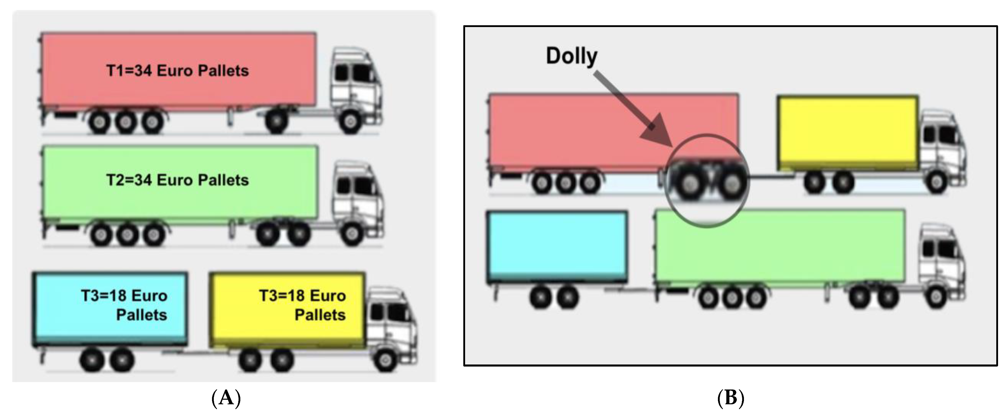
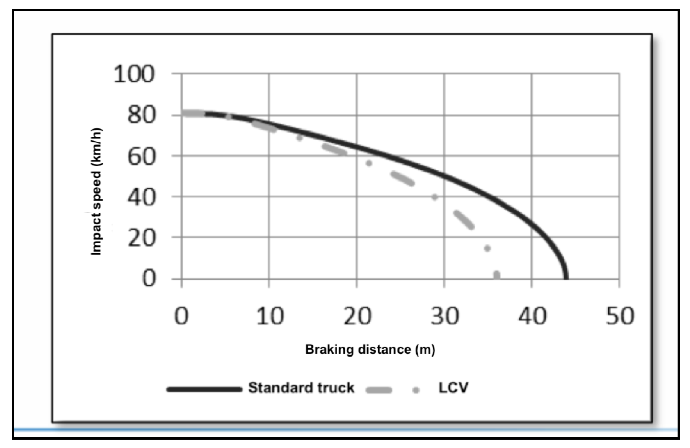
A long combination vehicle (LCV) is a combination of a standard heavy vehicle with an additional loading component, either a trailer or a swap body. Most of the components can be used in any road transportation fleet, resulting in low investment costs and low risk of failure. The advantages of LCVs are [1]: (i) a reduction in truck journeys, (ii) a decrease in fuel usage, (iii) savings regarding operating costs, (iv) less carbon footprint, and (v) a decrease in heavy vehicles on the highways. As for disadvantages, popular arguments against LCVs are the endangering of road safety and the damaging of infrastructure. Surprisingly, LCVs are even less harmful to the infrastructure compared to commercial trucks, because of a better weight lever on all axes. Also, the road safety increases through LCVs, since (due to extra wheels and corresponding brakes) their braking distance—from a speed of 80 km/h to standstill—is shorter by 19% compared to standard trucks (Süßmann (2015 [2]), see Figure 1). To illustrate, in Figure 2A the red semi-trailer $T_1$ has a braking distance of 44 m, but for the red-yellow combination in Figure 2B this is only 36 m.

Restrictions for implementing LCVs involve operational as well as technical requirements. As for the operational: (i) certain goods may not be transported (e.g., fluid bulk goods, dangerous goods, living animals), and (ii) drivers need to fulfil special requirements. An example of a technical requirement is an automatic axle load control system for all axles with pneumatic shock absorption.

Within Europe, LCVs started in Sweden and Finland (Forschungs Informations System, 2016 [3]). Since 1979, these countries have allowed truck combinations with a length of 24 m and a total weight of 60 tonnes. After Finland and Sweden, the Netherlands was the next country that implemented LCVs within their infrastructure. After several field tests, more EU countries followed.

LCVs are 6.5 m longer compared to standard European heavy vehicles with lengths of 18.75 m. The height of 4.0 m and width of 2.6 m are the same as for the standard European heavy vehicle. With the extra length, the loading capacity increases by 50% from 100 m³ up to 150 m³. Measuring it down for standard euro pallets it means that the storing capacity increases from 34 to 52 pallets (Mayer et al., 2013 [4]). The maximum weight of a loaded truck may differ per country from 40 t (Germany) to 60 t (Scandinavian countries, Spain, Netherlands, Belgium and Luxembourg).

2.1.1. Combining Standard Trucks into Long Combination Vehicles

Two LCVs can replace three standard European heavy vehicles, which considerably increases the loading capacity per truck. Let us illustrate how this combination may be done. Consider a factory $F$ located in the northern part of a certain country. From the factory—on a daily basis—palletized goods are delivered via heavy trucks to three customers $C_1$, $C_2$, and $C_3$. All three customers are located in the southern part of the country. In the present situation, every day, three separate standard trucks depart from the factory, each heading to one of the customers. Figure 2A depicts these trucks. Let trailer $T_i$ be heading for $C_i$, $i$ = 1,2,3. More precisely, let the loads for customer $C_1$ and $C_2$ be transported by the red and the green trailer, respectively, whereas customer $C_3$ is served by the two smaller ones having the colors blue and yellow. For brevity of writing, let us denote a truck with trailer(s) $T_i$ by truck $T_i.$

The three commercial trucks $T_1$, $T_2,$ and $T_3$ have already been successfully implemented on European roads over the past decades. To create an LCV out of them, we couple a trailer or semi-trailer on another heavy truck. Figure 2B shows the result. From the vehicles $T_1$, $T_2,$ and $T_3$ we create two LCVs, namely:

• The blue-green combination

A trailer (blue) will be connected to a semi-trailer (green) with an extra truck trailer hitch.

• The red-yellow combination

One semi-trailer (red) will be connected to a motor vehicle (yellow), a European heavy vehicle with a constructed enclosed loading capacity box. To realize this connection a dolly (see Figure 3) is required.

A dolly is an unpowered device to connect a truck unit with a trailer. It contains two axles with four wheels and a so-called fifth wheel, which is a semi-trailer coupling, situated on top as a disk. In Figure 2B the two extra axles added by connecting a dolly are encircled. For smooth handling, the dolly is standard equipped with a hydraulic steering system. The unique characteristic of the dolly is the rotatable drawbar and the self-steering front axle (Krone, 2017 [5]). This enables the mobility of the vehicle combination and distributes the wear of the tires. The purpose is to connect a semi-trailer to a motor vehicle and support the steering of such a long vehicle. The hydraulic steering dolly supports the driver of LCVs, especially in roundabouts and to avoid swinging out.

2.2. Hub and Spoke Networks

In ancient times, passengers as well as freight were transported in a direct way: from origin to destination. Then, in 1955, Delta Airlines launched a revolutionary idea: a hub and spoke (H&S) network. They organized traffic routes as a series of ‘spokes’ that connect outlying points to a central ‘hub’. Soon, the concept was embraced by the transport community.

An H&S network is defined as “a network to route products via a specific subset of links, rather than routing each product with a direct link from its origin to its destination point” (Contreras et al., 2010 [6], p. 392). An H&S network consists of one or more hub nodes to combine and reroute the flow of goods, resulting in a reduction of direct route links.

Economies of scale by consolidation of flows are a key motivation for H&S networks (Alumur et al., 2020 [7]). In such networks, the consolidation of flows increases the traffic density in many route segments. For a transportation setting, this greater traffic density allows for the using of larger and more cost-efficient vehicles (e.g., LCVs) with appropriate trip frequencies. The reduction of unit costs comes from sharing fixed costs over more units of demand, and possibly from using vehicles with lower variable costs. Switching to an H&S network offers a higher potential for increasing the customer pool by also considering customers with low quantities. Customer satisfaction will be increased, since—instead of multiple deliveries—only a single delivery has to be received (Chopra & Meindl, 2010 [8], p. 99). Additional benefits of H&S networks may come from increasing the frequencies of service on links (as a result of higher traffic density), and a better traffic balance across the network. Furthermore, hubs can concentrate administrative and technical resources, reducing operational costs and inventories.

A drawback of H&S networks (especially for perishable goods) is the longer transport time for the freight to be transported, because all goods will be first delivered to the hub. Moreover, hubs can be expensive: a facility needs to be built and maintained. Also, there are additional storage and labor costs.

In designing an H&S system “The aim is to find the location of hub nodes and the allocation of demand nodes to these located hub nodes” (Alumur et al., 2012 [9]). The challenge is to locate the hub facility and to connect the spoke nodes (non-hub) with the hub such that passengers/goods are delivered efficiently (Alumur & Kara, 2008 [10]).

This raises the problem of deciding whether to implement one hub node or multiple nodes (Parvaresh et al., 2014 [11]). Every hub node implies additional costs, such as fixed costs for establishing and maintaining a hub facility and variable costs for handling products (Rieck et al., 2014 [12]). In addition, disruption can harm hub facilities and lead to excessive costs [11].

To counteract disruption, it is worthwhile to design a more reliable hub network. Reliability in network theory is defined as “the ability of a system to perform well even when parts of the system have been failing” (Snyder & Daskin, 2005 [13]). In the transport service industry, new customers join the clientele and others leave on a frequent basis. This affects the route network of the transport provider and will also lead to additional costs. This is particularly true when hub facilities have been built and warehouse infrastructure has been installed.

2.3. Mobile Hub and Spoke Networks

In urban transport, mobile hubs are used as consolidation and transshipment points for last-mile parcel delivery (Faugère et al., 2020 [14]). These hubs are typically located at the neighborhood level. Multi-echelon networks for urban distribution have received a lot of attention in the academic literature (cf. Raicu et al., 2020 [15]), often using urban consolidation centers or urban distribution centers to bundle goods outside the boundaries of urban areas. A special case of an urban mobile hub is a mobile depot, which is a trailer fitted with a loading dock, warehousing facilities and an office. The trailer is used as a mobile inner-city base from where last-mile deliveries and first-mile pickups are done with electrically supported cyclocargos (Verlinde et al., 2014 [16]; Marujo et al., 2018 [17]). A recent study (Gerrits & Schuur, 2021 [18]) replaces cyclocargos by a combination of pedestrians, drones and street robots.

In (long haul) freight transport, the concept of mobile hubs is less well known. This paper introduces a specific concept of mobile hubs in order to align freight transport by (de)coupling trailers. To reduce costs and increase flexibility, we propose to switch from traditional fixed hub facilities to mobile hub facilities by using long combination vehicles. At the hub, standard trucks arrive to be merged into LCVs and, conversely, LCVs arrive to be split into standard vehicles. To this end, trailers and semi-trailers need to be loaded in a way that coupling and decoupling of trailers will replace the need of any fixed hub facility. In practice, the (de)coupling of trailers can be done on any sufficiently large parking lot along the highway. In this way, the location of a hub node is easily adjustable to any changes in the logistic demand, which leads to considerable savings in operational costs. This means that some important disadvantages of an H&S network mentioned in Section 2.2 disappear, since no hub facility needs to be built or maintained. Neither is there any additional storage and inherent labor cost. Section 3 and Section 4 elaborate on the mobile hub approach.

3. Materials and Methods

In this section, let us illustrate the concept of mobile hubs for long combination vehicles (LCVs) in a simple, abstract setting. Section 3.1 describes and analyzes the present situation. Section 3.2 explores two options for employing LCVs: (1) all customer locations are visited by LCVs, and (2) all customer locations are visited by standard trucks that have been decomposed from LCVs at a mobile hub. In Section 4, we employ the insights gained here in a real-life case study.

3.1. Present Situation

Let us reconsider the setting described in Section 2.1.1. Recall that from the (northern) factory $F$—on a daily basis—palletized goods are delivered via heavy trucks to the three (southern) customers $C_1$, $C_2$, and $C_3$. Every day, the three trucks $T_i$ (depicted in Figure 2A) depart from the factory, heading for $C_i$, $i$ $=$ 1,2,3, respectively. Let $C_1$ be the farthest customer. Furthermore, let $C_2$ be positioned to the east of $C_1$ and $C_3$ to the west. Initially, the trucks $T_2$ and $T_3$ will drive the same route as $T_1$, until one of them, say $T_3$, deviates. Let us denote the location where this happens by $P_1$. Later on, also $T_2$ deviates, say at location $P_2$. Figure 4 gives a schematic overview.

For convenience, we assume—in the present situation—for each of the three trucks the backward route (i.e., from customer to factory) to be the reverse of the forward route.

Let us denote the distances involved in the present situation as follows:

$$d(F,P_1)=x_1;d(P_1,P_2)=x_2;d(P_1,C_3)=z;d(P_2,C_1\left)=z_1;d(P_2,C_2\right)=z_2.$$

For our LCV discussion in Section 3.2, we need three more distances, which we denote as follows: $d$($P_2$, $C_3$) $=z_3$;$d$($C_3$, $C_1$) $=y_{31}$;$d$($C_3$,$C_2$) $=y_{32}$. For convenience, we assume throughout that all distances are symmetric, i.e., $d$($F$,$P_1$)$=d$($P_1$,$F$), etc. Note that the above construction of $P_1$ and $P_2$ entails that the shortest paths from the customers to the factory are given by: $C_1{P}_2{P}_{1}F,C_2{P}_2{P}_{1}F$ and $C_3{P}_{1}F.$.

Let $\alpha$ denote the cost per standard truck (including driver) per kilometer. Let FCPS denote the total forward costs, in the present situation, i.e., the total costs to travel from the factory to the customers.

From Figure 4 we see that

$$FCPS=\alpha \left(\left(x_1+z\right)+\left(x_1+x_2+z_1\right)+\left(x_1+x_2+z_2\right)\right)$$

(1)

The next section explores to what extent the present costs can be reduced by using LCVs.

3.2. Employing Long Combination Vehicles

Let us now explore the options for employing long combination vehicles (LCVs). In this case, the trailers depicted in Figure 2A are combined into the two LCVs depicted in Figure 2B. Hence, on a daily basis, two LCVs (each with one driver) depart from the factory.

Let $\beta$ denote the cost per LCV (including driver) per kilometer. Taking the fuel and maintenance into account, it is obvious that $\beta$ > $\alpha$. In the Appendix A

Table A1. Detailed cost breakdown for the actual and accurate costs (including driver) in € per km, both for a standard truck, as well as for a long combination vehicle.

, we perform a detailed analysis in order to derive the actual and accurate costs (including driver) in € per km. We use these in our case study. For now, it suffices to say that the difference between $\alpha$ and $\beta$ will be small, somewhere in the order of $\beta$ $=$ 1.05$\alpha$. Clearly, the relative benefit of using these two LCVs is maximal in the special case that the customer locations $C_1$, $C_2$, and $C_3$ coincide. Then, by construction, $P_1$ and $P_2$ coincide with the customer locations. Hence, the total costs for a roundtrip in the present situation are $6\alpha x_1$. Using LCVs leads to a total cost of $4\beta x_1$. So, estimating $\beta$ $=$1.05$\alpha$, we arrive at a cost reduction of 30%, which is to be seen as an upper bound for any cost reduction in our three customers example, regardless of the parameters. However, in practice, the customer locations may be further apart. Let us deal with that below. We consider two cases: (1) all customer locations are visited by LCVs, and (2) all customer locations are visited by standard trucks that have been decomposed from LCVs at a mobile hub.

3.2.1. Case 1: All Customer Locations Are Visited by LCVs

Let us assume that all customer locations are accessible by LCVs. Consider the two LCVs depicted in Figure 2B. Let us denote the upper one by LCV1 and the other by LCV2. Then LCV1 visits $C_1$ and $C_3$, whereas LCV2 visits $C_3$ and $C_2$. Since the distances are symmetric, orientation is no issue in finding the shortest routes. Clearly, a shortest route for LCV1 is $F{P}_1{C}_3{C}_1{P}_2{P}_{1}F$. It dominates the route $F{P}_1{P}_2{C}_3{C}_1{P}_2{P}_{1}F$ because of the triangle inequality. Similarly, $F{P}_1{C}_3{C}_2{P}_2{P}_{1}F$ is a shortest route for LCV2. Let CLCV denote the total costs of a pair of optimal round tours when all customer locations are visited by LCVs. From Figure 4 we see that

$$CLCV=\beta \left(2\left(2x_1+x_2+z\right)+\left(z_1+z_2\right)+\left(y_{31}+y_{32}\right)\right)$$

(2)

Let us compare this with the back-and-forth costs 2*FCPS of the present situation:

$$\begin{array}{cc}CLCV-2FCPS=& 2\left(\beta -\alpha \right)\left(2x_1+x_2+z\right)+(\beta -2\alpha )\left(z_1+z_2\right)\\ & -2\alpha \left(x_1+x_2\right)+\beta \left(y_{31}+y_{32}\right)\end{array}$$

By examining coefficients, we see that for $x_1$ large enough (and $\beta <1.5\alpha )$ this expression is negative, so that the LCV tours perform better than the present situation. On the other hand, if we shift customer location $C_3$ far enough to the left, then the large values of $y_{31}$ and $y_{32}$ render the expression positive. Hence, visiting all customers by LCVs is not generically cost improving. It is highly dependent on the parameter setting.

3.2.2. Case 2: All Customer Locations Are Visited by Standard Trucks Decomposed from LCVs at a Mobile Hub

Let us now explore the case when standard trucks are initially—at the factory—combined to LCVs, which drive a considerable distance, but are eventually, in the vicinity of the customers, broken down again into standard trucks heading for the customers. After serving the customers, the standard trucks reassemble and form LCVs that drive back to the factory. The rationale behind this seemingly complex process is either economical or practical (e.g., when LCVs are not allowed at the customer site). As for the preferred location for (de)composing LCVs, we opt for a mobile hub.

In this case, the trailers depicted in Figure 2A are initially divided over the two LCVs in Figure 2B. Hence, on a daily basis, two LCVs (with each one driver) depart from the factory, both heading to a mobile hub. At the mobile hub, the two LCVs are decomposed again into the three trucks of Figure 2A. The time to execute this is generally in the order of ten minutes, so it forms no impediment. Clearly, the decomposition into three trucks is only possible if there is a third driver and a towing vehicle at hand. Hence, two questions are to be answered: (i) How to organize a towing vehicle and a third driver? (ii) What is the best location of the mobile hub?

Towing Vehicle and Third Driver

It is common practice for transport companies to hire employees from different locations and provide them with a towing vehicle. So, they give those employees a towing vehicle and allow them to take that truck home with them. The advantage is that they can start driving directly from their home. To exemplify, consider a transport company located in Germany that has several customers in Great Britain. The German company has an English employee. That person is hired by the German company and has received a German towing vehicle but is located in Great Britain. British customers are served as follows. German drivers will bring a trailer with products demanded to a shipping company and leave the trailer there. After the shipping company has transported the trailer to Great Britain, the English employee will take over. He will pick up the trailer and start to deliver to all customers within Great Britain. When he is finished, he brings back the trailer to the harbor, leaves it there and drives home with the towing vehicle. A vessel will transport the trailer back to Germany, where German drivers will pick up the trailer and bring it to the home base.

The situation in our mobile hub case is similar. The transport company associated with the factory may handle the issue with the third driver and the towing vehicle as follows. They may hire an employee who lives (relatively) close to the hub point. They provide the driver with a towing vehicle, i.e., they bring the towing vehicle only once to the employee. From then on, the employee starts to work—on a daily basis—from the hub point instead of the home base factory in Hamburg. This can be arranged to be labor-cost-neutral, since one driver less is needed to go from Hamburg. The mobile hub approach gives the transport firm the possibility to even reach customers who are located far away, because the third driver starts his nine-hour driving from the hub point, whereas the other two drivers have been already driving from Hamburg to the hub point. Those two drivers lost at least four hours from the allowed nine hours (cf. Section 4.1) by driving down to the hub point.

As an alternative, we mention the option to hire a driver plus towing vehicle from an external company. It is not unusual to sell transport orders to other transport operators. Another alternative only works for customers in the vicinity of the hub. A third driver is not required. Just decouple the trailers. Then one of the two drivers takes one trailer and drives to the customers, drives back to the hub and picks up the second trailer to serve the customers. However, the latter alternative does not work for our case study.

Finding the Best Location of the Mobile Hub

One issue remains to be solved: what is the best location of the mobile hub? In the setting under discussion, it is easily verified geometrically that one may limit the search to only two candidates: the branch points $P_1$ and $P_2$. There is no absolute preference for one of them. The best choice depends on the parameter setting, as we show below. In evaluating the two hub choices, we have the following.

Mobile hub${\mathit{P}}_{\mathbf{1}}$

Let FCMH1 denote the total forward costs for a mobile hub at $P_1$ to reach all customers. From Figure 4 we see that

$$FCMH1=2\beta x_1+\alpha \left(z+\left(x_2+z_1\right)+\left(x_2+z_2\right)\right)$$

(3)

Hence, the present forward costs minus those in case of a mobile hub at $P_1$ are given by $FCPS-FCMH1=\left(3\alpha -2\beta \right)x_1$ > 0. Thus, this mobile hub choice is generically cost improving. This is remarkable since we saw in Section 3.2.1 that visiting all customers by LCVs is not generically cost improving. In a broader perspective, this result shows the following: whenever the shortest paths from the factory to the customers have an initial sub-path in common, then choosing the first branch point as a mobile hub is cost-improving. The larger the length of the common sub-path, the larger the cost improvement.

Mobile hub${\mathit{P}}_{\mathbf{2}}$

Let FCMH2 denote the total forward costs, for a mobile hub at $P_2$, to reach all customers. From Figure 4 we see that

$$FCMH2=2\beta \left(x_1+x_2\right)+\alpha \left(z_1+z_2+z_3\right)$$

(4)

Hence, the present forward costs minus those in case of a mobile hub at $P_2$ are given by F$CPS-FCMH2=\left(3\alpha -2\beta \right)x_1-2\left(\beta -\alpha \right)x_2+\alpha$($z-z_3)$. Note that this expression may have negative values. However, if $x_1$ is large, i.e., if the factory $F$ is sufficiently far from the first branch point $P_1$, then also this mobile hub case improves the current situation.

Note that

$$FCMH1-FCMH2=-2\left(\beta -\alpha \right)x_2+\alpha \left(z-z_3\right)$$

Hence, if $z\le z_3$ and $x_2>0,$ then $FCMH1<FCMH2$, in other words, then $P_1$ is preferred. Conversely, if $z>z_3$, then the sign of the right-hand side is indefinite. In this case, if $z$ is large enough to approach its triangular upper bound $x_2+z_3$, then the right-hand side is positive, so that $P_2$ is preferred.

3.2.3. Comparing Case 1 (‘All-LCV’) and Case 2 (‘Mobile Hub’)

Both cases have in common the fact that they start similarly: as LCVs from the factory. Case 1 is less general, since it assumes that every customer site is reachable by an LCV. Whether or not it is beneficial depends on the parameter setting. Case 2 requires more organization (e.g., hire—labor-cost-neutral—an employee who lives (relatively) close to the hub point and provide him with a towing vehicle (see our discussion in Section 3.2.2)). In addition, it requires the one-time purchase of a dolly (see Section 2.1.1). The costs of a dolly are modest. They are included in our LCV-costs analysis (see Appendix A Table A1).

Remarkably, a hub in $P_1$ is generically cost improving. When one compares the expressions (2)–(4) for the total costs $CLCV,$ 2*FCMH1 and 2*FCMH2, then it is obvious that none of them dominates. It all depends on the parameters. So, in a practical case, simply calculate each of the three expressions using the actual parameters and choose the (partial) LCV solution with the lowest costs.

Although out of scope in this paper, it may be worthwhile to augment the economic analysis with a risk analysis of the above choices. In particular, one may take into account that driving an LCV is safer than driving a standard truck, as seen in Figure 1. In addition, an LCV is less harmful to the infrastructure. Section 4 illustrates what additional complexity may arise in a real-life case.

4. Results

After having explored the concepts of LCVs and mobile hub networks in a simple abstract setting, let us now test our ideas in a real-life case study. To this end, we consider a company producing light technical items for industrial companies. We focus on the daily routes. Section 4.1 describes the current way of delivering to customers. Section 4.2 analyzes to what extent the abstract mobile hub approach of Section 3.2.2 is useful in this real-life case. Section 4.3 does the same for the all-LCV strategy.

4.1. Current Routes

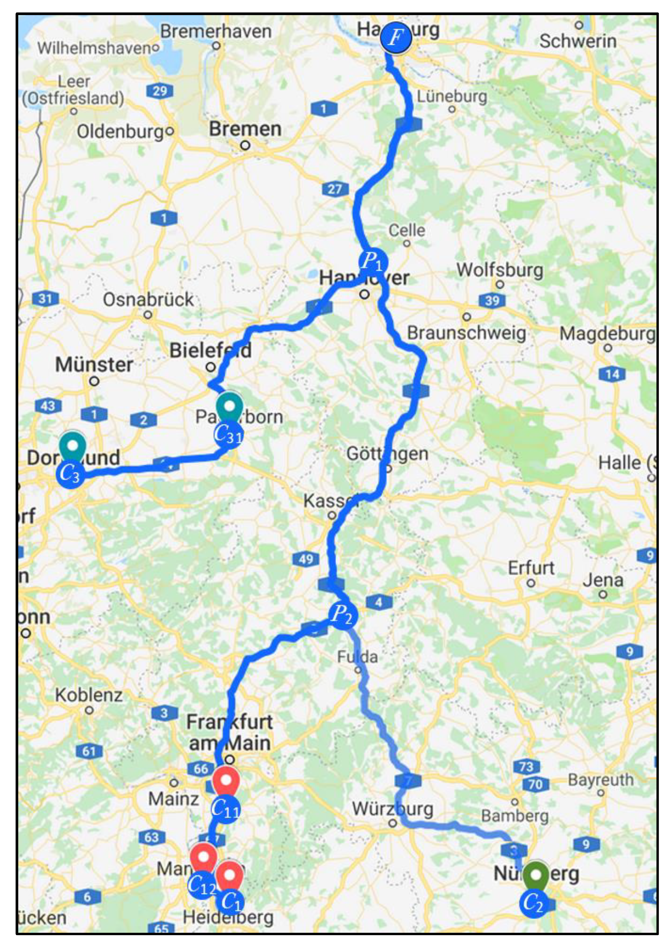
Figure 5 shows the factory location and the main customer locations. The factory $F$ is located in Hamburg. From there, the customers are currently delivered to via a heavy truck. The factory guarantees same-day delivery. In that respect, it is important to take notice of the EU rules on drivers’ hours (Regulation, 2020 [19]). These rules prescribe a maximum number of driving hours of nine hours in a day, which can be exceeded—up to 10 h—twice in a week. Hence, in the sequel, we will require that any route from $F$ to any of the customers will take at most 10 h of driving time.

In Figure 5, the various colored rings indicate the customers. Those who have the same color are currently delivered to by one truck, since this is cost-efficient. Thus, the three trucks $T_1$, $T_2$, and $T_3$, depicted in Figure 2A, leave Hamburg to drive in the same direction for delivering the items. Their routes are as follows:

First route (by truck $T_1$): Hamburg ($F$)- > Darmstadt ($C_{11}$) (9.6 pallets)- > Mannheim ($C_{12}$)(4.0 pallets)- > Heidelberg (${\mathit{C}}_{\mathbf{1}}$) (10.6 pallets)

Second route (by truck $T_2$): Hamburg ($F$)- > Nürnberg (${\mathit{C}}_{\mathbf{2}}$) (30 pallets)

Third route (by truck $T_3$): Hamburg ($F$)- > Paderborn ($C_{31}$) (15 pallets)- > Dortmund (${\mathit{C}}_{\mathbf{3}}$) (10 pallets).

For reasons of efficiency, the customers $C_{31}$ and $C_3$ are each served by different trailers. Obviously, there is an overlap of route driving by the three trucks. Initially, all trucks drive the same route, until one of them ($T_3$) deviates at the Hannover location. The other two proceed on the same route until they split up near Kassel. This gives us two candidates for mobile hubs: Hannover and Kassel.

Figure 6 shows the main road network corresponding to Figure 5 in a purely schematic way.

Indicated are the main highways connecting the case locations. In the present situation as well as in the mobile hub case (Section 4.2), we only employ the highways indicated by solid lines in Figure 6. In Section 4.3, where we analyze Case 1 (i.e., all customers are visited by LCVs), we may also employ the ‘dashed’ highways. In particular, the fastest LCV-connection from $C_3$ to $C_1$ is to go from $C_3$ to $C_{11},$ then from $C_{11}$ to $C_{12}$ and then from $C_{12}$ to $C_1.$

Comparing Figure 5 and Figure 6 with the (simplified) abstraction given by Figure 4, we readily identify abstract and concrete locations, as in

Table 1. Case locations with essential distances (in km) and driving times (in minutes).

		Km	Min		Km	Min
$F$$=$ Hamburg	$F$$-P_1$	127.0	126	$P_2$$-C_2$	301.4	223
$C_{11}$$=$ Darmstadt	$P_1$$-C_3$	236.4	171	$C_{11}$$-C_2$	255.7	245
$C_{12}$$=$ Mannheim	$P_1$$-C_{31}$	160.8	148	$C_{11}$$-C_{12}$$-C_1$	68.7	91
$C_1$$=$ Heidelberg	$P_1$$-P_2$	184.0	141	$x_1$$=$$F$$-P_1$	127.0	126
$C_2$$=$ Nürnberg	$C_{31}$$-C_3$	115.1	115	$x_2$$=$$P_1$$-P_2$	184.0	141
$C_{31}$$=$ Paderborn	$C_{31}$$-P_2$	91.1	89	$z$$=$$P_1$$-C_{31}$$-C_3$	275.9	263
$C_3$$=$ Dortmund	$C_3$$-P_2$	170.7	129	$z_1$$=$$P_2$$-C_{11}$$-C_{12}$$-C_1$	289.1	294
$P_1$$=$ Hannover	$C_3$$-C_{11}$	257.7	250	$z_2$$=$$P_2$$-C_2$	301.4	223
$P_2$$=$ Kassel	$P_2$$-C_{11}$	220.4	203	$z_3$$=P_2$$-C_{31}$$-C_3$	206.2	204

.

One may wonder what is the fastest LCV-connection from $C_3$ to $C_2$. Figure 6 gives us two options: $C_3{C}_{11}{C}_2$ and $C_3{P}_2{C}_2$. Table 1 tells us that $C_3{P}_2{C}_2$ is the fastest.

4.2. Mobile Hub Analysis

Let us now analyze to what extent our mobile hub approach (Case 2, described in Section 3.2.2) is useful in the real-life case described above.

4.2.1. Mobile Hub: Distance and Cost Analysis

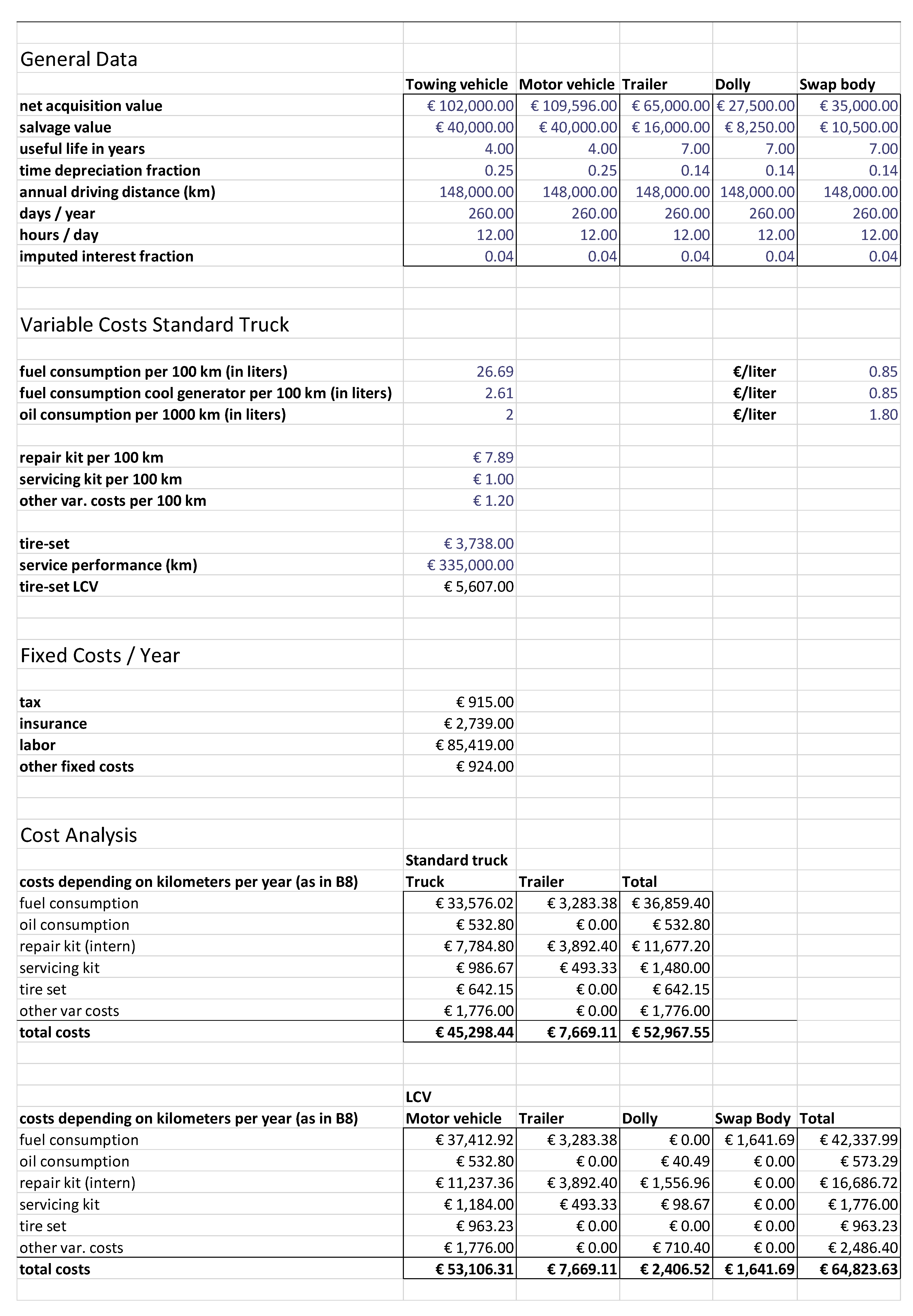
In the Appendix A Table A1, we perform a detailed analysis in order to derive the actual and accurate costs (including driver) in € per km. Both for a standard truck, as well as for an LCV, we perform an elaborate calculation in order to obtain the annual (i) driver labor costs (ii) fixed costs and (iii) km-dependent costs (such as fuel, tires, repair kit). Dividing the total of these costs by the annual driving distance we find the following costs—including driver (and for the LCV including dolly)—in € per km:

For a standard truck: $\alpha$ $=$ 1.12507

For an LCV: $\beta =1.28030$

Table 1 gives us the values of the distances $x_i,z_j$ and $z.$ Hence, we have gathered all data needed to apply our comparison. Using the formulas (1), (3), and (4) we find:

Total costs to reach all customers in the present situation: FCPS = € 1817.4

Total costs to reach all customers with a mobile hub in Hannover: FCMH1 = € 1713

Total costs to reach all customers with a mobile hub in Kassel: FCMH2 = € 1692.7

Hence, cost-wise, the best choice for a mobile hub is Kassel, as depicted in Figure 7. The reduction in cost, relative to the present situation, is (FCPS-FCMH2)/FCPS = 0.0686. One may argue that a cost reduction of only 7% is not worth the trouble. However, in road transport, business margins are extremely small, which certainly makes the idea of mobile hubs worthwhile.

4.2.2. Mobile Hub: Time Analysis

Let us check whether the routes considered in Section 4.2.1 are in agreement with the EU rules [19], i.e., not taking any longer than 600 min (allowed twice per week), but preferably no longer than 540 (allowed on a daily basis).

In the present situation, using the data from Table 1, the driving time (in min) to reach the farthest customers $C_1$, $C_2$ and $C_3$—via the customers in between—is found to be 561, 490 and 389, respectively. Hence, all three drivers obey the rules. However, since it takes more than 540 min to reach customer $C_1$, a specific driver is only admitted to drive the route $F{C}_1$— or $C_{1}F$—at most twice a week.

Next, let us consider the case of a mobile hub in Kassel ($P_2)$. Then driver 1 and driver 2 start off from Hamburg $\left(F\right)$ and drive their LCVs for 267 min to $P_2$. At the hub $P_2$ they meet driver 3. From $P_2$, the three drivers have to be assigned to the three (subsequent) routes: to $C_1$, $C_2$ and $C_3$—via the customers in between—taking 294, 223 and 204 min of driving time, respectively. It makes sense to assign the longest route to driver 3, assuming he drove less than the other two drivers. The other drivers will then have driven in total 490 and 471 min when arriving at the farthest customer. Consequently, all three drivers are driving less than 540 min. Hence, the EU rules allow these routes every day of the week.

4.3. Analysis of the All-LCV-Strategy

Let us assume that all customer locations are accessible by LCVs. Consider the two LCVs depicted in Figure 2B. From these, LCV1 visits: (i) $C_{11},C_{12}\mathrm{and}{C}_1$ and (ii) either $C_{31}\mathrm{or}{C}_3$. Complementary to that, LCV2 visits $C_2$ and either $C_{31}\mathrm{or}{C}_3.$

4.3.1. The All-LCV-Strategy: Distance and Cost Analysis

Table 2. The shortest routes for the all-LCV-strategy.

	Forward Route	Backward Route	Total Distance Per LCV
LCV1 visits C31	F P1 C31 P2 C11 C12 C1	C1 C12 C11 P2 P1 F		total distance
distance (km)	668	600.1	1268.1	2716 km
LCV2 visits C3	F P1 C3 P2 C2	C2 P2 P1 F		total costs
distance (km)	835.5	612.4	1447.9	€ 3477.3
LCV1 visits C3	F P1 C3 C11 C12 C1	C1 C12 C11 P2 P1 F		total distance
distance (km)	689.8	600.1	1289.9	2582.6 km
LCV2 visits C31	F P1 C31 P2 C2	C2 P2 P1 F		total costs
distance (km)	680.3	612.4	1292.7	€ 3306.5

gives the shortest routes corresponding to the two cases mentioned in the previous paragraph.

So, the best option is to let LCV1 visit $C_3$ and LCV2 visit $C_{31}$. The corresponding costs are € 3306.5. In Section 4.2 we found for the best mobile hub option (a mobile hub in Kassel) the costs 2*FCMH2 $=$ € 3385.4. So, the all-LCV-strategy is the cheapest here, provided the EU rules are obeyed. Let us check those in Section 4.3.2.

One of the reasons that the all-LCV-strategy outperforms the mobile hub strategy cost-wise is the following. The road network in our case study is extremely dense, so that convenient short-cuts for LCVs are possible. Let us illustrate what happens if the road network is coarser. Suppose there is no direct connection between $C_3$ and $C_{11}$. Suppose that, instead, one drives from $C_3$ to $P_2$ to $C_{11}$. Then, in Table 2, all routes stay the same, except for one. When LCV1 visits $C_3$, then the forward route $F{P}_1{C}_3{C}_{11}{C}_{12}{C}_1$ with the distance of 689.8 km is replaced by the route $F{P}_1{C}_3{P}_2{C}_{11}{C}_{12}{C}_1$ with the distance 823.2 km. In that case, each of the LCVs drives a distance of 2716 km. Consequently, the all-LCV-strategy has lowest costs at € 3477.3, which is worse than the best mobile hub option with costs 2*FCMH2 $=$ € 3385.4.

4.3.2. The All-LCV-Strategy: Time Analysis

Let us consider the (best) option—LCV1 visits $C_3$ and LCV2 visits $C_{31}$—and check whether the associated forward routes are in agreement with the EU rules, i.e., not taking any longer than 600 min. Using Table 1, we find that—to reach all customers—the LCV1 driver drives 638 min and the other 586 min. Hence, this option violates the EU rules. The next-best option—LCV1 visits $C_{31}$ and LCV2 visit $C_3$—violates the EU rules as well. In trying to achieve same-day delivery, one might be tempted to go for an intentional light violation of the EU rules, e.g., by structurally driving several minutes longer than allowed. However, the Working Time Act (2008 [20]) sees this as endangering an employee’s health which is punishable by imprisonment of up to six months. We conclude that, surprisingly, the optimal time-feasible solution to the case problem is to use a mobile hub in Kassel ($P_2)$.

5. Discussion

Basic for the analysis in our paper is the fact that LCVs have an additional loading capacity of 50% compared to standard trucks. We have been calculating different options to find cost-efficient and time-feasible LCV routing strategies. We concentrated on two methods in greater detail: ‘mobile hub’ versus ‘all-LCV’. We saw that both approaches have advantages and disadvantages. Let us elaborate further on those in this section.

The main advantage of a mobile hub network is that it is flexible and that the radius of same-day delivery is large. It is easily adjustable to meet customer requirements, such as (un)loading times. Due to same-day delivery and just in time requirements, customers change their order volumes on short notice. Also, traffic jams or illness of the driver are aspects that can influence time delivery. In a mobile hub network, it is possible to react to those obstructions by first transporting the goods to a hub and then dividing the freight over other trailers. This allows us to extend the number of customers on the route. New customers on the same route can be delivered to as well.

The mobile hub network also has disadvantages. An additional driver and a towing vehicle are needed at the hub. However, since one less driver and one less towing vehicle are needed at Hamburg, the transport company may stay labor-cost-neutral and hire an employee who lives (relatively) close to the hub point and provide him with a towing vehicle. The only equipment investment needed is the one-time purchase of a dolly, which is quite modest (see the Appendix A Table A1, where we included the dolly in our LCV-costs analysis). As in cross-dock systems, the logistic players involved must be linked with fast ICT to ensure that all pickups and deliveries are made within the required time windows (Simchi-Levi et al., 2007 [21], p. 233).

In the other method “all-LCV”, we just use our LCVs and try to serve as many customers as possible. The advantages are that fewer employees and trucks are needed. In this case, we don’t need a third driver and an additional towing vehicle. Therefore, it yields a better use of volume per truck and fewer expenses. The negative aspect of all-LCV is the time. The (daily) driver is only allowed to drive nine hours per day. This limits the number of customers that can be reached in a forward route within the same day.

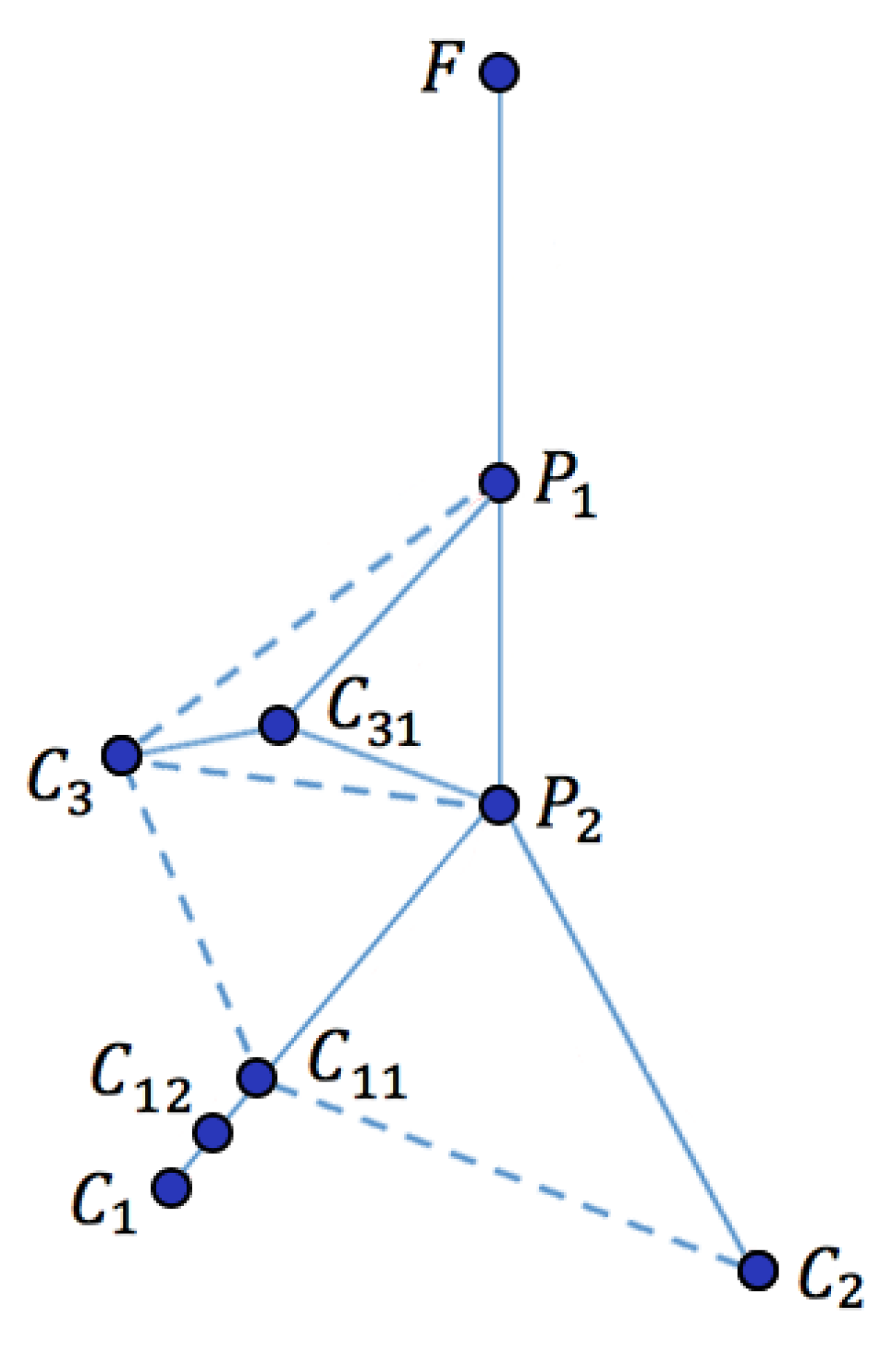
Our study focuses on three routes. Let us briefly dwell on the general situation. Consider a company that currently only uses standard trucks. The company may wonder whether or not it is beneficial to employ a mobile hub system. To support a decision, it would be worthwhile to have a lower bound for the cost improvement potential. To provide such a lower bound, let us give a simple procedure to construct a specific mobile hub configuration for the company. Obviously, this configuration can be improved by smart heuristics. Our procedure can be carried out by any planner using standard planning tools. It runs as follows:

• Cluster adjacent customers into trailer loads. Let $C_i$ denote the resulting customer clusters.
• For each customer cluster $C_i$, determine the shortest path $P_i$ from the factory to the cluster.
• Group the paths $P_i$ into path groups $G_j$ such that the paths in each group share a substantial initial sub-path of length $s_j$. (If need be, slightly deform the paths to accomplish this.) Let $n_j$ be the number of paths in $G_j$.
• For each path group $G_j$, determine an appropriate number ${\ell }_j$ of LCVs that can be decomposed into the $n_j$ standard trucks.

Then a lower bound for forward cost improvement (from using standard trucks into using the mobile hub concept) is given by: ${\displaystyle \sum }_j(n_j\alpha -{\ell }_j\beta )s_j$.

Proof. 

Put a mobile hub at the end of each initial sub-path (at distance $s_j$ from the factory). After the LCVs are decomposed at the hubs, standard trucks emerge that drive the same routes as in the current situation. Only the situation before the hub is different: instead of $n_j$ standard trucks with associated forward costs $n_j\alpha s_j$, we now have ${\ell }_j$ LCVs with associated forward costs ${\ell }_j\beta s_j.$ Since this hub choice is only one of the many options possible, the resulting summation is a lower bound on the forward cost improvement potential. □

6. Conclusions

This paper aims to develop a generic transport system suitable for matching long-distance bulk distribution with local distribution. To this end, we introduce the concept of a mobile hub (MH) network in combination with long combination vehicles (LCVs). Mobile hubs allow for the switching of trailers at any suitable location at any time. Therefore, they increase flexibility and yield savings in time and costs. Driver hours—a scarce good nowadays—are reduced as well. In our LCV-MH concept, standard trucks are initially—at their home base—combined with LCVs, which drive a considerable distance but are eventually, at a mobile hub in the vicinity of the customers, broken down again into standard trucks heading for the customers.

We illustrate the LCV-MH concept in a simple, abstract setting. In this setting we compare the concept with the all-LCV strategy where one uses only LCVs to serve the customers. We employ the insights gained in a real-life case study. In the latter, we focus on three routes, each from the factory in Hamburg to different customer clusters in Southern Germany. The routes are currently driven by standard trucks. When employing the all-LCV strategy, we find that the routes generated violate the EU transport rules. The optimal time-feasible solution to the case problem is obtained by applying LCV-MH (with a mobile hub in Kassel). It yields a cost reduction of 7%. Since, in road transport, business margins are extremely small, this makes the idea of mobile hubs worthwhile.

Our real-life case study focuses on three routes. The latter situation may be conceived as ‘atomic’. In general, the LCV-MH concept can be applied to any number of routes yielding a considerable reduction in costs and driver hours. When calculating different options to find the best solution, an essential issue one has to deal with is the number of driver hours and the requirements of the customer. With the mobile hub network, we were able to fulfil customer requirements while taking into account driver regulations. The mobile hub concept does not involve major investments and is also not dependent on any location. Moreover, in the foreseeable future, when trucks are driving autonomously, the LCV-MH concept will prove to be even more fruitful and robust, since the dependence on human drivers vanishes. In fact, the LCV-MH concept may even accelerate these technological changes, since the currently extremely scarce driver can be replaced by an autonomous system on the easily drivable main highways from the factory to the hub. Using truck platooning, the autonomously driving LCVs can reach the summit of efficiency.