Abstract
Workpiece location is critical to efficiently plan actions downstream in manufacturing processes. In labor-intensive heavy industries, like construction and shipbuilding, multiple stakeholders interact, stack and move workpieces in the absence of any system to log such actions. While track-by-detection approaches rely on sensing technologies such as Radio Frequency Identification (RFID) and Global Positioning System (GPS), cluttered environments and stacks of workpieces pose several limitations to their adaptation. These challenges limit the usage of such technology to presenting the last known position of a workpiece with no further guidance on a search strategy. In this work we show that a multi-hypothesis tracking approach that models human reasoning can provide a search strategy based on available observations of a workpiece. We show that inventory tracking problems under uncertainty can be approached like probabilistic inference approaches in localization to detect, estimate and update the belief of the workpiece locations. We present a practical Internet-of-Things (IoT) framework for information collection over which we build our reasoning. We also present the ability of our system to accommodate additional constraints to prune search locations. Finally, in our experiments we show that our approach can provide a significant reduction against the conventional search for missing workpieces, of up to 80% in workpieces to visit and 60% in distance traveled. In our experiments we highlight the critical nature of identifying stacking events and inferring locations using reasoning to aid searches even when direct observation of a workpiece is not available.
1. Introduction
Information of the state of various materials and processes within the shop-floor is critical to improve process efficiency in any manufacturing environment. This is reflected in the framework prescribed by the fourth industrial revolution, Industry 4.0, which is rooted in IoT (Internet of Things), which vastly expands the scope of available information for a process [1,2,3]. Information on the location of raw materials, process states or the state of any component that plays a part in the shop-floor is necessary to build a Digital Twin (DT) or a Cyber Physical System (CPS) [4,5] that presents a snapshot or model of the current state of the entire process pipeline. Availability of such DT or CPS of the shop-floor can help bridge the gap between the expected state of elements that workers plan tasks on, as well as the actual state [6,7] that is affected by various other agents and actors within the system. In the absence of such a system and given that any worker cannot manually monitor and account for the effect of every other actor, uncertainty creeps into process plans, creating unnecessary delays. Manufacturing industries that have adopted the Industry 4.0 framework have shown significant improvements in efficiency, and the manufacturing sector overall has since shown a healthy 6% annual growth rate [8]. However, heavy manufacturing industries, like construction and shipbuilding, face several challenges in adopting Industry 4.0 concepts [9] and show only a 2% growth, trailing far behind the industry average.
Construction and shipbuilding industries, though considered to be a part of the manufacturing industry sector, present very different work environments compared to the rest of the industry [10,11]. One significant difference here is that tasks move around the product, whereas products move around tasks in most of the manufacturing industries like those involved in mass-manufacturing. This makes it difficult to adopt sensing and automation technology that was matured within the manufacturing industry sector, as the fundamental process structure is incompatible. This is particularly evident in the inventory tracking front, which is necessary to build a CPS of the project.
Besides the lack of a CPS, nearly 50–60% of the entire project cost in these industries is spent on raw materials [12] that are consumed directly or after further processing. Since materials are consumed while the workspace is evolving, it limits available storage options. This makes it impractical to build structured storage solutions on-site for all the raw materials and leads to workpieces being stacked on by multiple stakeholders in the project. Long storage times, handling by multiple stakeholders and accidental displacement combined with the lack of an effortless information collection solution to log any displacements leads to poor pull times in these environments [4,8,13,14,15]. Since workpiece displacement and movement decisions are not centralized and occur locally at worker’s discretion, we focus on collecting information from their point of view and extracting the effect of such displacement decisions downstream through a reasoning model. The purpose of our proposed system is to reduce effort and time spent in searching for workpieces without adding any additional cognitive burden on the movers during workpiece displacements, accidental or otherwise.
The remainder of this article is divided into four sections. Section 2 discusses current work in literature that directly tackle the inventory tracking problem and those that deal with probabilistic and reasoning-based methods in the field of robotics from which we draw concepts. Section 3 describes the motivation and design of various components of our proposed approach, focusing on the contributions over our previous work [15]. Section 4 covers the setup, design and results for the experiments conducted to validate our approach. Finally, Section 5 discusses the conclusion, limits, and future work for our system.
2. Related Work
The prevalence of the inventory tracking problem in the shipbuilding and construction industries and the reasons for it are well-documented in the literature. A review of current shop-floor practices and cost of lost inventory to the entire process pipeline has been highlighted in [8,10,13,16]. A field review of a construction site by [4] highlighted the limitations in manual logging of inventory in terms of time spent on searching for lost inventory. They further showed that with an automated information collection system, processes showed significant reductions in completion time. Apart from documenting the problem and its causes, there are several suggested solutions for an information collection system to maintain up-to-date information on inventory movement [17,18] using techniques and sensors similar to those used in warehousing and mass-manufacturing industries. To our knowledge, previous work addressing the problem of inventory tracking in the construction and shipbuilding industries focused on modes of information collection. While these methods suggest solutions that are based on a track-by-detection approach, they break down in the absence of detection, which is common in cluttered and stacked environments. Our proposed approach explicitly relays ambiguities and borrows from a wider stream of research areas that deal with uncertainties, such as robotics and probabilistic modeling. While information collection is an integral part of our proposed approach, we expand on available information to provide suggestions in the absence of direct detection a workpiece. In our approach, apart from information collection, we employ a probabilistic multi-hypothesis approach to provide suggestions on workpiece location.
Information collection: Information collection is described as one of the building blocks of the Industry 4.0 paradigm. The need for such a system in industries operating in unstructured environments has been identified as one of the essential steps towards improving process efficiency and faster pull times [1,2,5,10,17]. While the need is well established, current research thrust, to our knowledge, is focused on improvements to and adaptation of current Radio Frequency Identification (RFID) technology [16,18,19,20]. With the warehousing industry pushing for RFID to be a standard mode of information collection, implementation costs have been reduced, making it more attractive for adoption by the construction and shipbuilding industries [21]. Since placing, logging, and pulling inventory are the primary purposes of warehouse workers, time spent in making sure inventory locations get registered through RFIDs is well justified. However, in the construction and shipbuilding industries, to further reduce burden to human workers, the authors of [22,23] explored an autonomous information collection system using drones with RFID and vision sensors to detect RFID and barcodes or Augmented Reality (AR) tags. Apart from detection based on AR tags and barcodes, recently, computer-vision based information collection methods have been explored as an alternate. Work by [24,25,26] explored the idea of using current state-of-the-art detection methods in computer vision to track specific events involving heavy machinery, equipment and personnel to actionable information so as to improve safety and track heavy equipment movement throughout work sites.
While the objective of our system of improving inventory pull times without adding additional cognitive burden to workers is similar to the methods described here, the final information presented is based on tracking-by-detection. However, unstructured environments where workpieces are cluttered and stacked pose several challenges to detection by RFID and vision-based systems. While RFID does not need line-of-sight for detection, the penetration limits of the interrogation signal in passive RFID-based detection make for poor information collection [5,27]. While active RFID-based detection provides better detection, they pose several cost and implementation challenges for stacks of heavy and abrasive workpieces that are common in workspaces. These challenges make detection quite difficult in these environments, limiting the usefulness of a tracking-by-detection approach. In our approach, we further expand on available information to identify multiple case scenarios as hypotheses and propagate and prune them to provide actionable information to guide search for missing inventory.
Probabilistic tracking: Probabilistic approaches to meter ambiguities in detections and robot states have been successful in research as well as practical applications in the field of robotics. For example, in particle filters [28], a popular method to track objects in images, multiple hypotheses as particles are populated to span possible locations in the hypothesis space. The weight or confidence in each of these particles is updated based on its fit to incoming observations. These approaches employ a Bayesian inference-based approach to make sequential observations while updating their estimate of state, given some model of the environment to correlate observations. While these approaches have been quite popular in the areas of robot localization [29,30] and computer vision, to our knowledge, there has been little work exploring such techniques that provide actionable information while preserving ambiguity for inventory tracking applications. In our work we show that these concepts can be customized for the purposes of inventory tracking by providing a model for identifying stacking events that could occur, from observations of workers interacting with workpieces.
Multi-hypothesis tracking: Multi-hypothesis tracking approaches [31] gained popularity in the early 1990’s as a solution for data-association problems that involved ambiguities in detections and sensor readings. These methods required maintaining multiple hypotheses, as tracklets, where a graph of each hypothesis is spawned, updated, and pruned, so as to avoid strict pairwise data associations over time until ambiguities could be resolved from further observations. In recent years, improvements in sensor and detection algorithm accuracy have shifted focus away from these approaches [32]. However, they present an ideal framework to incorporate complex higher-order information into tracking when detection cannot be guaranteed due to occlusions and stacking, as is the case for inventory in unstructured storage environments.
Reasoning-based inference: Reasoning-based methods aim to model relations between events and actions and try to extract deeper inferences such as intent. Such methods aim to build causal relations between observed events through grammar defined as first order logic [33] or as probabilistic causal graphs [34]. These methods infer useful outcomes from observations through first order logic or event outcome maps that are solicited from human knowledge. Most algorithms expand this knowledge by further discovering patterns from observed events and outcomes. While these methods have been popular in cognitive science and artificial intelligence, to our knowledge, there is little work exploring their usage in industrial applications such as inventory tracking. Recently, work by [35] has shown that these methods can be adapted for use in real-world object tracking applications to determine the location or state of occluded pedestrians, expanding the scope of track-by-detection algorithms. Work by [36] has also shown that such methods can be used to predict intent and upcoming actions in scenarios if expert knowledge that models the behavior of the world is available. Such algorithms that build on causal grammar provide promising results to infer the hidden states of objects that are not otherwise visible, conditioned on the context set by the immediate environment. Since one of the challenges in inventory tracking is occlusion or lack of direct observation, we employ similar reasoning, to expand the hypothesis for workpiece location even when direct observations of a workpiece are not available.
3. Proposed Approach
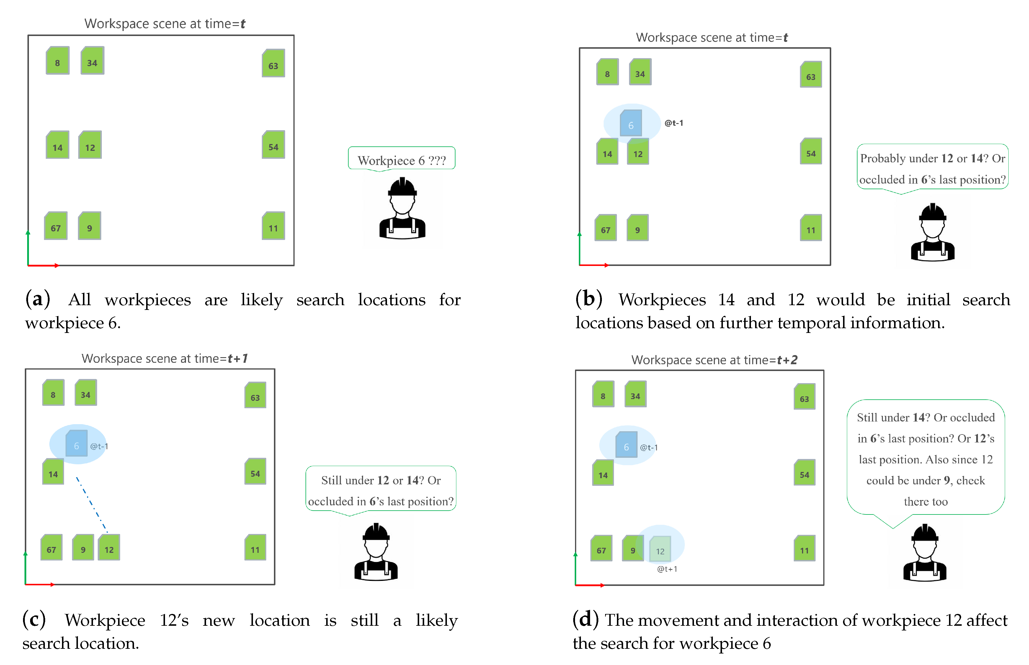
Our proposed approach aims to reason possible locations of workpieces as an effect of events that have taken place leading up to losing track of the workpiece locations. The reasoning model described in our approach mirrors the reasoning a human worker would follow to build a search strategy when given enough observations and time. For example, as shown in Figure 1a, given a snapshot of the state of workpieces in the workspace at any time t, one cannot do better than a random guess on the location of the missing workpiece 6. However, given its last-known-position in the workspace at (Figure 1b) and further events in time (Figure 1c,d), the search strategy propagates based on the worker’s knowledge of the physical world and workpiece movement. In our approach we try to model this behavior of building a search strategy for missing workpieces based on observed events involving the workpiece. To accomplish this, we need two critical components as shown in Figure 1: an information collection system (Section 3.1) to present the observable workpiece scene across time; and a reasoning model (Section 3.2), similar to that of a worker, to infer possible locations and propagation of stacks.
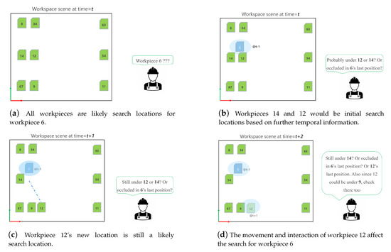
Figure 1.
A scene representing a worker’s reasoning to decide on search locations given temporal location information. (a)With just the current snapshot of the workspace, search for a workpiece defaults to chance for any worker. (b) Information on events leading up to the disappearance of workpiece 6, however, immediately introduces priority search locations of workpieces 12 and 14 based on simple reasoning of proximity. (c) The search strategy evolves along with the movement of workpieces as the initial suspected stack location, workpiece 12, is moved (d) This process can be chained with further changes in workpieces based on workers’ reasoning for the propagation of stacks.
This work expands on our previous work described in [15] and focuses on addressing its limitation to prune search locations and extract more critical events from movers (Section 3.5). We also present methods to provide tighter search locations through knowledge insertion (Section 3.2), if available. While our previous work gives a detailed visual description of stack propagation and the concurrent operations in the event and dependency graphs, in this article we limit the discussion to strengthening our proposed approach by providing underlying probabilistic principles and additional contributions of this work. In the interest of completeness, algorithms for building and evolving each graph are described in Appendix A1.
The remainder of this section covers the components involved in the proposed approach. The system is built following a modular design that allows for each component to be swapped out or configured independently as the environment demands. Section 3.1 describes the hardware and IoT-driven architecture used for information collection. Section 3.2 describes the underlying formulation based on discrete Bayesian inference, commonly employed in Markov localization methods [29], which is used to build probabilistic relations between workpieces. We show how observations are correlated to a model, based on expert knowledge of workpiece movement and stacking, to calculate weights for said relations.
3.1. Information Collection
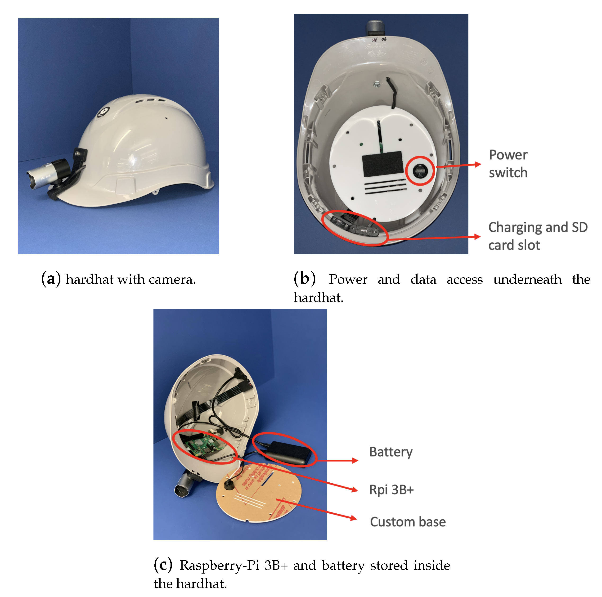
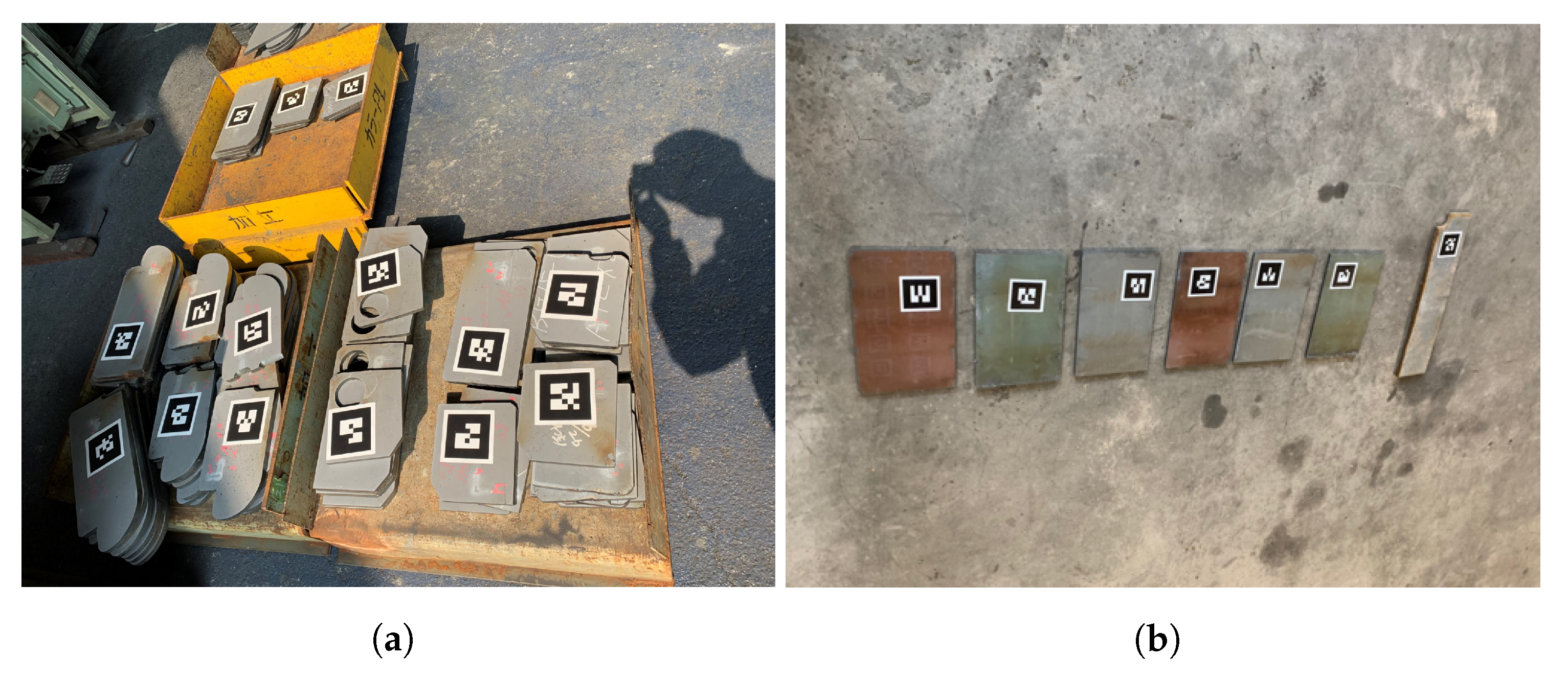
The objective of the information collection module is to present the scene of observable workpieces through workers and fixed cameras at any time (Figure 1). This module presents the observable scene of the workspace across time for the reasoning module to build the beliefs for missing workpieces. In our system, we use wired USB-cameras to capture and transfer images to Raspberry-Pis attached to workers’ helmets (Figure 2) and machinery such as forklifts, collectively referred to as movers. As multiple movers move around the workspace to interact and displace workpieces, this module publishes images from their view at 30 frames per second (FPS). These images represent the raw data from which workpieces tagged with Augmented Reality (AR) markers (Figure 3) and events are identified by the detection and reasoning modules, respectively.
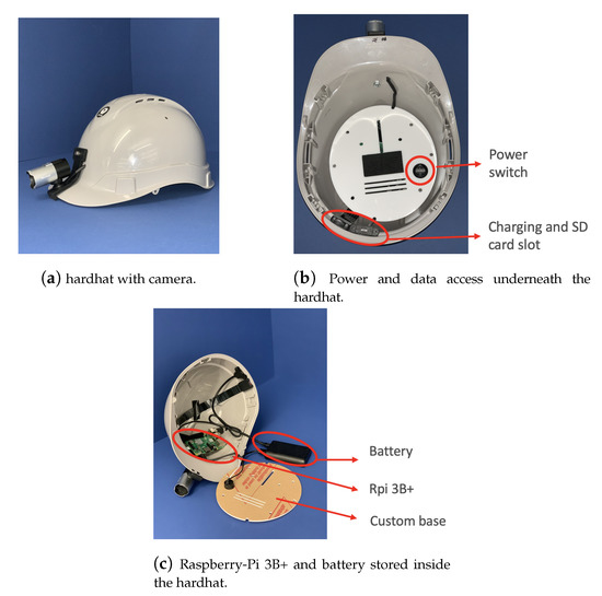
Figure 2.
Cameras attached to a worker’s gear to observe the immediate environment. (a) A worker’s helmet fitted with USB cameras to provide the field of view of the worker to our system. (b) Easy access to power switches, charging ports and an SD card slot allows for quick access and charging when the hardhat is not in use. (c) Internally, the hardhat houses the battery and Raspberry-Pi. This allows each mover to behave as an IoT device for information collection.
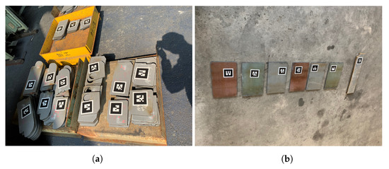
Figure 3.
Workpieces tagged with AR markers used for experiments at the shipyard. (a) Real-world workpieces within the shipyard viewed by a worker. (b) Test environment where the workpieces were moved by workers to evaluate our system under real-world mover behavior.
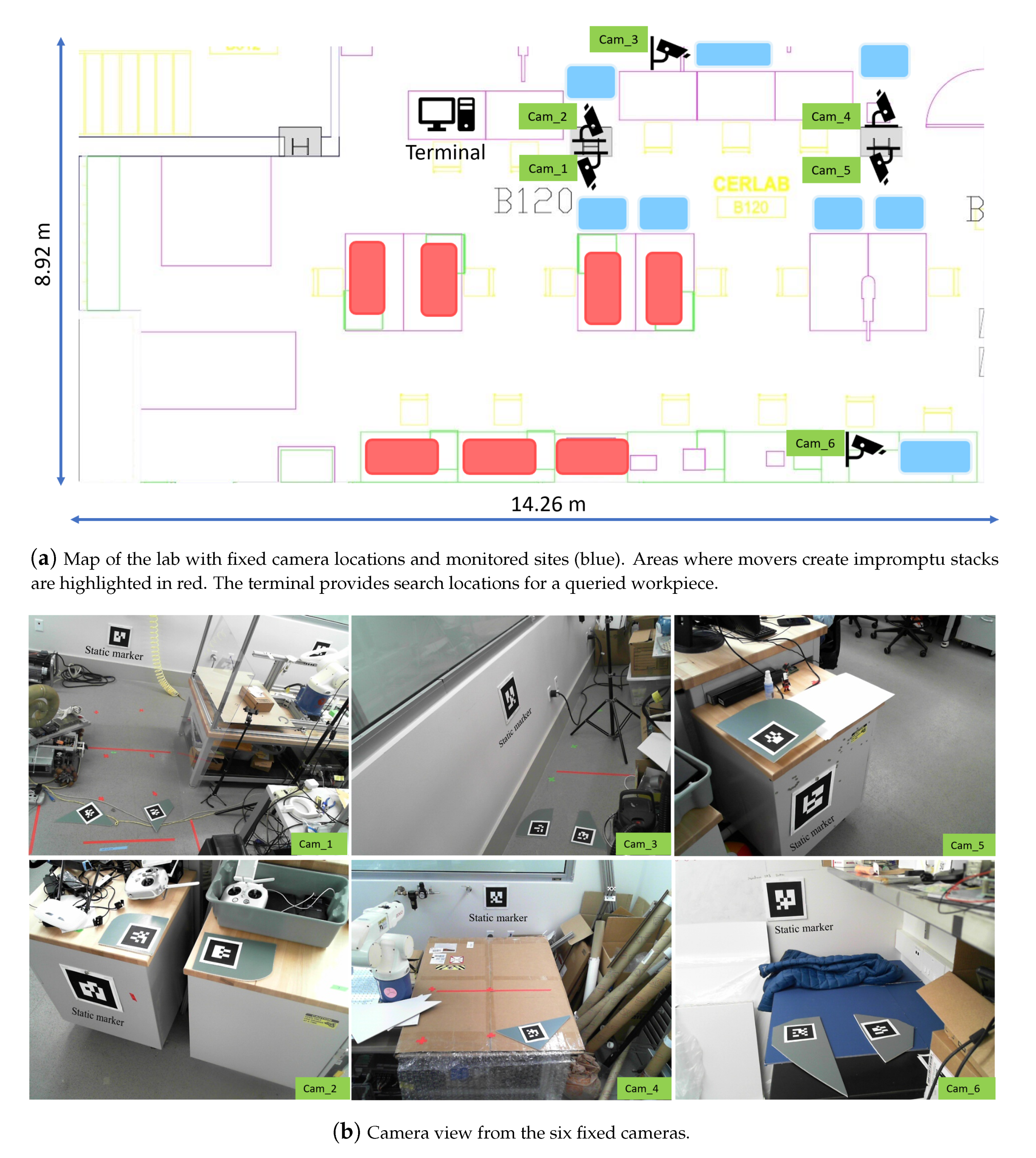
AR marker setup: Static AR markers of known pose (translation and rotation) with respect to a predefined workspace origin are placed in expected storage locations. When observed, these AR markers provide the pose of the observer with respect to the workspace. While static AR markers localize the observer with respect to the workspace, workpieces tagged with AR markers localize the workpieces with respect to the observer. If the observer’s location is known, the location of the observed workpiece is calculated through chained transforms between workpiece and observer and observer and workspace. Locations for the placement of static AR markers can be determined based on the field of view of fixed cameras placed throughout the workspace monitoring likely storage locations. (Figure 4). While we use AR markers as the mode of detection for our work, any mode of detection that provides location and identity (ID) of the workpiece can be used in its place. The focus of our work is on inferring locations of stacked workpieces when a direct observation of workpieces, through any mode of detection, is unavailable.
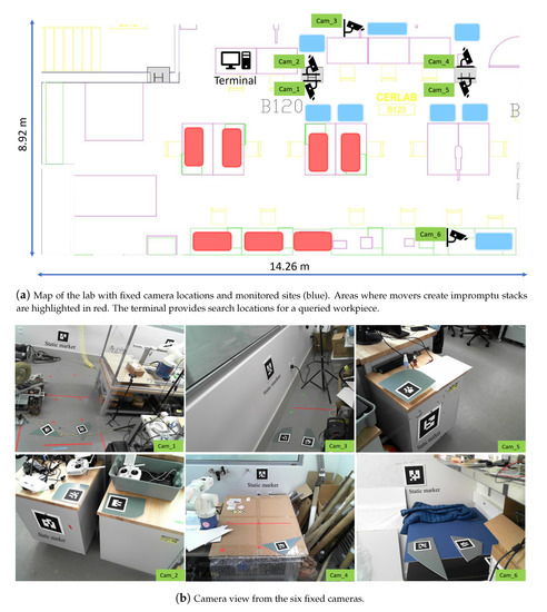
Figure 4.
Workspace scene setup in the lab. (a) Map of our lab with highlighted fixed camera and inventory storage locations. Areas being monitored by the fixed cameras are highlighted in blue whereas areas that are not constantly monitored but represent space where movers could make impromptu stacks are highlighted in red. (b) Images of storage locations containing workpieces (grey) and static markers (white) as viewed by the fixed cameras.
IoT architecture: The objective of the observation module in our approach is to collect information from the viewpoint of movers and from static cameras covering common inventory storage areas. While publishing images through a Robotic Operating System (ROS) [37] network in smaller spaces with strong Wi-Fi, as described in [15], is a solution that provides live updates on inventory movement, this breaks down in larger work sites that have weak or no Wi-Fi signals. A system that can scale and guarantee that observations are not lost despite weak communication channels vastly expands its application and reduces the implementation burden on the environment, making it more attractive for industries to adopt.
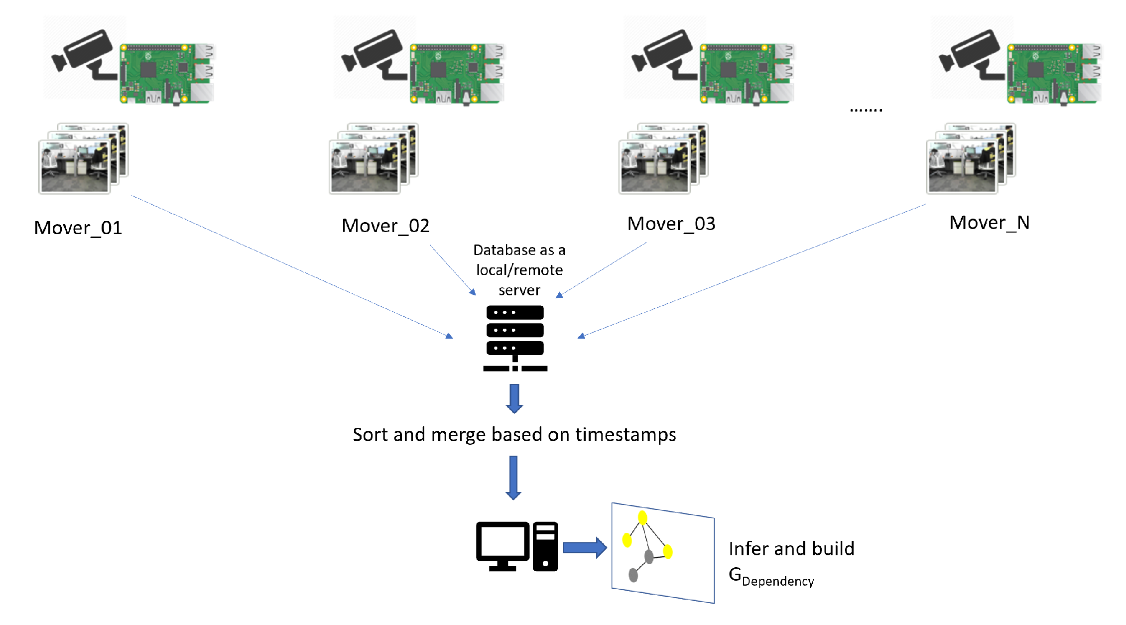
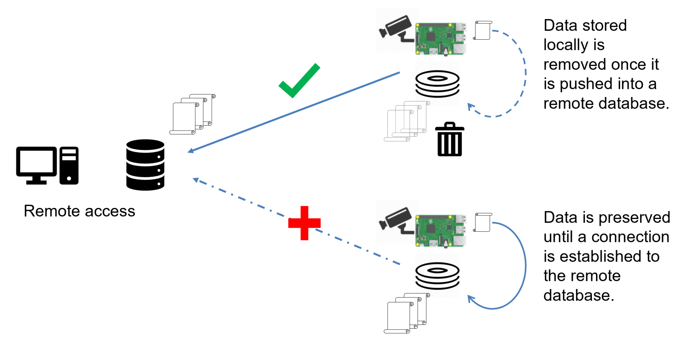
In this work we use an Internet-of-Things (IoT) framework (Figure 5) where the movers and static cameras, with synchronized clocks, push timestamped images onto a remote database. Images from the database can then be pulled and processed by the detection and inference modules, through any terminal that can access the database to estimate possible locations for each workpiece. To make sure that data is not lost when movers are in areas with weak connections, images are stored locally with their timestamps and mover-identifier until a connection can be established (Figure 6). While this system may not be able to provide live updates, the system can run through all observations by the end of the day, when data from all movers are uploaded to a database. This way, data from all movers can be accumulated and processed in offline mode to provide a belief on the location of workpieces for workers on the next day. At the same time, if a strong wireless network for data transfer does exist, updates can be made immediately, and the system can be set to function in an online mode.
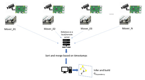
Figure 5.
Scalable IoT-type architecture for information collection. Each mover pushes their observed images onto a database when a connection is available. This architecture allows for images from observers across vast work areas to pool their data, allowing for workpieces to be tracked across the entire scope of the work site.
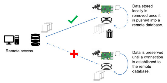
Figure 6.
Offline information collection setup when Wi-Fi is unavailable. For each mover wearing the hardhat as an IoT device, observations as images are transferred to the database immediately when the Wi-Fi signals are strong. However, when a mover is out of range or under poor Wi-Fi coverage, data are locally stored and pushed to the database when a connection can be established. This makes sure that all observations are available at the end of the day when all hardhats are within Wi-Fi range.
3.2. Reasoning Observations
Once observable information is available through the information collection module, possible locations of missing workpieces need to be hypothesized from available information. This is accomplished in the reasoning module that identifies stacking events and builds and evolves such hypotheses for the locations of missing workpieces. Similar approaches to build and evolve hypotheses as beliefs have been successfully employed in localization problems in robotics under ambiguous sensor observations. In this section we give a brief description of the underlying probabilistic concepts and our approach to utilize them for our case.
Theoretical background: Like tracking-by-detection, single-hypothesis approaches in robotic and workpiece localization problems aim to provide a single best-fit solution based on observed data and their correlation to an available model, like geometry [38,39,40]. In cases where a single best-fit cannot be determined due to ambiguity, probabilistic localization approaches preserve ambiguities and maintain multiple relevant hypotheses as distributions and update them as more observations are received [29,41]. In such approaches, a belief of the state of the current system, representative of uncertainty, is maintained. The posterior probability distributions for such hypotheses are calculated based on prior knowledge, observation or sensor characteristics and a model of the object using Bayes rules as described in Equation (1):
where represents the posterior on the object being in some state given sensor observation and some model M of the environment that allows us to calculate the likelihood of the observation and prior . In workpiece localization problems, this model could be geometric information of the workpiece that can provide a fit to observed sensor data. For a series of observations over time, like workpiece locations observed by multiple movers, Equation (1) can be described, using the Bayes rule, at any time-step t as:
Equation (2) is further simplified with the Markov assumption:
which states that older measurements can be ignored once they have been used to update the prior . This also assumes that all observations are independent of each other. Representing as and assuming initial conditions as prior at time Equation (2) can be rewritten as:
where is a normalization factor.
Equation (4) provides the basis to update and maintain multiple hypotheses on the state of the object , as at any time t when a sequence of observations have been made. This is that we have knowledge of a model M that can relate observations to the state of the object. For workpiece or robot localization problems, M is a measurement model that correlates sensor measurements, such as touch, point-clouds or images, with geometric information of the object to compute a fit [30,42].
Now, in our case, since the objective is to search for workpieces that are out of line-of-sight, such geometric correlation models to compute fit are not applicable. Even sensors that do not require a line-of-sight, like RFID, cannot penetrate stacks to read the sensor tags to provide a mode of measurement to work with. Due to these constraints, we propose a reasoning model that represents domain knowledge of human workers to reason possible locations based on available line-of-sight observations. With such a model we might be able to observe events leading up to a workpiece’s occlusion and estimate its possible position. The need to preserve ambiguity here is critical, as for a stacked workpiece, true location will remain latent until it is within line-of-sight to be detected.
As discussed earlier, to have a system that can update beliefs using Equation (4) given an observation of a workpiece k at time t, we need to:
- Measure the fit for it getting stacked with every other workpiece;
- Compute the likelihood of it getting stacked with every other workpiece given the fit;
- Maintain and update the belief of the position of all workpieces given stack likelihoods.
In our work, we represent as the position of workpiece i. The fit for any workpiece k to get stacked with i at any time t is calculated using a graph that monitors linger as fit. For any workpiece k, the probability that k is stacked under i at position at time t representative of stack likelihood, , is calculated from the fit through the event graph. The belief of the system at any time t, , is maintained by the dependency graph at a given time t.
Graph-Based Reasoning Model
We propose a graph-based reasoning model to identify stacking events and propagate its effect in beliefs as described in Equation (4). The entire system consists of three un-directed graphs and one directed graph to observe the workspace, identify the possibility of stacking events between workpieces and infer possible locations at which a missing workpiece might be (Figure 7).

Figure 7.
Linger, event and dependency graphs to calculate stack fit, stack likelihood and overall belief of the positions of workpieces within a workspace, respectively. M represents the reasoning model based on human knowledge of the behavior of stacks and its propagation based on available detections of a workpiece.
3.3. Linger Graph
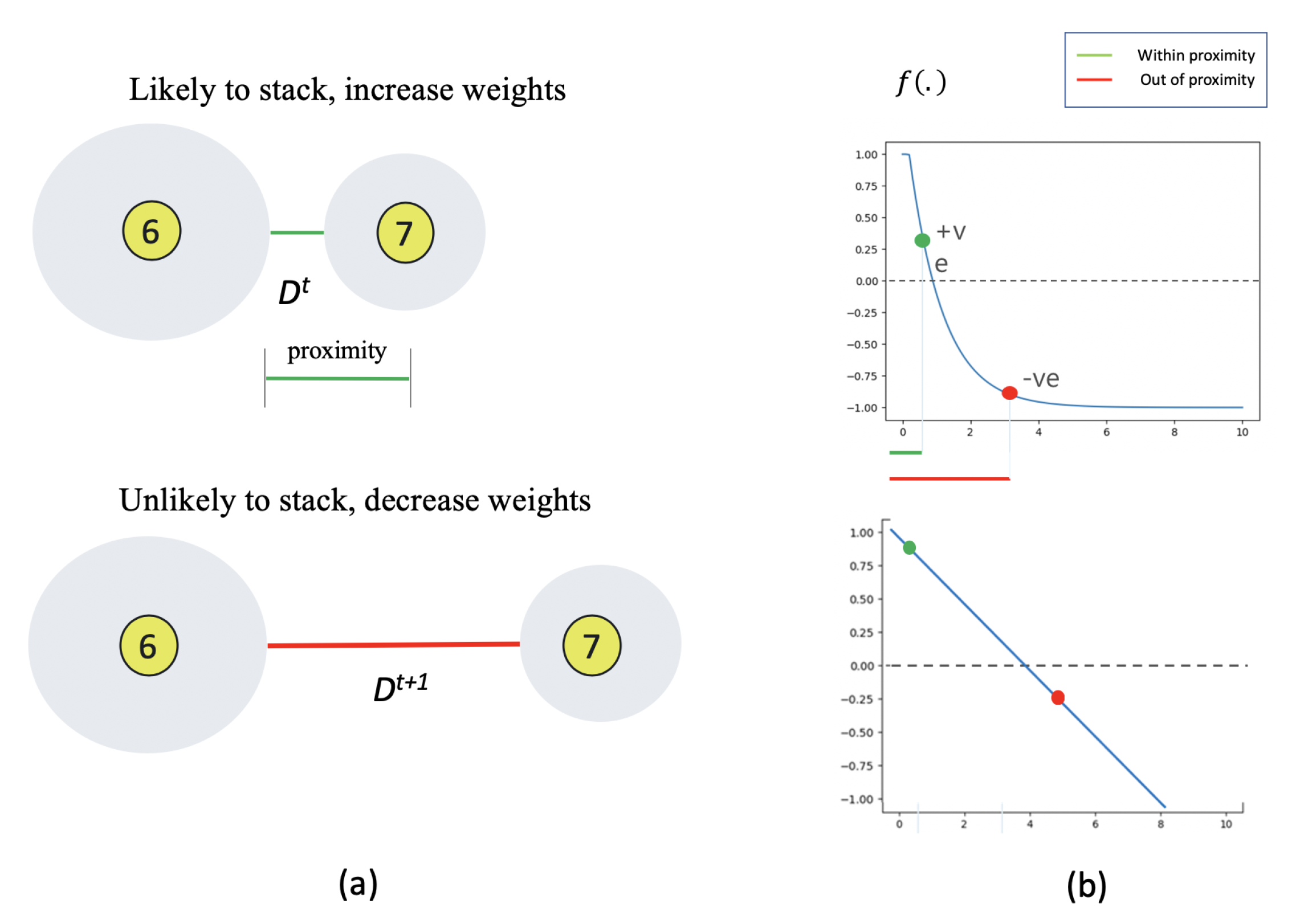
To infer possible stacked locations for a missing workpiece, events that could cause stacking need to be identified. A simple trigger to realize that such a stacking event has taken place is the loss of line-of-sight for a workpiece. When a workpiece disappears, it can be reasoned as an effect of a stacking event. It can also be reasoned, without loss of generality, that if a workpiece disappears, it could only have been stacked with workpieces within a limited neighborhood. To pick such candidates that are within the neighborhood, we need to, at all times, maintain a fit of such possible candidates. This fit of likely candidates is maintained by a linger graph, which weighs candidate workpieces as suspects based on the duration of their lingering near the missing workpiece (Figure 8). Each observed workpiece is represented as a node and the edge weight between any two nodes represents the linger measure. Linger weights are clipped between zero and a max value . The weights are updated for each new observation in time through Equation (6).
where:
| Euclidean distance between workpiece i and j at time t. | |
| Vector representing the most recent available position (xyz) of workpiece i. | |
| Edge weight between workpieces i and j as nodes in the linger graph at time t. | |
| A function, , mapping the distance to positive or negative weights based on a proximity threshold (Figure 8). | |
| Upper limit clip value for linger weight to avoid numerical overflow. |
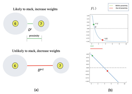
Figure 8.
Calculating pairwise fit for events between workpieces. (a) A representation of cases where linger weights are (top) increased when workpieces are within proximity and (bottom) when workpieces are out of proximity. (b) Examples of to increase and decrease weights based on proximity.
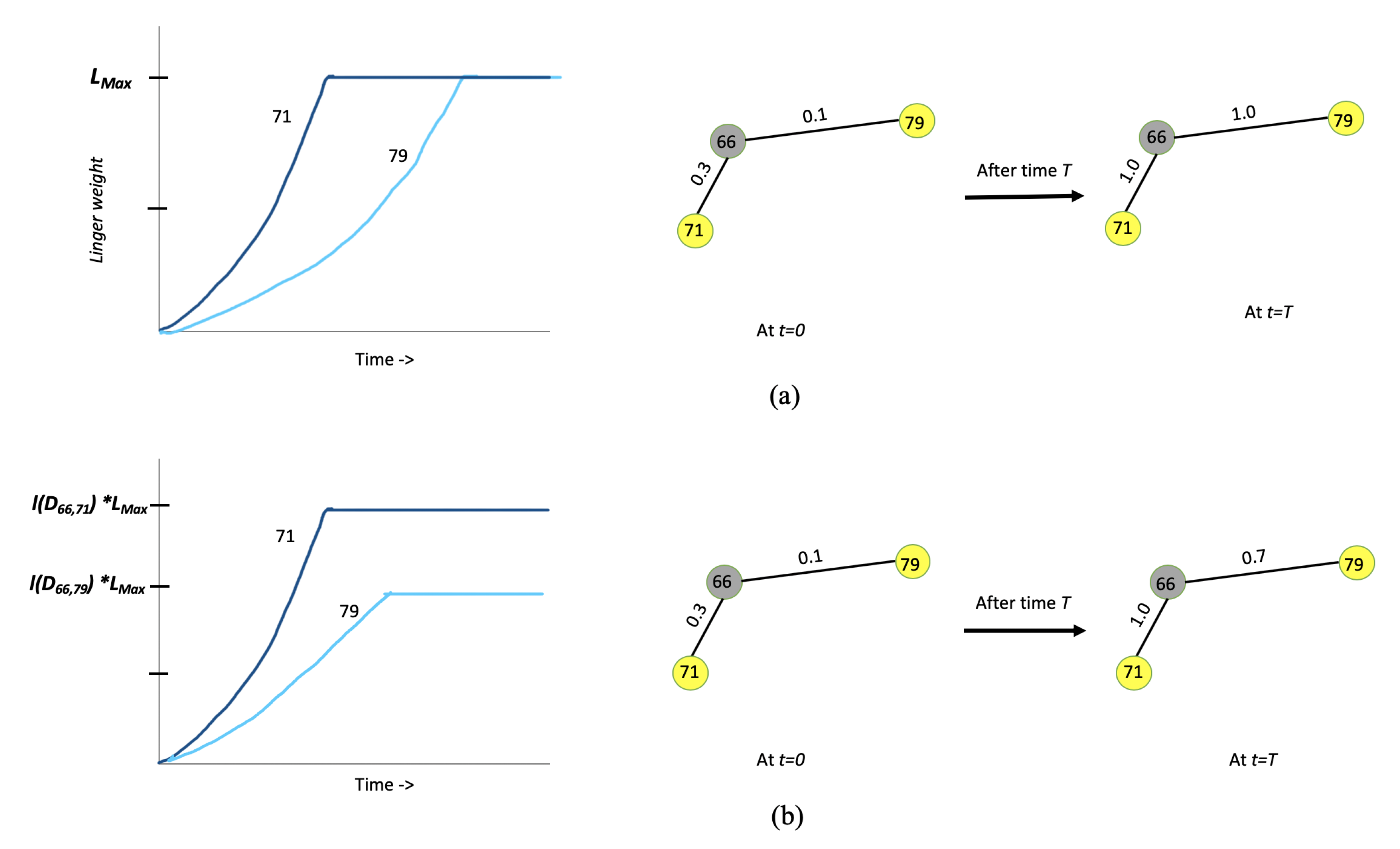
As workpieces tend to stay in positions for long periods of time in unstructured environments, one limitation with accumulating linger weights for edges between workpieces is that all workpieces within proximity, given enough time, reach . While the time it takes for each pair of workpieces to reach is dependent on the distance between them, with larger periods of time, the effect of is lost in the system described in our previous work [15]. This has effects downstream in the rest of the system wherein all workpieces within a neighborhood of a missing workpiece become equally likely stack locations. Further, if they get moved and stacked to other locations, those locations too receive equal weights, which ignores common-sense reasoning that workpieces closest to the missing workpiece should be first in the totem pole for search locations. In this work, we maintain and build on the initial condition of by introducing its effect onto the value of and replacing Equation (6) with Equation (7):
where is any loss function within range that is inversely proportional to . In this way, the system can maintain finer discrimination between workpieces, even within proximity. The effect of using as a factor in calculating linger weights against that of [15] is shown in Figure 9.
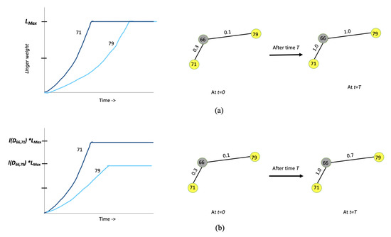
Figure 9.
Previous method (a) cannot differentiate workpieces within proximity after a certain period of time, making them all equally likely stack positions for a missing workpiece. Proposed approach (b) can differentiate most likely stack location even amongst workpieces within a neighborhood.
Apart from being able to model reasoning-based inventory tracking, the pairwise update nature of the graph-based structure allows for simple knowledge insertion as required by the environment. There are several conditions in workpiece movement considered as common knowledge amongst movers that could help in pruning search locations. For example, in shipyards, when two workpieces belong to different projects, even though they might be placed near each other, it is highly unlikely that they would be stacked together by any mover. Another restriction might be certain areas where the workpieces might be very unlikely to be present. Such domain knowledge that might seem obvious to movers can be incorporated into our system by adding appropriate weights to Equation (8) to the edges in the linger graph (Appendix A) that directly affect the fit of observations:
where is based on the constraints dictated by the environment. If there are no such constraints, can be set to 1.0. A value close to 0.0, on the other hand, would transfer the unlikeliness of workpieces i and j getting stacked into the system.
While such additional constraints on workpiece movement were not utilized in our experiments, our proposed system makes it possible to add such common-sense or domain knowledge information without any functional restrictions.
3.4. Event Graph
While the linger graph maintains a measure for each workpiece as a candidate for stacking, it does not identify or react to a stacking event. Identifications and measurements of stacking events are stored and tracked by the event graph in our system. The edges in this graph represent the confidence of the system that a stacking event has taken place between the workpieces involved. Since when a workpiece is visible, it cannot be stacked, non-zero edge weights exist only between workpieces where at least one of them is occluded or missing. Edge weights are calculated based on the linger measure between any two workpieces as described by Equation (9). In this respect, the edges in the event graph represent the pairwise stack likelihood between workpieces. As described in [15] and in Appendix A.2, a cumulative distribution function over an exponential distribution is used as :
where:
| Edge weight between workpieces i and j as nodes in the Event graph at time t. | |
| A squashing function that maps linger weights within a [0,1] interval. |
3.5. Dependency Graph
While the event graph measures pairwise stack likelihood between workpieces, the effect of such events needs to be cumulated to maintain a belief of all possible locations of all the workpieces in a workspace. This update step is similar to the belief update procedure described in Equation (4), where each new observation has an effect on the system’s current belief. Unlike event and linger graphs, where the effect of a new observation of a workpiece is limited to its immediate spatial neighborhoods, the dependency graph maintains and updates all possible hypotheses involving the workpiece. As a result, for any new observation of a workpiece, all nodes reachable from it in the dependency graph are affected.
Since the dependency graph represents the belief, as an initial condition, all visible workpieces are assumed to be independently placed with no stacks and hence no edges. As more observations and stack events are identified, edges in the dependency graph are populated adding direct edges based on piece-wise events and indirect edges based on all connected nodes to the workpieces involved in the event. While the steps involved in updating the dependency graph are described in detail in our previous work [15], there, the order of stack formation was not considered, resulting in excess edges that can further be pruned.
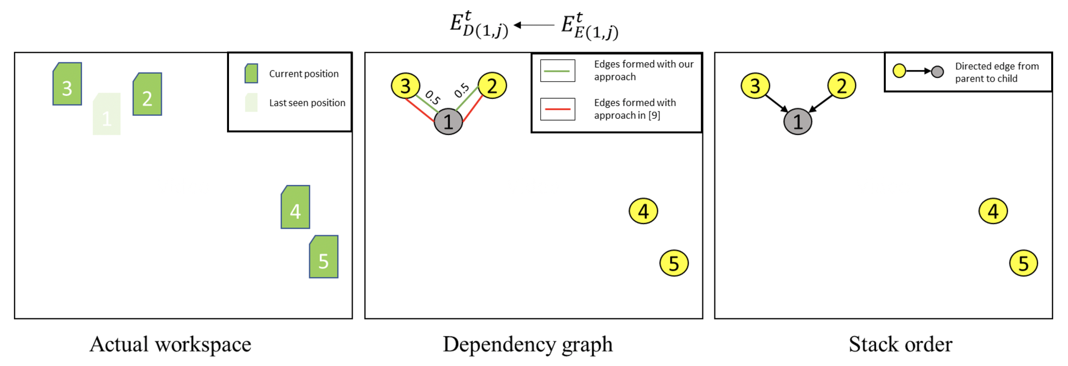
In this work, stack order is also tracked in the memory of the system as a separate directed graph. This information on the order of stacking allows us to further limit search locations compared to the previous system without losing any feasible locations. By preserving the order of stacking through a directional graph, indirect stack relations are added to the dependency graph based on the ancestors of a node, as opposed to all reachable members (Appendix A.3). We highlight the benefit of pruning with a simple scene shown in Figure 10. Here, since workpiece 1 is no longer visible, the dependency graph pulls possible events that could have taken place. This creates edges and , as workpieces 2 and 3 were nearby. At the same time, in the ordered graph that tracks stack order, workpieces 2 and 3 are identified as the ancestors of workpiece 1, as it could be stacked under either one.
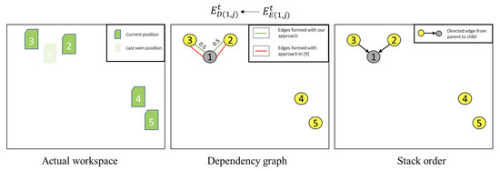
Figure 10.
When workpiece 1 becomes occluded near workpieces 2 and 3, stack order sets workpieces 2 and 3 as possible parent nodes for workpiece 1. This represents the case where workpiece 1 could be stacked under 2 or 3.
Now, if workpiece 2 moves nearer to workpiece 4 (Figure 11), no new edges are formed as there are no visibility changes or events to update the belief of the system. However, the linger graph gets updated constantly for every new observation. This creates a strong fit for a stacking event between workpieces 2 and 4. There are no changes in the edges of the stack order graph either, as no new stacks have been recognized by the system. Up to this point, the belief of our system is identical to that described in [15].

Figure 11.
The dependency graph state in our current approach and previous approach is exactly the same up to this scene.
However, when workpiece 2 gets stacked under workpiece 4 (Figure 12), the visibility of workpiece 2 changes to occluded, triggering an event. The event graph queries the linger graph to find the workpieces that have non-zero fit values with workpiece 2 to build edges that represent the likelihood of stacking. This creates edge in the event and dependency graphs. Note that an edge is also formed between workpieces 2 and 3 in the previous method though there is no reason to believe that workpiece 2 could be stacked with 3. This is because edges are based on reachable nodes from workpiece 2 in an un-directed graph in our previous approach. However, if the order of stacking is stored in a directed graph, we can populate the required indirect relations between workpieces by replacing all reachable nodes with all ancestors of workpiece 2. This avoids unnecessary edge formation between workpieces 2 and 3. While in this scenario our approach prunes off just a single edge, as more events are observed, using stack order can avoid all further connections between workpiece 2 and all stack relations that workpiece 3 might encounter.

Figure 12.
Since the previous approach only used un-directed graphs and ignored stack order to build dependencies, an edge representing the possibility of workpiece 2 being stacked with 3 is spawned though it is an unnecessary search location. Using stack order, this can be avoided in our approach by limiting indirect edges to all ancestors and sibling nodes, as workpiece 3 is not an ancestor of 2. Since workpiece 4 is still an ancestor of 1, and since workpiece 1 could possibly be under 4, this indirect edge (blue) as a search location is still valid.
Inference from Local hardhat Observations
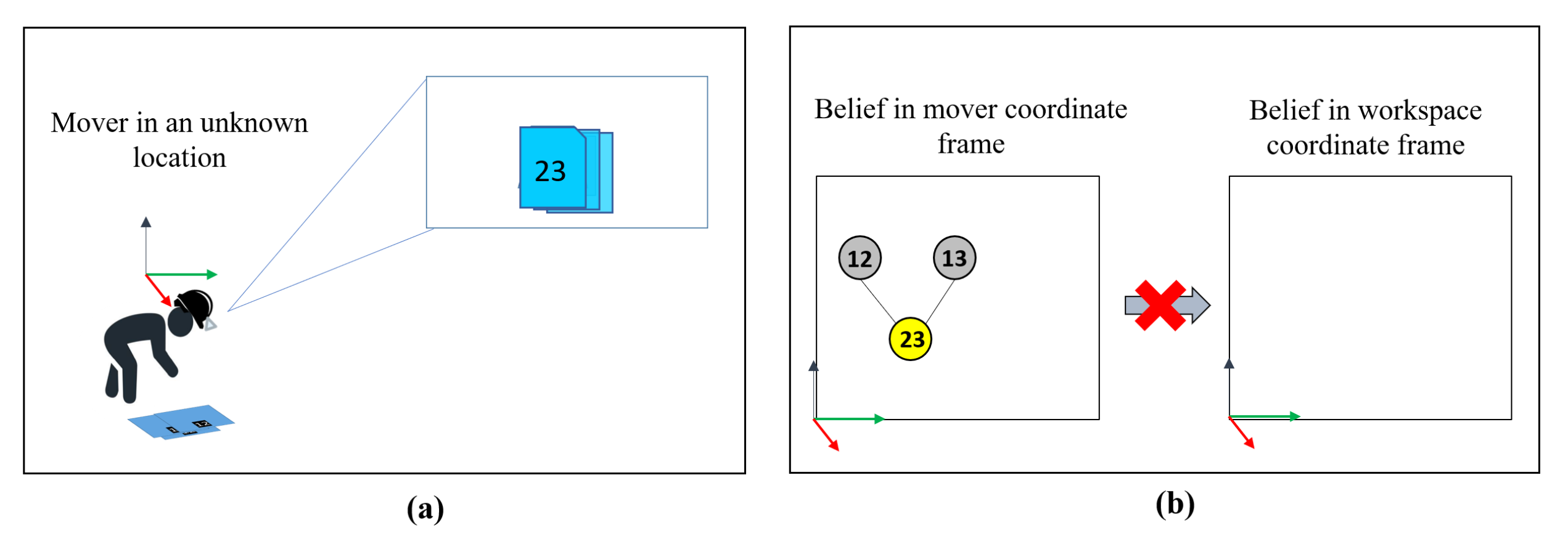
One of the critical limitations with the system described in our previous work [15] is that for any observation of a workpiece to even be considered as an event, the location of the workpiece with respect to the workspace needs to be known. Since the observation is processed based on the possibility of its effect on other workpieces present within the workspace, lack of location information leads to that observation being discarded. However, this also means that other relevant information that was available within this observation is discarded. To highlight our reference to other relevant information, consider the case shown in (Figure 13) where a worker whose position is unknown stacks workpieces 12 and 13, with workpiece 23 ending up on top of the stack. Since the worker’s position with respect to the workspace is unknown, and the position of the workpieces observed by the worker is also unknown. When workpiece 23 is finally observed by a mover whose world position is established, then it gets registered in the graphs as a single workpiece.
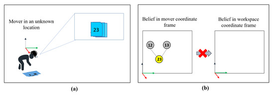
Figure 13.
Extracting critical information from local observations. (a) When a mover observes workpieces and stacks them while his/her position is unknown, dependencies between workpieces is locally extracted. (b) Since the positions of the worker and the workpieces are unknown, this information is not reflected in the dependency graph for the workspace.
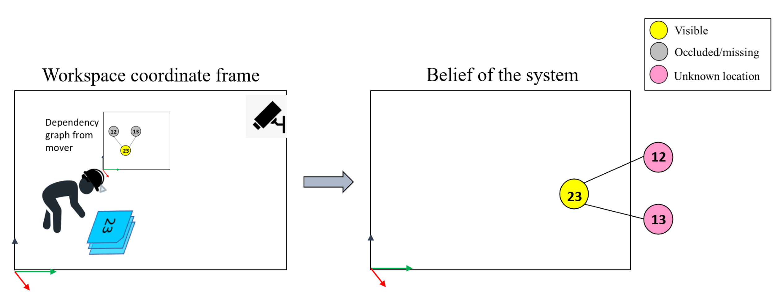
In the above case, there is enough evidence observed from the worker to realize that workpieces 13 and 12 were stacked under workpiece 23, though we cannot establish where any of the workpieces were at that time of stacking (Figure 13). The critical information that needs to be preserved is that events that related workpieces 13 and 12 with 23 were observed locally by the mover. This information is useful even if we cannot establish where such a stack was formed. As shown in Figure 14, later when workpiece 23 is observed, with available evidence, we can hypothesize that workpieces 13 and 12 could still be stacked with 23 given no information to contradict it. In such cases, the last-seen positions of the locally observed workpieces are unknown but their likely positions as being stacked under other observed workpieces is presented as search locations.
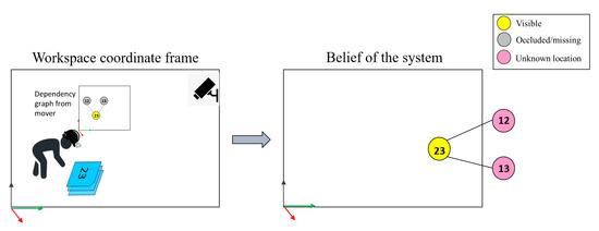
Figure 14.
Transferring locally observed stack information. When a mover observes the stacked workpieces when his/her own position with respect to the workspace is known, workpiece 23, the only visible member of the stack, is registered in the dependency graph. Additionally, since the earlier local dependency graph by the mover established that workpieces 12 and 13 were associated with 23, this information gets transferred to the workspace though they were never directly observed within the workspace.
The situation depicted by Figure 13 is quite common when multiple movers make decisions to move, stack or split stacks based on their immediate requirements. While it may not be possible to predict what decisions are made and why, it is possible to record and reason the effect of such decisions from the viewpoint of the mover even if the mover’s location cannot be determined.
One way to extract and use local observations is to run multiple instances of the system under different scopes. A primary dependency graph, , covers the scope of the workspace and is run as discussed in the previous sections. Whenever a mover, say , observes workpieces whose position cannot be determined with respect to the workspace, a temporary graph is spawned. This graph extracts dependencies within the field of view of assuming the camera origin to be the local workspace origin (Figure 13). If interactions were observed, creating edges in , then these edges, their weights and their associated nodes representing workpieces, are added to without any location information. In this way, local knowledge of stacks observed by any mover gets transferred. Since these workpieces cannot be categorized as visible or occluded, they exist in an unknown-location state within the system. However, the edges hold critical stacking information as possible location of workpieces. This can be utilized in case any of the locally observed workpieces later become visible, as shown in Figure 14.
One challenge that needs to be addressed here is that since we cannot determine the pose or position of the mover, all observations are mapped into the same local coordinate system spanned by the mover’s camera. This leads to workpieces located at different positions in the workspace being mapped to overlapped positions within the view of the mover’s camera coordinate system. To overcome this issue, the graph of any mover gets reset whenever there are no workpieces within view. All dependencies as edges are transferred to the primary dependency graph before clearing the local graph nodes and edges. This makes sure that when a worker moves away from or changes their view, a new instance for local observations are spawned for the new local workspace.
Since movers make a variety of impromptu decisions to grab and stack workpieces, extracting such decisions and their effect is critical to build a tight belief on the location of workpieces. While it may not be possible to densely populate a workspace with fixed cameras to capture all events, using hardhats to extract events through the viewpoint of movers provides far more coverage of all critical events right at the source. The critical nature of extracting such local stack events from moves is highlighted in our experiments in the next section.
4. Experiments
As discussed earlier, the purpose of our proposed system is to reduce effort and time spent in searching for workpieces without adding any additional cognitive burden on the movers during workpiece displacements, accidental or otherwise. One way to evaluate the system would be to compare inventory pull costs with our proposed approach against current industry practices.
However, in our literature review, we could not find standard databases or test procedures to measure the performance of generic inventory tracking systems. Apart from lack of databases, standard simulation environments and tools to model complex workpiece movements and actor interactions, such as an Actor Based Model (ABM) environment, while of interest, are still in early stages of development [43,44]. Previous work investigating poor pull times [4,8,10] in the construction industry have compared the cost of pulling inventory when their position is known against cases where they have been misplaced without any information to guide a search. Since such observations have been the basis to investigate and show that excessive pull costs are the result of a lack of efficient inventory tracking systems, we use a similar approach to evaluate our proposed system within the confines of our lab (Figure 4). To show that such a system can be deployed in a real-world environment, we have also conducted simple experiments in a shipyard at Tsuneishi under real-world conditions such as lighting, workpieces and untrained movers (Figure 3). The following sections discuss the results of experiments conducted both in our lab and at the shipyard.
4.1. In-Lab Experiments
In order to evaluate our system, we designed a workspace in our lab similar to unstructured storage spots used in the construction or shipbuilding industries for convenient and impromptu storage of workpieces. Our workspace setup consists of six fixed cameras, connected to four battery-powered Raspberry Pis, which monitor areas representing storage locations within the workspace. Note that while such storage locations are marked for monitoring by fixed cameras, there are no explicit rules or policies to drive incoming and outgoing inventory. This setup represents a workspace within which workpieces are stacked and displaced independently by movers wearing camera-mounted hardhats (Figure 2). As discussed in Section 3.5, the hardhats capture critical events involving workpieces that might have taken place away from the view of the fixed cameras but within the field of view of the mover. While the span of our experimental space might be much smaller than a typical environment in a construction or shipbuilding environment, with 25 different stacks populated throughout the space, search for a missing workpiece, given no further information, requires a lot of effort (Table 1).

Table 1.
Cost of search in terms of number of workpieces to be visited and distance covered to find workpiece 66 displaced to various locations P1–P6. Least number of workpieces to be visited and the least distance covered during the search are highlighted in green.
Experiment design: Evaluation of our proposed approach was conducted through a sequence of three staggered experiment phases set up to emulate workpiece population, stacking and displacement in an unstructured storage environment (Figure 4). During the experiment, workpiece 66 was displaced across the workspace by the movers. The performance of our system was based on the number of locations and distance a mover covers to find workpiece 66 using its suggested search locations. In the first phase of the experiment, the workspace was populated with 25 workpieces by two independent movers. Locations of the workpieces were predetermined for the repeatability of experiments and ground truth evaluation of our system. For the system, observations older than two seconds are considered occluded. The value for , described in earlier sections, was set to 100. The function to limit (Figure 9), discussed in Section 3.3, was defined as a linear hinge-loss function that decreases from 1.0 to 0.0 for distances, , ranging from 0.0 to 0.5 m. The separation penalty that penalizes indirect stacking relations to dampen the effect of indirect stack events, was set to 0.5. A value of 1.0 for translates to all events, no matter how indirect, to have equal significance during a search. On the other extreme, a value of 0.0 for translates to no event being considered for search, reducing the system to present the last-seen position as the only search location. The effect and need for is explained in detail in [15]. Experiments were conducted under the same values for common parameters between the current and previous approach.
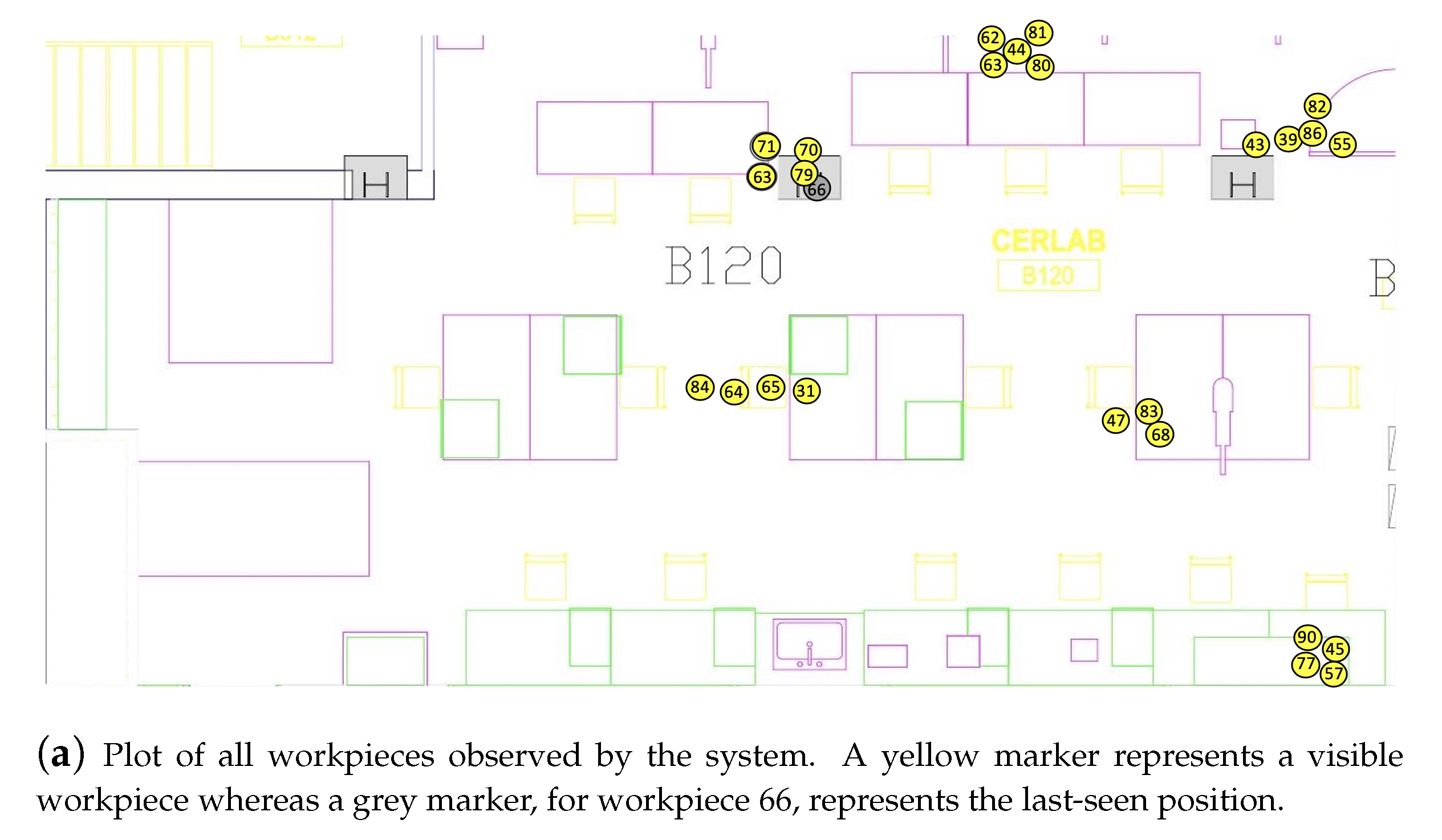
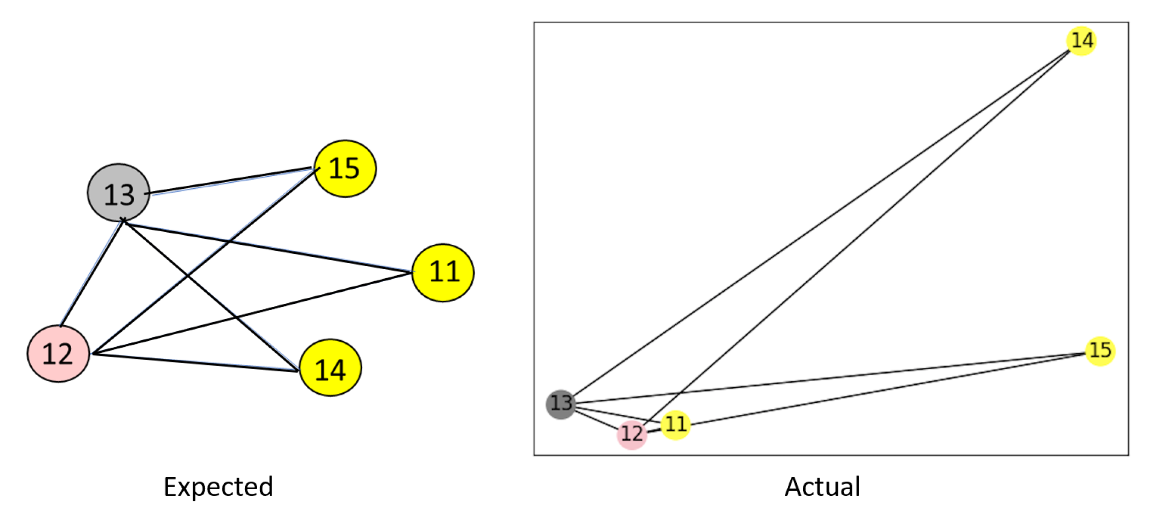
Phase 1: Since the goal of our proposed approach is to passively collect and present workpiece location information to the rest of the movers, observed positions of workpieces were plotted on a map and checked against the ground truth location of each workpiece. Figure 15 shows the plot of all workpieces that were observed by our system. This experimental evaluation serves to qualify the information collection using AR markers for our system. While this experiment is simple with no stacking of workpieces, a lookup map of workpiece locations provides a CPS of the current state of the workpieces within the workspace. With such a system, workpiece placement decisions made by individual movers get conveyed to the rest of the workforce without adding any burden to the mover. While AR markers detection is used as the mode of information collection in our system, any other mode of detection that provides the workpiece ID and its location can be used as an alternative. This experiment, at the least, qualifies the sanity of the information collection module of our system.
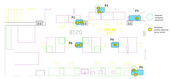
Figure 15.
Map of the workspace with observed workpieces after the first phase of the experiment. Expected (green) and observed (yellow) positions by our system plotted on a map. This information collection makes locations of workpieces available to the entire workforce and allows for fast pull times without need for manual logging.
Phase 2: For the second phase of the experiment, more workpieces were introduced into the workspace wherein stacks were created to store new workpieces under limited storage space. This is a common mode of storage in unstructured environments, which presents challenges for direct visual searching due to clutter and lack of line-of-sight to the workpiece. As discussed earlier, such stacking also introduces challenges for the RFID-based mode of detection, as the interrogation signal cannot penetrate thick stacks. Apart from penetration issues, passive RFID tags, when closely stacked, introduce noise and are difficult to untangle by the reader [27]. In such stacked scenarios, our vision-based information collection system faces the same challenges and cannot extract any more information once a workpiece is occluded. The inference module of our system, described in Section 3.2, however, can hypothesize the positions of workpieces that are out of line-of-sight based on previously identified relevant events (Figure 16). While our proposed approach presents the possible location of any workpiece, visible or occluded, based on surrounding events, one could argue that a system that presents the last known position of a workpiece would produce the same results, provided the stack itself is not moved or disturbed. This condition was further perturbed in the next phase of our experiment.
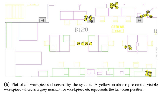
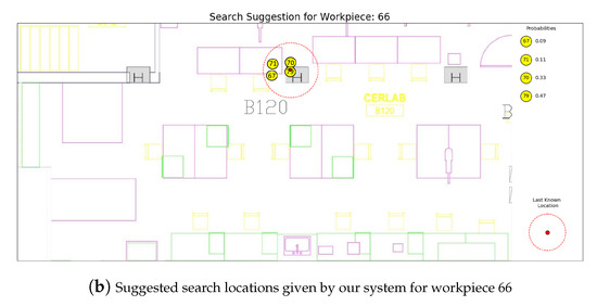
Figure 16.
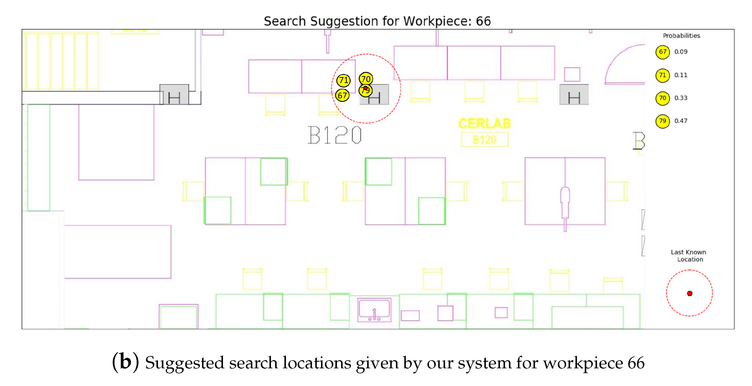
Snapshot of the workspace and belief of our system after the second phase of the experiment. (a) Current location of all workpieces plotted by our system. Locations of recently observed workpieces (within a duration of 3.0 seconds) are highlighted in yellow, whereas workpieces that are deemed missing or occluded are highlighted in grey. (b) A query for the missing workpiece, workpiece 66, produces a plot of likely locations and their probabilities in finding workpiece 66 stacked under there. Workpiece 79 gets the highest confidence due to its proximity to 66, making it the first location to search.
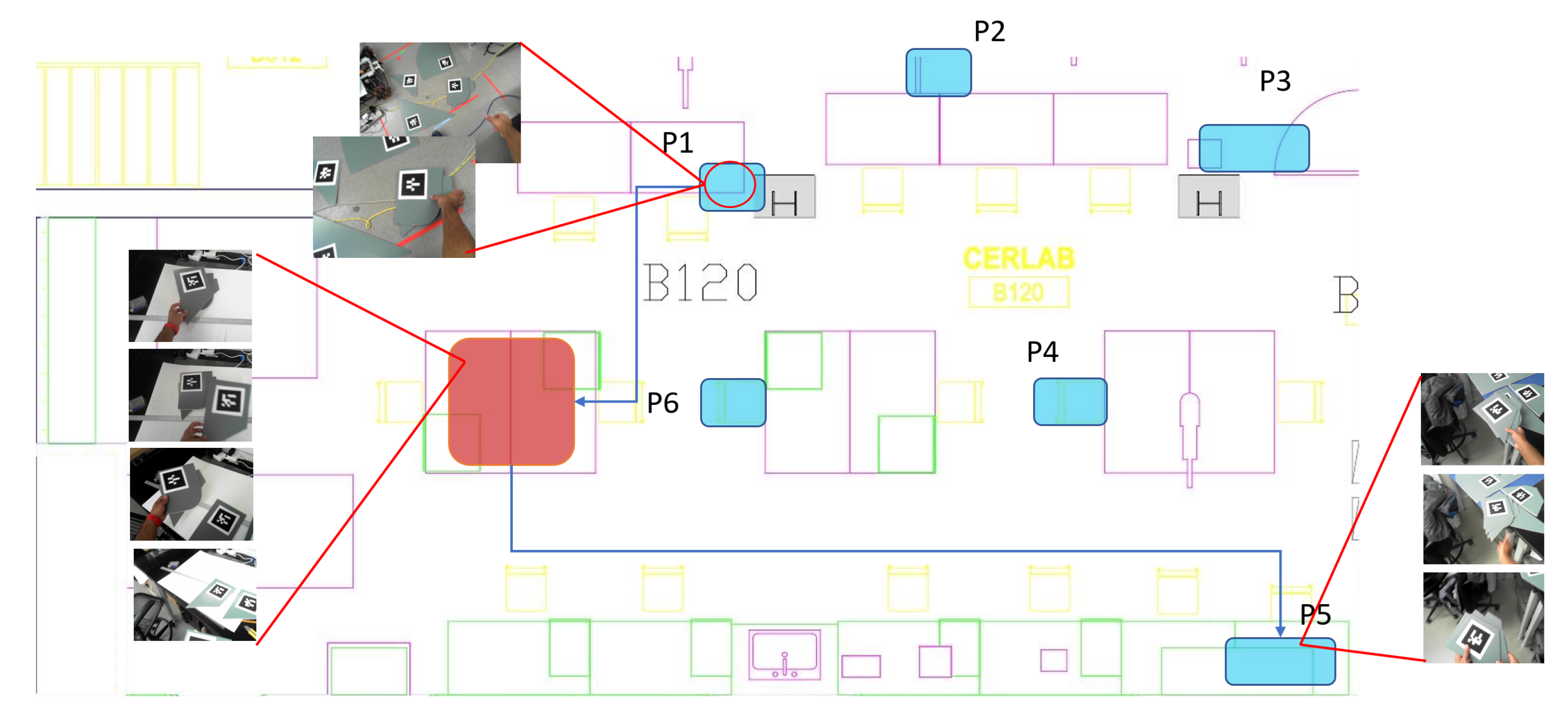
Phase 3: The third and final phase of our experiment covered the cases that are most challenging and highlights the advantages of our approach. This phase of the experiment represents cases where a mover stacks multiple stacks together and displaces the whole stack to other locations either accidentally or intentionally. Either way, such decisions of repeated stacking and displacement are not logged or taken account of in current workspaces to inform the rest of the workforce of the updated position of all the members of the stack [4]. Moreover, while making such impromptu decisions, the movers themselves are not aware of all the members of the stack they just displaced and cannot afford the time to make note of such information at every event. Such gaps in knowledge make it quite difficult for the worker searching for one of the members of the stack when it is no longer at its last seen position, rendering the workpiece lost as far as the shop-floor is concerned. With no further information to guide his/her search, a worker usually resorts to exhaustive time-consuming searches or just re-manufactures the workpiece. This scenario (Figure 17) is reproduced in our experimental workspace by:
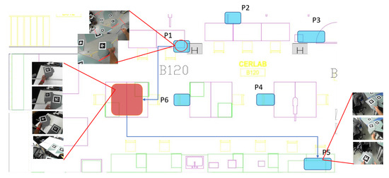
Figure 17.
Events, viewed by the hardhat camera of a mover, during the third and final phase of the experiment. The view at location P1 shows a mover picking up the stack with workpieces 79 and 66. The view at a random location (red) away from monitored areas shows the mover stacking workpieces 33 and 35 on the existing stack. The view at location P5 shows the mover placing the new stack with workpieces 66, 79, 33 and 35 on top of workpiece 77.
- Having a mover remove the stack containing workpieces 66 and 79.
- Stacking workpieces 33 and 35 on top of this stack, away from fixed camera view in areas highlighted in red on the map (Figure 4).
- Placing the new stack, with workpiece 35 at the top of the stack, on top of another stack within the workspace.
These actions are repeated multiple times by movers to lose workpiece 66 throughout all storage locations, P1–P6, within our workspace. The entire experiment was conducted across a span of two weeks in total to present a case as close to the real world as possible where movers interact with workpieces over a longer duration of time.
Evaluation criteria: Once the third phase of the experiment was completed by a mover, the entire workspace was reset to its original state defined in the first phase of the experiment. Table 2 shows the suggested workpieces to look under, as search locations, for every location P1–P6 that workpiece 66 was displaced to. Table 1 shows the cost, in workpiece visits and steps, that would be incurred under four different cases where a worker is given:

Table 2.
Totem pole and confidence of search locations for each experiment where workpiece 66 is moved to each of the six locations P1 to P6. The true location of workpiece 66 is highlighted in green. The locations are listed in the order of search locations along with their probability values as suggested by our system for each displacement.
- Last-seen information: This represents the case when a worker is aware of the original location where workpiece 66 was placed in the first phase of the experiment but has no information of further events that have taken place.
- Information using previous system [15]: This provides search locations based on events observed by fixed cameras monitoring storage locations. Local events observed by the workers away from fixed camera view are still lost.
- Information from our proposed approach: In this case the worker solicits our system to provide search locations for workpiece 66.
As mentioned earlier, the objective of the proposed approach is to reduce the effort and cost of searching for workpieces that have been displaced by multiple stakeholders within the workspace. The evaluation criteria for inventory pull are based on the number of workpieces a worker would have to visit and the distance covered in such visits before finding workpiece 66. Since workpiece 66 is not directly visible, the complete search space spans the location of every other workpiece within our workspace. When a totem pole of locations to visit is available, the number of workpieces a worker would have to visit is based on the position of the true location within this list. When no totem pole exists, all workpieces within a location are considered equally likely. In this case, the expected number of workpieces one would have to visit can be shown to be , where N is the number of equally likely choices available. If workpiece 66 was not found in a location, a worker moves on to the next location based on the suggested search location or optimal search path for continued search. Distance covered is based on the distance a worker has to travel from location P1, as that is the last seen position for workpiece 66 and would be the first location a worker would start the search from. Our system was evaluated against our previous approach and search based on optimal search paths to cover all locations. The optimal path based on distance to visit all workpiece locations in the case of our workspace is to sequentially move from P1 to P6.
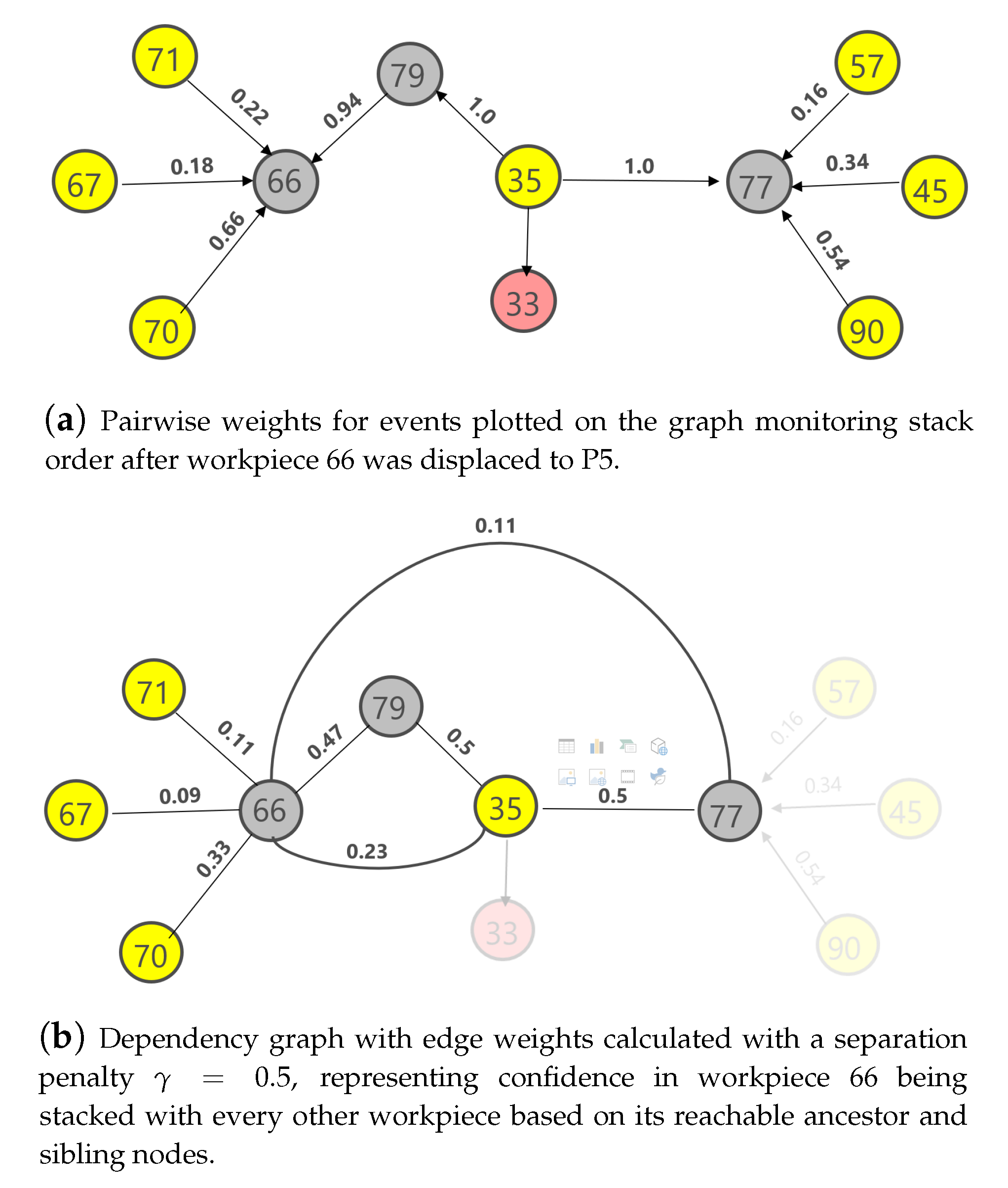
Discussion: As seen from Table 1, the average number of workpieces to be visited by our proposed approach was 80% lower than manual uninformed searches and the previous approach. The average distance covered by a worker in searching for workpiece 66 was also lower by 60%. One critical observation to emphasize here is that the search cost of our proposed approach is not affected by workpieces that never interacted with it. While a manual search cost is directly influenced by the number of storage locations between workpiece 66’s last seen position and final position, our objective is to limit the search based only on events of interaction involving workpiece 66. This can be seen in the snapshot, as shown in Figure 18, of the event graph edge weights overlaid on the stack order graph and the dependency graph within our system that has captured the chain of events involving workpiece 66 when it was displaced to location P5. This highlights every possible workpiece that workpiece 66 might be stacked under along the way when it was moved to P5.
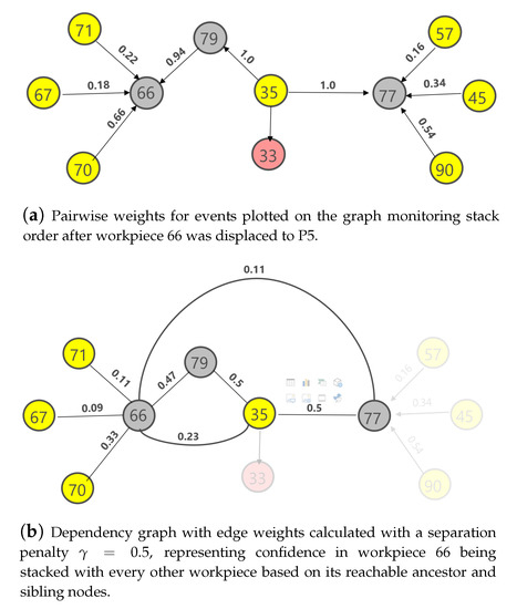
Figure 18.
Underlying graphs in our system calculating beliefs after displacement of workpiece 66 during the experiment. (a) A snapshot of the event weights and stack order of events that workpiece 66 could have encountered, as a directed graph, in the experiment run that displaced workpiece 66 to location P5. (b) The workpieces and their corresponding probability as search locations for the missing workpiece 66. Note that since workpiece 33’s location is unknown, it is not suggested as a search location. Additionally, workpieces 57, 45 and 90 are not considered, as there are no reasonable events connecting them to the directed graph either as an ancestor or a sibling.
Capturing all possible interactions of the workpiece makes the search strategy of the proposed system independent of workpieces that could not have interacted with the missing workpiece. In the absence of this information, the search space for a missing workpiece expands to all locations within the workspace, requiring much more effort and time to search. While the objective of our previous approach in [15] is the same, as shown in Table 1, failure to capture events defaults the cost to manual uninformed search. Since the previous approach could not account for events taking place locally within the field of view of movers, critical information that could have helped in the search was discarded. The significance of such local observations from the point of view of movers that cause stacking events is highlighted in the experiments conducted in the lab.
4.2. Real-World Evaluation
To test the system within a real-world environment outside of our lab, we conducted multiple experiments at the Tsuneishi shipyard. The goal of these experiments was to gauge the ability of our proposed system to collect local events and build the expected dependencies between workpieces from the view of movers using realistic workpieces, and under operation of workers who have never used the system (Figure 3). Since the objective here is to see if we can extract critical events and dependencies between workpieces, event weights are not highlighted as no search is being conducted and have no bearing in this exercise.
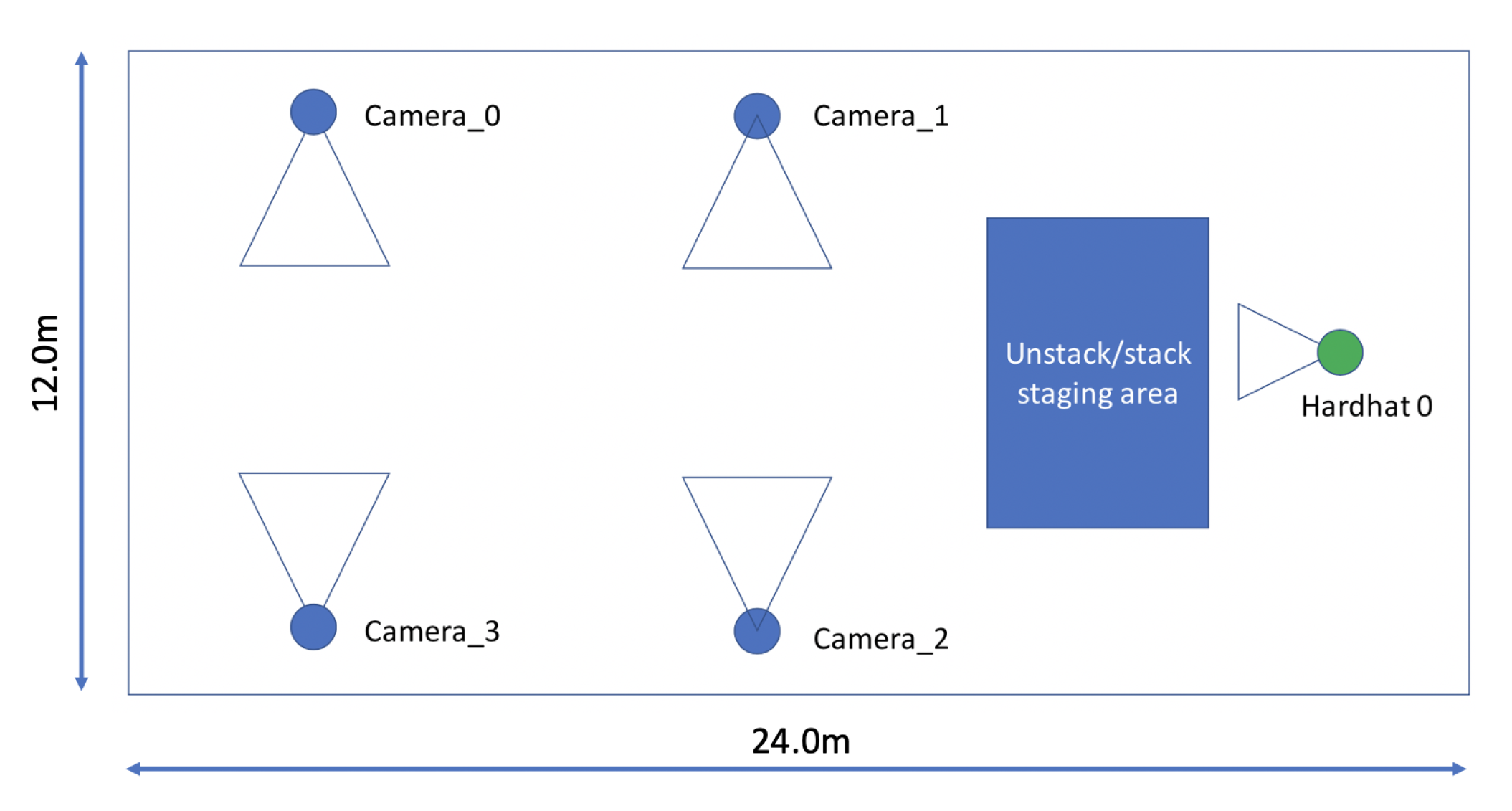
In this experimental space, we were able evaluate our system under real-world conditions with poor lighting, sparse Wi-Fi and mover behavior. Our setup consisted of one hardhat camera and four fixed cameras, two of which were hardwired into the main computer, and two others connected to battery-powered Raspberry-Pis (Figure 19).

Figure 19.
Experimental setup and layout of testing space in the shipyard environment.
The experiment was broken down into three sub-experiments. The first portion of the experiment was to introduce workpieces within the staging area and perform a stacking operation under observation of the hardhat but before entering the fixed camera views. This was done by:
- Having the first mover bring workpieces 11, 12 and 13 into the staging area.
- Stacking them all together and forming the stack (11, 12, 13).
- Moving the stack (11, 12, 13) into view of Camera 1.
The result of this sub-experiment would have connections between workpieces 11, 12 and 13 because they were stacked together within view of the mover’s hardhat camera. Workpieces 11 and 12 will not have absolute locations and will be marked as so (pink node) in the graph. However, since workpiece 13 is directly visible, its position is known and marked as visible (yellow node). Figure 20 shows the expected dependency graph, showing that the stack relation between workpieces matches the actual relation as a graph produced by our system.
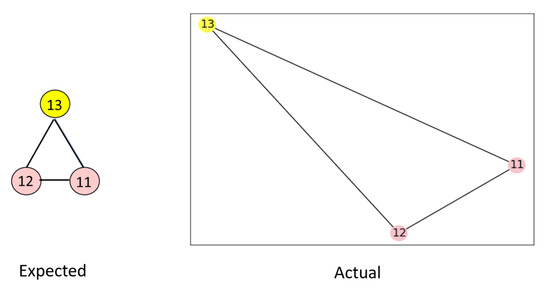
Figure 20.
Workpiece relations, as a graph, for the first experiment. The expected relation between workpieces from the scripted experiment (left) matches the relational graph published by our system (right).
Another mover was then asked to perform the second sub-experiment, where they combined two separate stacks within view of a fixed camera. This was done by:
- Having a new mover place workpieces 14 and 15 into the staging area.
- Stacking workpiece 15 on top of 14, forming the stack (14, 15).
- Moving the stack (14, 15) into the view of Camera 1, and placing it on top of the previous stack (11, 12, 13).
- Another mover comes and moves the whole stack (11, 12, 13, 14, 15) into the staging area.
The resulting graph for this sub-experiment would be an interconnection between all of the workpieces because the two stacks were joined into one (Figure 21).
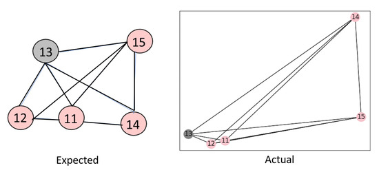
Figure 21.
Workpiece relations for the second experiment. Expected fully connected relation between workpieces (left) and the relational graph published by our system (right), which was able to infer the same relation.
This new worker who came into the last sub-experiment was then asked to continue by:
- Shuffling the stack (11, 12, 13, 14, 15), removing workpiece 11 during the process.
- Splitting the remaining shuffled stack (12, 13, 14, 15) into stacks (12, 14) and (13, 15).
- Placing workpiece 11 in view of Camera 1.
- Placing the stack (12, 14) in view of Camera 0.
- Placing the stack (13, 15) in view of Camera 4.
The graph corresponding to this sequence of events shows that workpieces 11, 14 and 15 can all be seen and that their absolute locations are known. Workpieces 12 and 13 are not on the top of their stacks so they are not seen. The difference between workpieces 12 and 13 is that workpiece 12 was seen during the shuffling and re-stacking in the staging area, while workpiece 13 was never seen. Since the system cannot determine the order of shuffling or the members for the split stacks, workpiece 12 and 13 could be under any of the three visible workpieces 15, 11 and 14 (Figure 22).

Figure 22.
Workpiece relation for the third stage of the experiment. Expected relation between workpieces after the stack was shuffled and split (left), which matches the output of our system (right).
Discussion: While the above experiments are much shorter and simpler than the experiments conducted in our lab, they serve to highlight the robustness and practicality of our proposed approach for industrial applications. The workers that participated in the experiments required no specific training or modifications to their regular behavior to utilize the system successfully. These experiments show that our proposed system can extract critical events regarding workpiece movement and stacking without adding any additional burden to the workers.
5. Conclusions and Future Work
Current proposed solutions for inventory tracking in unstructured environments focus on conditioning and preparing the environment to adapt to mature track-by-detection technologies like RFID. However, the gap between industries with unstructured storage environments and the technology for such adaptation is still challenging. In this work we proposed alternatives to the track-by-detection approach to improve over current practices of searching for lost workpieces without guidance. From experiments, we have shown that even with a simple mode of detection that has severe limitations with occlusions from stacking, reasoning events leading up to occlusion can significantly help narrow search locations. We have also shown that the proposed graph-based tiered approach of reasoning allows for easy additional knowledge insertion, if available, to further prune search locations. For application in adverse environments with sparse Wi-Fi, we have proposed an IoT architecture that enables the system to collect and process information in both offline and online modes of operation.
While the proposed approach expands information collection over our previous approach to better estimate workpiece locations, the entire system is still dependent on observations and detection to build its belief. As shown in the experiments, extracting events is extremely critical, and missing an event would default the system to unguided search thereafter. Currently, our approach uses a single mode of information collection relying on AR markers and vision. However, the system can be further expanded if it can assimilate observations from multiple modes of detection spanning RFID, GPS, vision etc. since they also relay similar position and identity information.
With regards to the reasoning algorithm, currently, observation of a completely empty space that was previously suspected to be the location of a missing workpiece has no effect on the system’s belief. By contrast, in the real world, when a worker visits a location that has no workpieces in it, this information does have an effect on the belief for every other workpiece that was previously suspected to be present there. In our current algorithm, while we can detect the presence of a workpiece with absolute certainty, we are not able to infer or translate the effect of absence of a workpiece at a location. We are currently exploring methods to identify and differentiate an obscured workspace in an image against an empty location that has no workpieces present.
Another observation on the behavior of the system is that while it acts as an information sink, uncertainty or entropy of proposed search locations will tend to increase with more observed events involving a workpiece. Since the system actively maintains multiple hypotheses on the location of a missing workpiece, unless the workpiece is later directly observed, the system cannot inherently take action to prune the search locations. A further expansion of this approach would be to include humans in the loop to guide stacking actions or reduce entropy by actively asking workers to observe certain stacks to resolve uncertainty in the position of workpieces. Such a system could produce actionable information even before searching. A system that can communicate the current state of information gain and suggest actions to tighten its current confidence could maintain and provide tighter search suggestions. We are currently investigating these areas to expand the capabilities of our system.
Author Contributions
Conceptualization, M.R. and K.S.; funding acquisition, K.S.; supervision, K.S.; methodology, M.R.; software, M.R.; validation, M.R. and K.B.; investigation, M.R. and K.B.; data curation, M.R. and K.B.; writing-original draft, M.R. and K.B.; writing-review and editing, all authors. All authors have read and agreed to the published version of the manuscript.
Funding
This research was supported by funding from Tsuneishi Shipbuilding Co., Ltd.
Acknowledgments
The authors thank Nishi Nobuaki, Shohei Okada, Satoshi Yamauchi and Hirotaka Inoue from Tsuneishi for their valuable inputs, and Austin Hsu and Spencer Persaud, from Carnegie Mellon University, for their time and assistance.
Conflicts of Interest
The authors declare no conflicts of interest.
Appendix A. Algorithms
Appendix A.1. Linger Graph
| Algorithm A1: Building linger graph |
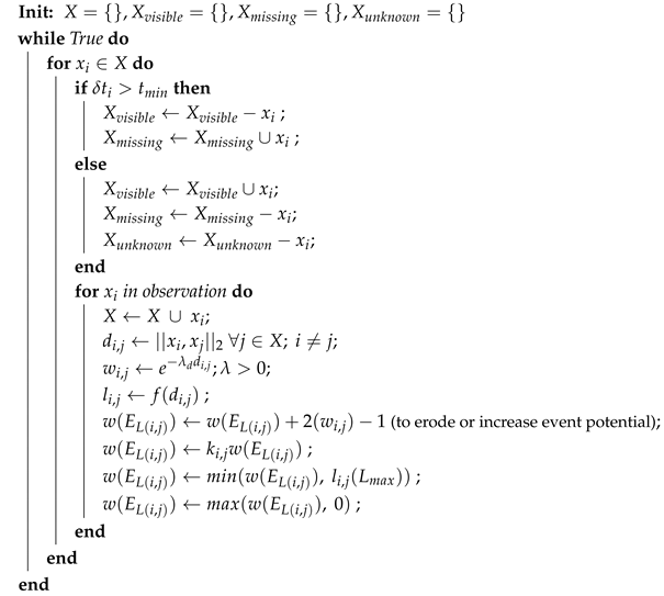 |
| where: | |
| Elapsed time since last observation for workpiece i | |
| User-defined time threshold to set the state of a workpiece as missing. This is set to two seconds in our experiments. | |
| Rate parameter for an exponential distribution to decide weight decay within a workpiece’s neighborhood (user-set parameter). Smaller values of have wider neighborhoods with softer weights, translating to a slower rate of increase in the linger counter within the neighborhood. Higher values have smaller neighborhoods with sharp weights within, translating to a sharp increase in the linger counter when workpieces are within the tight neighborhood. | |
| Weight attributed to the proximity factor modeled as an exponential decay for lower values at larger distances between workpieces. | |
| Weight representing domain knowledge on the likeliness of workpieces i and j getting stacked. Defaults to 1.0 if no bias is known. | |
| Edge in linger graph monitoring fit with every incoming observation. The longer is a workpiece observed within proximity, the higher the value. The edge weight is clipped as to keep the value bounded while being able to differentiate fit between workpieces within proximity. | |
| Weight for edge |
Appendix A.2. Event Graph
| Algorithm A2: Building event graph |
 |
| where: | |
| Edge in the event graph representing the likelihood of i and j getting stacked. | |
| Rate parameter to convert linger value to a probabilistic estimate through an exponential cumulative distribution function. Smaller values for translate to a slower rate of increase in the event likelihood whereas a higher value produces a higher rate of increase. Note that the rate at which the event likelihood reaches 1.0 can be controlled with both and . |
Appendix A.3. Dependency Graph
| Algorithm A3: Building dependency graph |
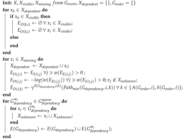 |
| where: | |
| Shortest path (based on edge weights) between nodes i and k in . | |
| Distance in terms of node separation between i and k in graph G. | |
| Separation penalty factor. | |
| Ancestors of node i in directed graph G. | |
| Siblings of node i in directed graph G. | |
| Edges in graph G. | |
| Local dependency graph built for mover’s field of view. |
References
- Zhong, R.Y.; Xu, X.; Klotz, E.; Newman, S.T. Intelligent manufacturing in the context of industry 4.0: A review. Engineering 2017, 3, 616–630. [Google Scholar] [CrossRef]
- Wang, S.; Wan, J.; Zhang, D.; Li, D.; Zhang, C. Towards smart factory for industry 4.0: A self-organized multi-agent system with big data based feedback and coordination. Comput. Netw. 2016, 101, 158–168. [Google Scholar] [CrossRef]
- Salkin, C.; Oner, M.; Ustundag, A.; Cevikcan, E. Conceptual framework for Industry 4.0. In Industry 4.0: Managing the Digital Transformation; Springer: Cham, Switzerland, 2018; pp. 3–23. [Google Scholar]
- Grau, D.; Caldas, C.H.; Haas, C.T.; Goodrum, P.M.; Gong, J. Assessing the impact of materials tracking technologies on construction craft productivity. Autom. Constr. 2009, 18, 903–911. [Google Scholar] [CrossRef]
- Brettel, M.; Friederichsen, N.; Keller, M.; Rosenberg, M. How virtualization, decentralization and network building change the manufacturing landscape: An Industry 4.0 Perspective. Int. J. Mech. Ind. Sci. Eng. 2014, 8, 37–44. [Google Scholar]
- Tao, F.; Cheng, J.; Qi, Q.; Zhang, M.; Zhang, H.; Sui, F. Digital twin-driven product design, manufacturing and service with big data. Int. J. Adv. Manuf. Technol. 2018, 94, 3563–3576. [Google Scholar] [CrossRef]
- Qi, Q.; Tao, F.; Zuo, Y.; Zhao, D. Digital twin service towards smart manufacturing. Procedia Cirp 2018, 72, 237–242. [Google Scholar] [CrossRef]
- Kasim, N.; Liwan, S.R.; Shamsuddin, A.; Zainal, R.; Kamaruddin, N.C. Improving on-site materials tracking for inventory management in construction projects. In Proceedings of the International Conference of Technology Management, Business and Entrepreneurship, Bandar Hilir, Melaka, Malaysia, 18–19 December 2012; pp. 2008–2013. [Google Scholar]
- Alaloul, W.S.; Liew, M.S.; Zawawi, N.A.W.A.; Mohammed, B.S. Industry revolution IR 4.0: Future opportunities and challenges in construction industry. MATEC web of conferences. EDP Sci. 2018, 203, 02010. [Google Scholar]
- Maskuriy, R.; Selamat, A.; Ali, K.N.; Maresova, P.; Krejcar, O. Industry 4.0 for the Construction Industry—How Ready Is the Industry? Appl. Sci. 2019, 9, 2819. [Google Scholar] [CrossRef]
- Niu, Y.; Lu, W.; Chen, K.; Huang, G.G.; Anumba, C. Smart construction objects. J. Comput. Civ. Eng. 2016, 30, 04015070. [Google Scholar] [CrossRef]
- Song, J.; Haas, C.T.; Caldas, C.H. Tracking the location of materials on construction job sites. J. Constr. Eng. Manag. 2006, 132, 911–918. [Google Scholar] [CrossRef]
- Navon, R.; Berkovich, O. An automated model for materials management and control. Constr. Manag. Econ. 2006, 24, 635–646. [Google Scholar] [CrossRef]
- Chandler, M.P. Improving the Construction Process Through Standardizing Daily Logs. Ph.D. Thesis, University of Florida, Gainesville, FL, USA, 2006. [Google Scholar]
- Rajaraman, M.; Philen, G.; Shimada, K. Tracking Tagged Inventory in Unstructured Environments through Probabilistic Dependency Graphs. Logistics 2019, 3, 21. [Google Scholar] [CrossRef]
- Spisakova, M.; Kozlovska, M. Application of RFID Technology on Construction Site–Case Study. In International Scientific Siberian Transport Forum; Springer: Cham, Switzerland, 2019; pp. 29–36. [Google Scholar]
- Oesterreich, T.D.; Teuteberg, F. Understanding the implications of digitisation and automation in the context of Industry 4.0: A triangulation approach and elements of a research agenda for the construction industry. Comput. Ind. 2016, 83, 121–139. [Google Scholar] [CrossRef]
- Kasim, N.; Shamsuddin, A.; Zainal, R.; Kamarudin, N.C. Implementation of RFID technology for real-time materials tracking process in construction projects. In Proceedings of the IEEE Colloquium on Humanities, Science and Engineering (CHUSER), Kota Kinabalu, Malaysia, 3–4 December 2012; pp. 699–703. [Google Scholar]
- Sardroud, J.M.; Limbachiya, M.; Saremi, A. Ubiquitous tracking and locating of construction resource using GIS and RFID. In Proceedings of the 6th GIS Conference and Exhibition (GIS 88), Tehran, Iran, 9–10 May 2010. [Google Scholar]
- Atkin, B.; Leiringer, R.; Wing, R. RFID Applications in Construction and Facilities Management. Electron. J. Inf. Technol. Constr. 2006, 11, 711–721. [Google Scholar]
- Lu, W.; Huang, G.Q.; Li, H. Scenarios for applying RFID technology in construction project management. Autom. Constr. 2011, 20, 101–106. [Google Scholar] [CrossRef]
- Kwon, W.; Park, J.H.; Lee, M.; Her, J.; Kim, S.H.; Seo, J.W. Robust Autonomous Navigation of Unmanned Aerial Vehicles (UAVs) for Warehouses’ Inventory Application. IEEE Robot. Autom. Lett. 2019, 5, 243–249. [Google Scholar] [CrossRef]
- Beul, M.; Droeschel, D.; Nieuwenhuisen, M.; Quenzel, J.; Houben, S.; Behnke, S. Fast autonomous flight in warehouses for inventory applications. IEEE Robot. Autom. Lett. 2018, 3, 3121–3128. [Google Scholar] [CrossRef]
- Teizer, J.; Vela, P.A. Personnel tracking on construction sites using video cameras. Adv. Eng. Inf. 2009, 23, 452–462. [Google Scholar] [CrossRef]
- Teizer, J. Status quo and open challenges in vision-based sensing and tracking of temporary resources on infrastructure construction sites. Adv. Eng. Inf. 2015, 29, 225–238. [Google Scholar] [CrossRef]
- Fang, Q.; Li, H.; Luo, X.; Ding, L.; Rose, T.M.; An, W.; Yu, Y. A deep learning-based method for detecting non-certified work on construction sites. Adv. Eng. Inf. 2018, 35, 56–68. [Google Scholar] [CrossRef]
- Kereri, J.O.; Turner, B.S. Use of technology in material tracking in the construction industry business. Afr. J. Bus. Manag. 2018, 4, 53–60. [Google Scholar]
- Isard, M.; Blake, A. A smoothing filter for condensation. In European Conference on Computer Vision; Springer: Berlin/Heidelberg, Germany, 1998; pp. 767–781. [Google Scholar]
- Fox, D.; Burgard, W.; Thrun, S. Markov localization for mobile robots in dynamic environments. J. Artif. Intell. Res. 1999, 11, 391–427. [Google Scholar] [CrossRef]
- Gadeyne, K.; Bruyninckx, H. Markov techniques for object localization with force-controlled robots. In Proceedings of the 10th International Conference on Advanced Robotics, Budapest, Hungary, 22–25 August 2001. [Google Scholar]
- Chong, C.Y.; Mori, S.; Reid, D.B. Forty years of multiple hypothesis tracking-a review of key developments. In Proceedings of the 21st International Conference on Information Fusion (FUSION), Cambridge, UK, 10–13 July 2018; pp. 452–459. [Google Scholar]
- Kim, C.; Li, F.; Ciptadi, A.; Rehg, J.M. Multiple hypothesis tracking revisited. In Proceedings of the IEEE International Conference on Computer Vision, Santiago, Chile, 11–18 December 2015; pp. 4696–4704. [Google Scholar]
- Mueller, E.T. Common-Sense Reasoning: An Event Calculus Based Approach; Morgan Kaufmann: Burlington, MA, USA, 2014. [Google Scholar]
- Fire, A.; Zhu, S.C. Inferring Hidden Statuses and Actions in Video by Causal Reasoning. In Proceedings of the IEEE Conference on Computer Vision and Pattern Recognition Workshops, Honolulu, HI, USA, 21–26 July 2017; pp. 48–56. [Google Scholar]
- Xu, Y.; Qin, L.; Liu, X.; Xie, J.; Zhu, S.C. A causal and-or graph model for visibility fluent reasoning in tracking interacting objects. In Proceedings of the IEEE Conference on Computer Vision and Pattern Recognition, Salt Lake City, UT, USA, 18–22 June 2018; pp. 2178–2187. [Google Scholar]
- Fire, A.; Zhu, S.C. Learning perceptual causality from video. ACM Trans. Intell. Syst. Technol. TIST 2015, 7, 1–22. [Google Scholar] [CrossRef]
- Quigley, M.; Conley, K.; Gerkey, B.; Faust, J.; Foote, T.; Leibs, J.; Wheeler, R.; Ng, A.Y. ROS: An open-source Robot Operating System. In Proceedings of the ICRA Workshop on Open Source Software, Kobe, Japan, 12–17 May 2009; Volume 3, p. 5. [Google Scholar]
- Gunnarsson, K.T.; Prinz, F.B. CAD model-based localization of parts in manufacturing. Computer 1987, 8, 66–74. [Google Scholar] [CrossRef]
- Yau, H.T.; Menq, C.H. An automated dimensional inspection environment for manufactured parts using coordinate measuring machines. Int. J. Prod. Res. 1992, 30, 1517–1536. [Google Scholar] [CrossRef]
- Rajaraman, M.; Dawson-Haggerty, M.; Shimada, K.; Bourne, D.A. Automated workpiece localization for robotic welding. In Proceedings of the IEEE International Conference on Automation Science and Engineering (CASE), Madison, WI, USA, 17–20 August 2013; pp. 681–686. [Google Scholar]
- Thrun, S.; Fox, D.; Burgard, W.; Dellaert, F. Robust Monte Carlo localization for mobile robots. Artif. Intell. 2001, 128, 99–141. [Google Scholar] [CrossRef]
- Petrovskaya, A.; Khatib, O.; Thrun, S.; Ng, A.Y. Bayesian estimation for autonomous object manipulation based on tactile sensors. In Proceedings of the IEEE International Conference on Robotics and Automation (ICRA), Orlando, FL, USA, 15–19 May 2006; pp. 707–714. [Google Scholar]
- Scheidegger, A.P.G.; Pereira, T.F.; de Oliveira, M.L.M.; Banerjee, A.; Montevechi, J.A.B. An introductory guide for hybrid simulation modelers on the primary simulation methods in industrial engineering identified through a systematic review of the literature. Comput. Ind. Eng. 2018, 124, 474–492. [Google Scholar] [CrossRef]
- Agnusdei, G.; Gnoni, M.; Tornese, F. Modelling and Simulation Tools for Integrating Forward and Reverse Logistics: A Literature Review. In Proceedings of the 31st European Modeling and Simulation Symposium (EMSS), Lisbon, Portugal, 18–20 September 2019; pp. 317–326. [Google Scholar]
© 2020 by the authors. Licensee MDPI, Basel, Switzerland. This article is an open access article distributed under the terms and conditions of the Creative Commons Attribution (CC BY) license (http://creativecommons.org/licenses/by/4.0/).

