Travel Time Prediction in a Multimodal Freight Transport Relation Using Machine Learning Algorithms


Abstract
:1. Introduction
2. Literature Review
3. Methodology
3.1. Choice of Learning Algorithms
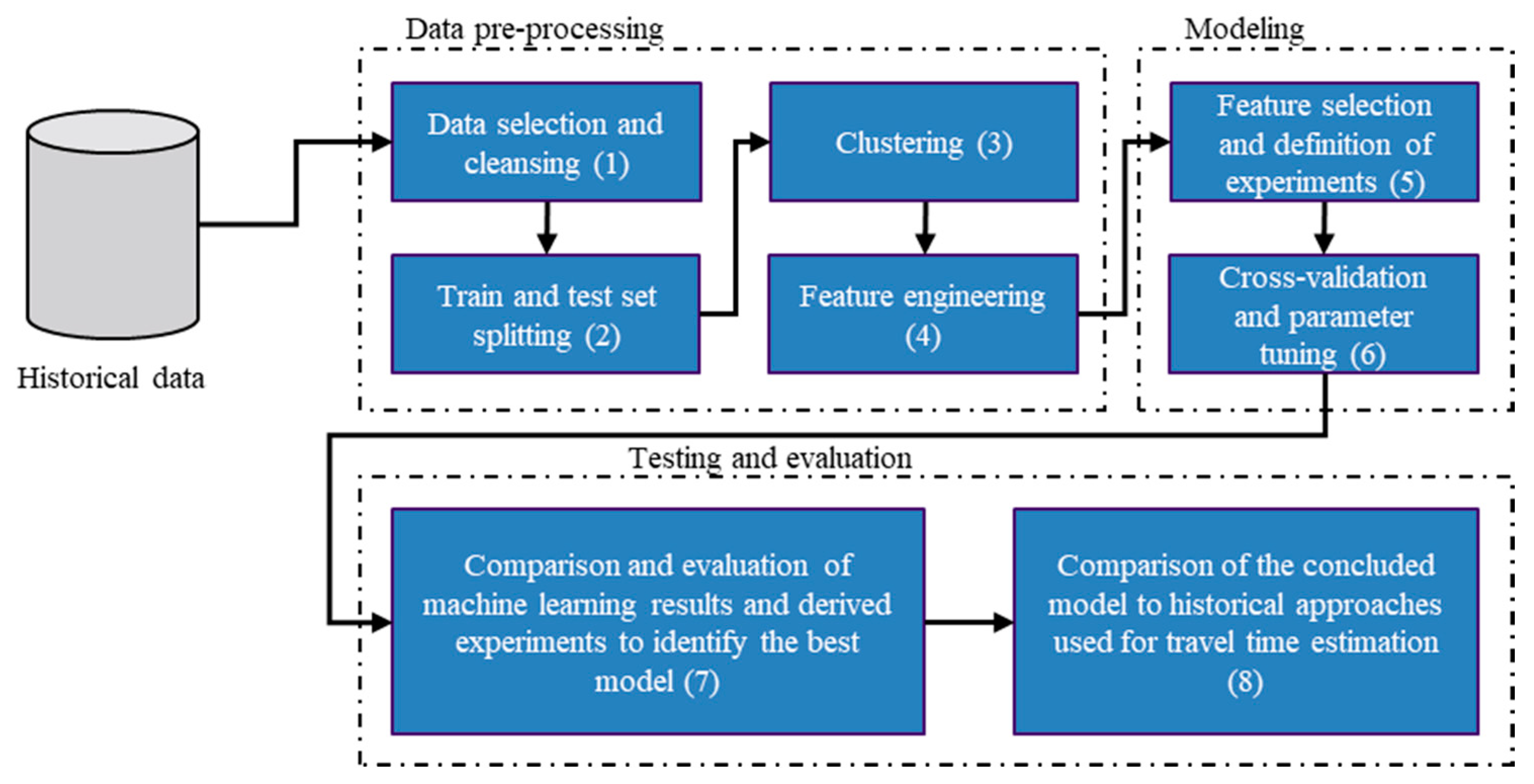
3.2. Framework
4. Use-Case and Data Generation
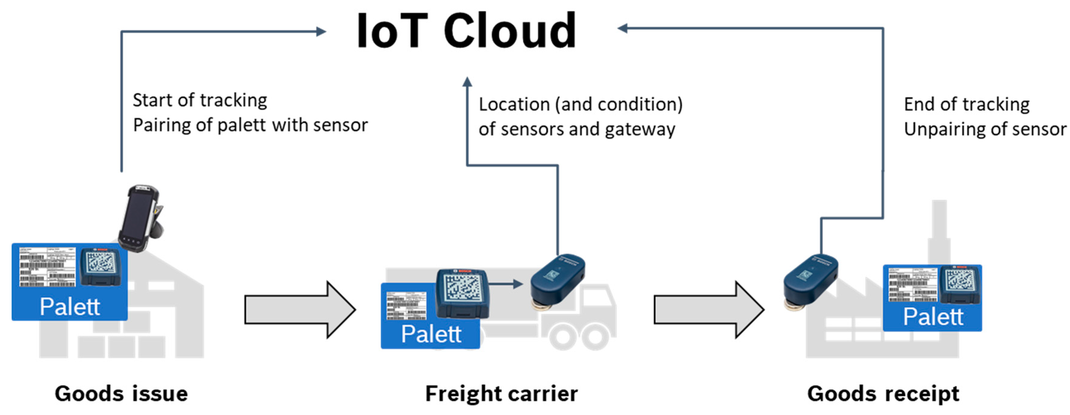
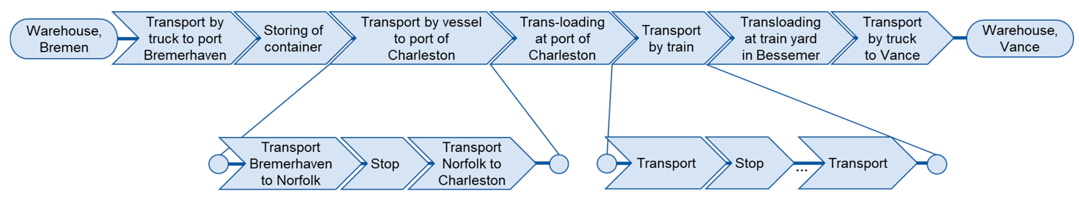
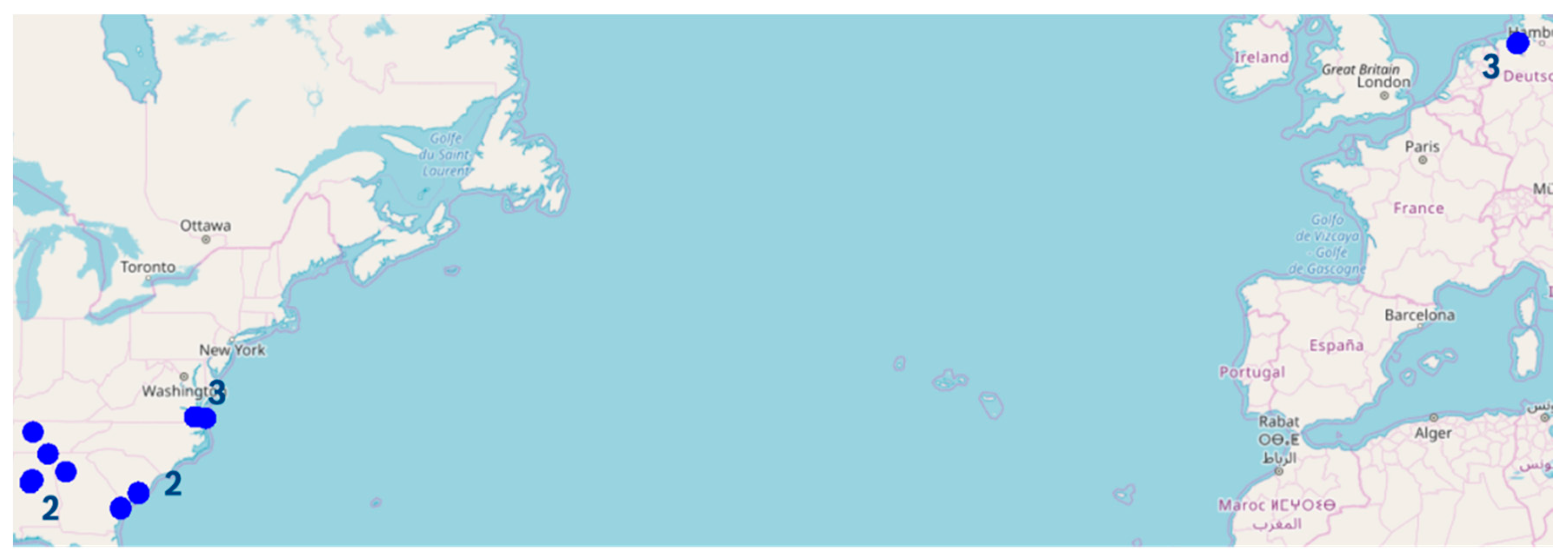
4.1. Use-Case Description
4.2. Data Generation and Description
5. Data Pre-Processing
5.1. Data Cleansing
- If the test pairings have no GPS transmissions falling within its destination geo-fence, they will be removed. This means that the goods have never reached the destination.
- If transmissions have a latitude and longitude set to 0°, the transmission will be removed and ignored as it implies the absence of a GPS signal.
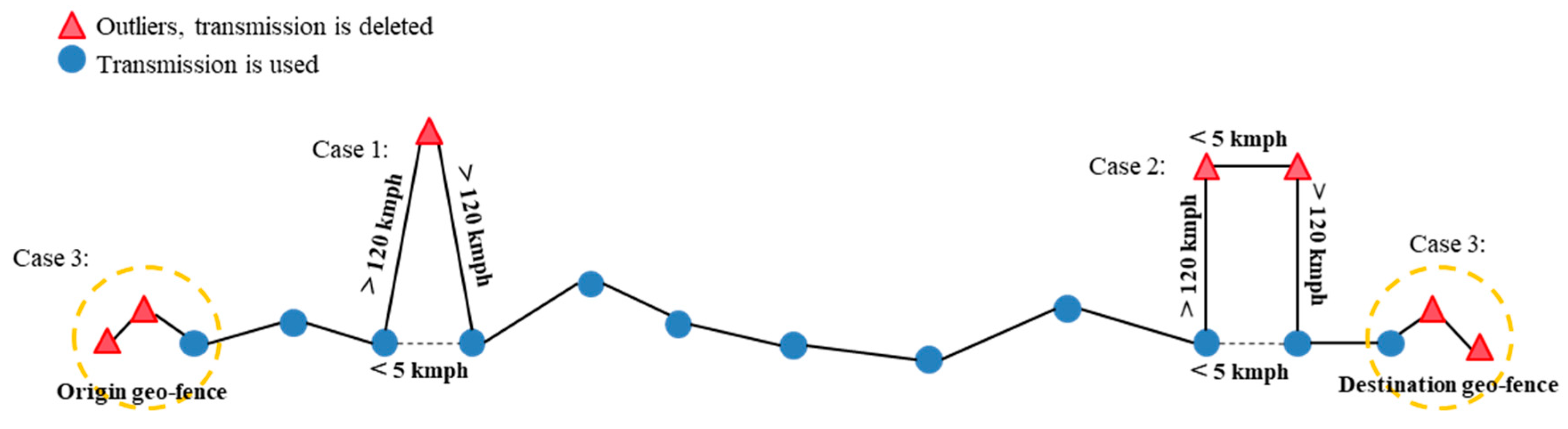
- While storing the containers at the ports and at other intermediate stops, outliers have been detected. To identify outliers, the speed between two consecutive stops has been used, which exceeded 120 kmph in this case. Case 1 in Figure 4 shows one outlier where the speed exceeds more than 120 kmph to the previous and following transmission. At the same time, the speed between the transmissions before and after the outlier is significantly smaller, with a speed below 5 kmph. In Case 2 of Figure 4, two consecutive outliers have been detected, which are relatively close to each other. The speed between the outliers is below 5 kmph, while the speed to the previous and following transmission again exceeds 120 kmph. As before, the speed before and after the outliers is below 5 kmph. The transmissions identified as outliers based on the described rules have been removed, as shown in Figure 4.
- As only the transport itself should be considered, data points other than the last transmission in the origin geo-fence and the first transmission in the destination geo-fence are removed. This situation is shown in Figure 4, Case 3.
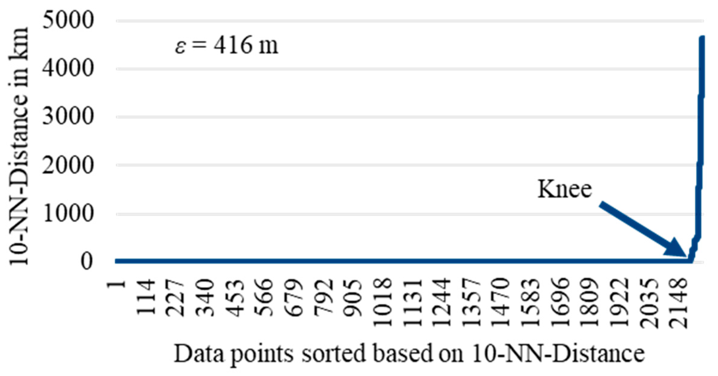
5.2. Clustering for Route Identification
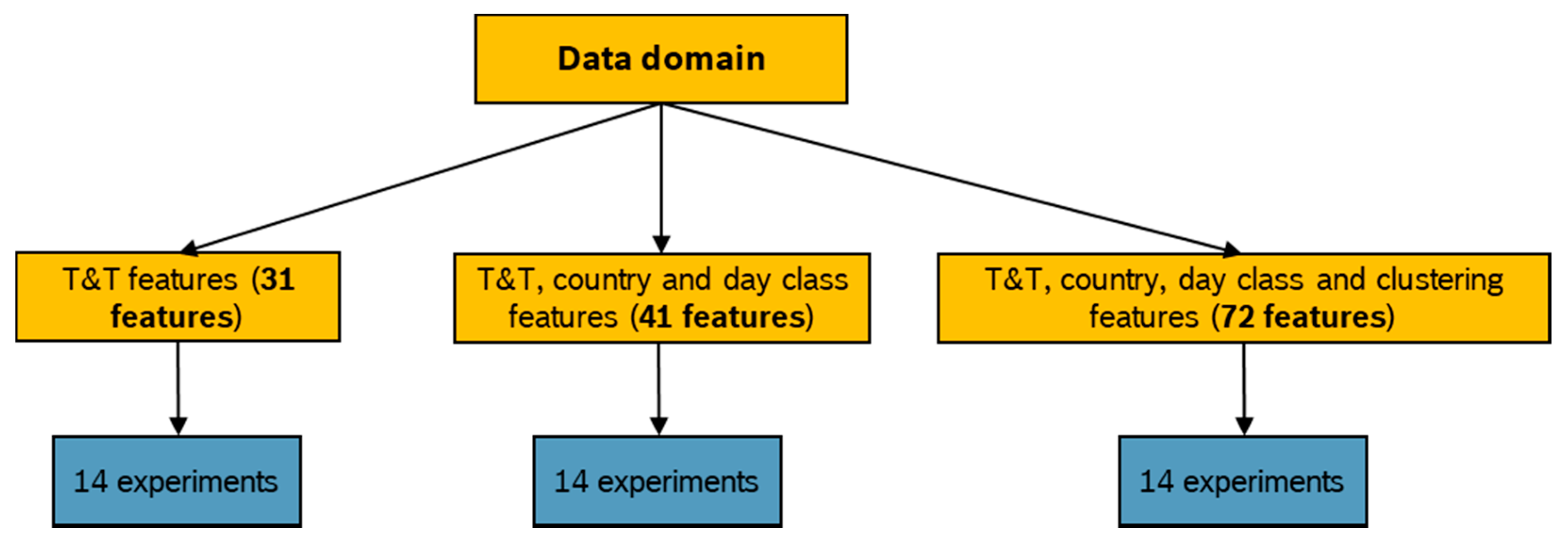
5.3. Feature Engineering and Data Transformation
6. Modelling
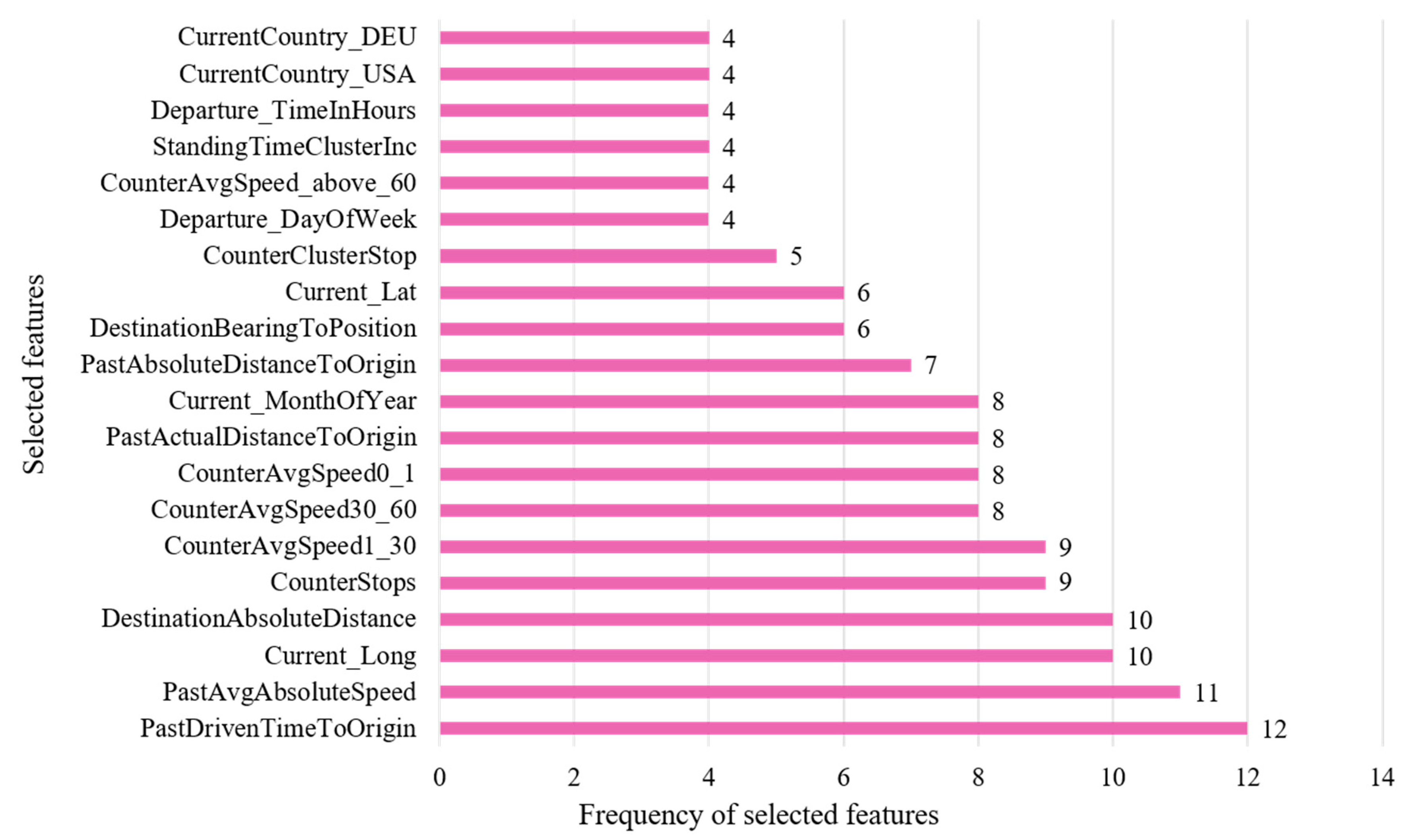
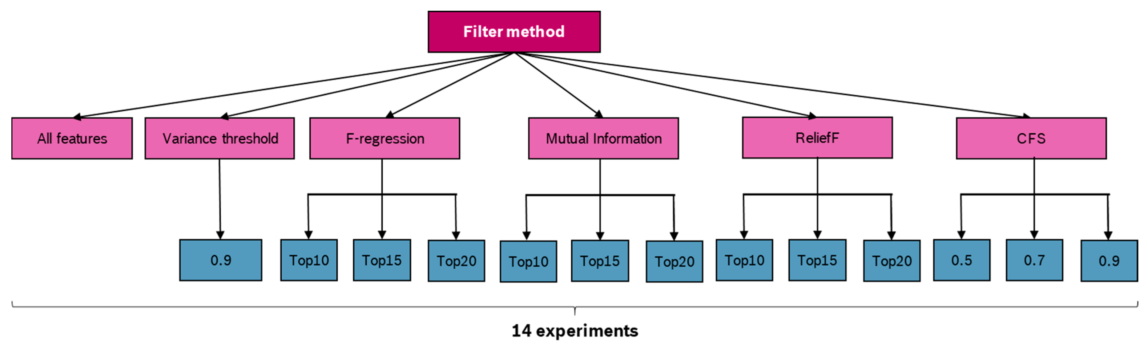
6.1. Feature Selection
- An easily interpretable method is one that uses a variance threshold. Features with a variation below a certain cut-off value have been removed. Therefore, for each feature, we identify the value with the highest frequency and divide it by the number of data points to calculate the percentage. In our study, features with at least 90% of their instances remaining constant are removed, and the threshold is set to 0.9 [49] (p. 509).
- F-regression runs an F test for each feature (regressor), relevant for travel time prediction apart from the target. Therefore, the variance of each feature and the target is calculated. The ratio provides the F value, which is then transformed into a p-value using the F probability distribution. Consequently, the p-value scores the individual effect of each regressor [50] (p. 629).
- The mutual information method considers non-linear dependencies as well as linear relationships by calculating the distance between the probability distributions of two features [51] (pp. 175–178). A feature selection procedure has been conducted by ranking the calculated mutual information of each feature.
- As per [48], the feature selection based on the ReliefF algorithm provided a superior performance in previous research. The applied algorithm considers feature interaction and is implemented in a way so that both continuous and categorical features can be processed. The algorithm calculates weights for each features, which are used for ranking them. Therefore, for a number of iterations, a random instance of all feature, which represents a row in the data, is chosen. For this chosen instance, the instances with the nearest hit and miss are identified based on the Manhattan distance. Finally, a diff-function is used to calculate the weight for each feature by subtracting it from the weight of the previous iteration. In the first iteration, the weight is set to zero. A higher weight means a better feature based on the ReliefF algorithm [48] (p. 487).
- Correlation based feature selection (CFS) is another well-known filter method, which calculates the correlation between predictor and target and then filters out features with a correlation below a given threshold [52] (pp. 361–362).
6.2. Validation and Parameter Tuning
7. Evaluation
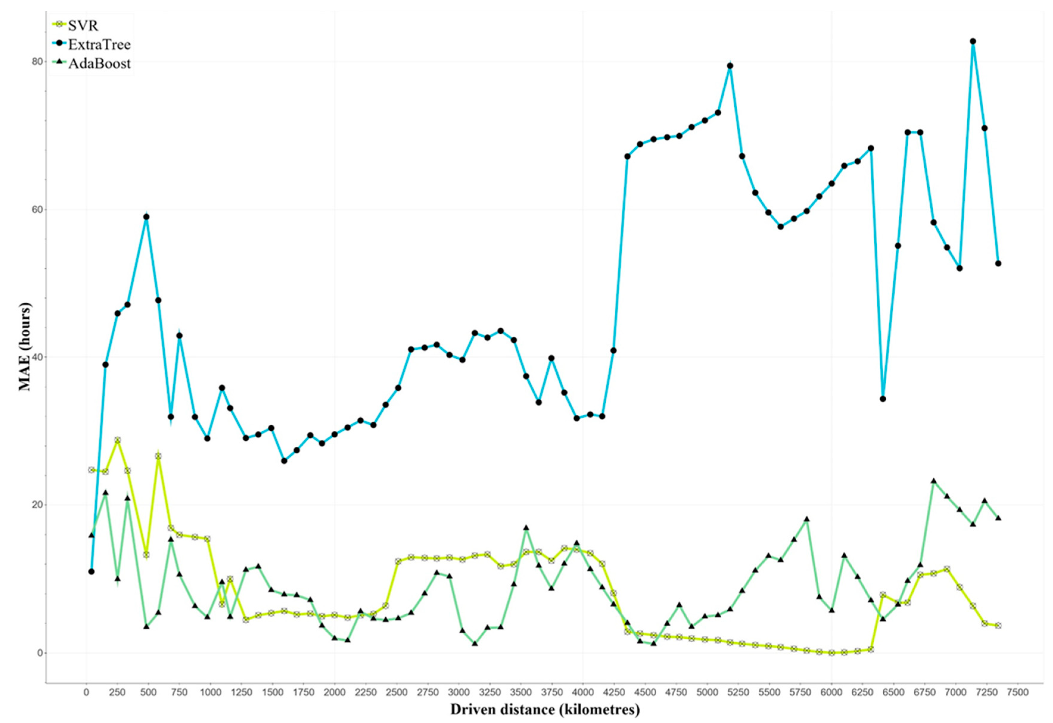
7.1. Evaluation of Machine Learning Models
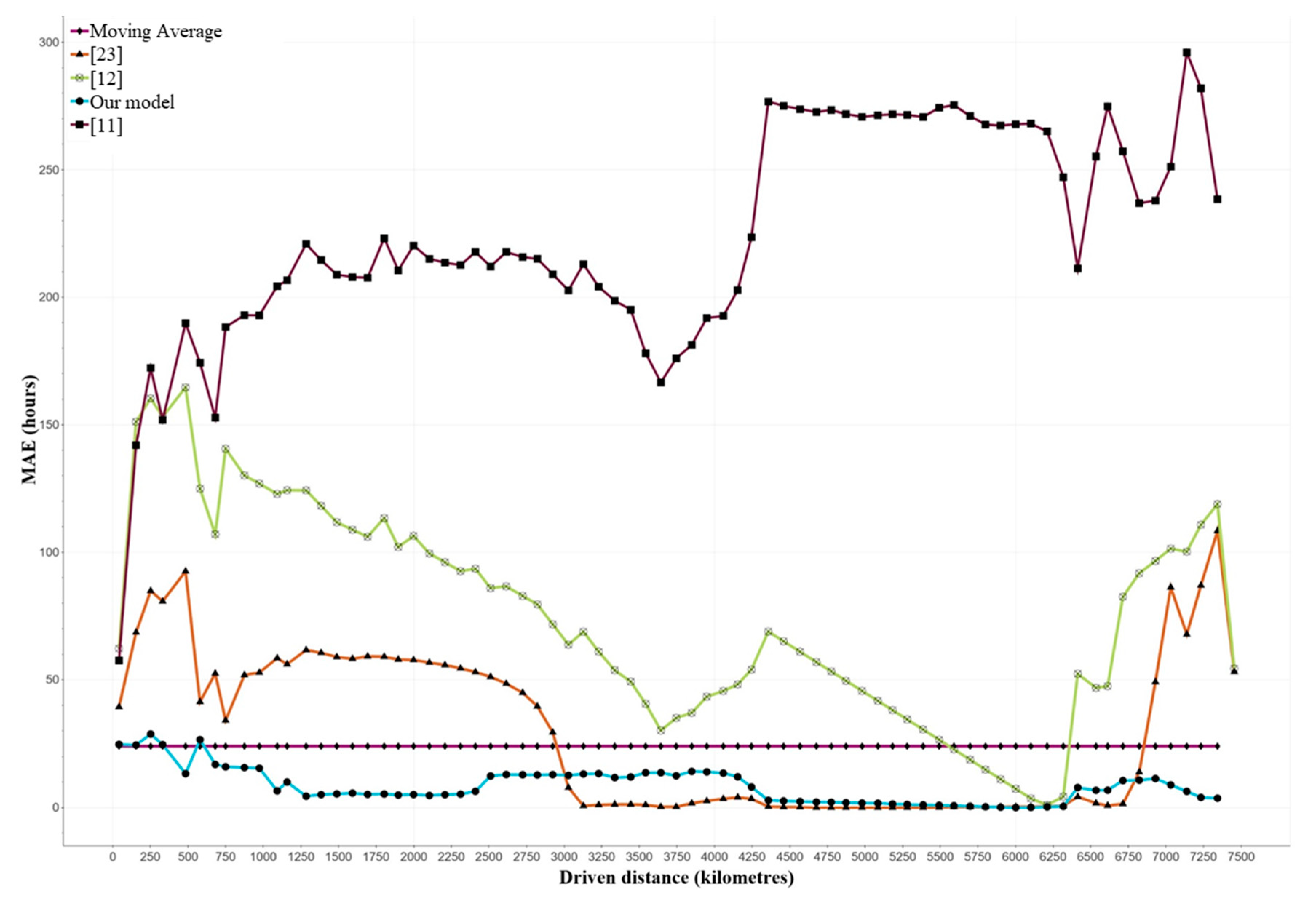
7.2. Comparison to Average-Based Approaches
- We are assuming that t transports have been completed. determines one specific transport with . is then the currently observed transport for prediction.
- We also assume as the number of transmissions per transport . Then determines the number of transmissions of the current transport with .
- : Actual Travel Time of transport j.
- : Actual Travel Time of transport j from transmission i to the destination.
- : Estimated Travel Time of transport j and from transmission i.
- : Actual Time of Departure of transport j.
- : Estimated Time of Arrival of transport j and from transmission i.
8. Conclusions
Author Contributions
Funding
Conflicts of Interest
References
- Parolas, I.; Tavasszy, L.; Kourounioti, I.; van Duin, R. Predicition of Vessels’ estimated time of arrival (ETA) using machine learning: A port of rotterdam case study. In Proceedings of the 96th Annual Meeting of the Transportation Research, Washington, DC, USA, 8–12 January 2017; pp. 8–12. [Google Scholar]
- Masiero, L.P.; Casanova, M.A.; de Carvalho, M.T.M. Travel time prediction using machine learning. In Proceedings of the 4th ACM SIGSPATIAL International Workshop on Computational Transportation Science, Chicago, IL, USA, 1 November 2011; Thakuriah, P., Ed.; ACM: New York, NY, USA, 2011; pp. 34–38. [Google Scholar]
- Teucke, M.; Broda, E.; Börold, A.; Freitag, M. Using Sensor-Based Quality Data in Automotive Supply Chains. Machines 2018, 6, 53. [Google Scholar] [CrossRef] [Green Version]
- Lin, H.-E.; Taylor, M.A.P.; Zito, R. A review of travel-time prediction in transport and logistics. In Proceedings of the 6th Eastern Asia Society for Transportation Studies (EASTS) Conference, Bangkok, Thailand, 21–24 September 2005; pp. 1433–1448. [Google Scholar]
- Zijm, H.; Klumpp, M.; Regattieri, A.; Heragu, S. Operations, Logistics and Supply Chain Management: Definitions and Objectives. In Operations, Logistics and Supply Chain Management; Zijm, H., Klumpp, M., Regattieri, A., Heragu, S., Eds.; Springer: Cham, Germany, 2019; pp. 27–42. [Google Scholar]
- Sommerfeld, D.; Teucke, M.; Freitag, M. Identification of Sensor Requirements for a Quality Data-based Risk Management in Multimodal Supply Chains. Procedia CIRP 2018, 72, 563–568. [Google Scholar] [CrossRef]
- Farahani, P.; Meier, C.; Wilke, J. Digital Supply Chain Management. 2020 Vision: Whitepaper. Available online: https://www.sap.com/documents/2017/04/88e5d12e-b57c-0010-82c7-eda71af511fa.html (accessed on 17 November 2019).
- Li, X.; Bai, R. Freight Vehicle Travel Time Prediction Using Gradient Boosting Regression Tree. In Proceedings of the 15th IEEE International Conference on Machine Learning and Applications (ICMLA), Anaheim, CA, USA, 18–20 December 2016; IEEE: Piscataway, NJ, USA, 2016; pp. 1010–1015. [Google Scholar]
- Vlahogianni, E.I.; Karlaftis, M.G.; Golias, J.C. Short-term traffic forecasting: Where we are and where we’re going. Transp. Res. Part C Emerg. Technol. 2014, 43, 3–19. [Google Scholar] [CrossRef]
- Altinkaya, M.; Zontul, M. Urban bus arrival time prediction: A review of computational models. Int. J. Rec. Technol. Eng. 2013, 2, 164–169. [Google Scholar]
- Singla, L.; Bhatia, P. GPS based bus tracking system. In Proceedings of the 2015 International Conference on Computer, Communication and Control (IC4), Indore, India, 10–12 September 2015; IEEE: Piscataway, NJ, USA, 2015; pp. 1–6. [Google Scholar]
- Čelan, M.; Lep, M. Bus-arrival time prediction using bus network data model and time periods. Future Gener. Comput. Syst. 2018. [Google Scholar] [CrossRef]
- Kwon, J.; Petty, K. Travel time prediction algorithm scalable to freeway networks with many nodes with arbitrary travel routes. Transp. Res. Rec. 2005, 1935, 147–153. [Google Scholar] [CrossRef]
- Shalaby, A.; Farhan, A. Prediction Model of Bus Arrival and Departure Times Using AVL and APC Data. J. Public Transp. 2004, 7, 41–61. [Google Scholar] [CrossRef] [Green Version]
- Chen, M.; Liu, X.; Xia, J.; Chien, S.I. A Dynamic Bus-Arrival Time Prediction Model Based on APC Data. Comput.-Aided Civ. Infrastruct. Eng. 2004, 19, 364–376. [Google Scholar] [CrossRef]
- Vanajakshi, L.; Subramanian, S.C.; Sivanandan, R. Travel Time Prediction under Heterogeneous Traffic Conditions Using Global Positioning System Data from Buses. IET Intell. Transp. Syst. 2009, 3, 1–9. [Google Scholar] [CrossRef]
- Chien, S.I.-J.; Kuchipudi, C.M. Dynamic Travel Time Prediction with Real-Time and Historic Data. J. Transp. Eng. 2003, 129, 608–616. [Google Scholar] [CrossRef]
- Fan, W.; Gurmu, Z. Dynamic Travel Time Prediction Models for Buses Using Only GPS Data. Int. J. Transp. Sci. Technol. 2015, 4, 353–366. [Google Scholar] [CrossRef]
- Yu, B.; Lam, W.H.K.; Tam, M.L. Bus arrival time prediction at bus stop with multiple routes. Transp. Res. Part C Emerg. Technol. 2011, 19, 1157–1170. [Google Scholar] [CrossRef]
- Zychowski, A.; Junosza-Szaniawski, K.; Kosicki, A. Travel Time Prediction for Trams in Warsaw. In Proceedings of the 10th International Conference on Computer Recognition Systems (CORES), Polanica Zdroj, Poland, 22–24 May 2017; Kurzynski, M., Wozniak, M., Burduk, R., Eds.; Springer International Publishing: Cham, Germany, 2018; pp. 53–61. [Google Scholar]
- Sun, X.; Zhang, H.; Tian, F.; Yang, L. The Use of a Machine Learning Method to Predict the Real-Time Link Travel Time of Open-Pit Trucks. Math. Probl. Eng. 2018, 2018, 4368045. [Google Scholar] [CrossRef] [Green Version]
- Servos, N.; Teucke, M.; Freitag, M. Travel Time Prediction for Multimodal Freight Transports using Machine Learning. In Proceedings of the 23th International Conference on Material Handling, Constructions and Logistics (MHCL), Vienna, Austria, 18–20 September 2019; Kartnig, G., Zrnić, N., Bošnjak, S., Eds.; University of Belgrade Faculty of Mechanical Engineering: Belgrade, Serbia, 2019; pp. 223–228. [Google Scholar]
- Heywood, C.; Connor, C.; Browning, D.; Smith, M.C.; Wang, J. GPS tracking of intermodal transportation: System integration with delivery order system. In Proceedings of the 2009 IEEE Systems and Information Engineering Design Symposium, Charlottesville, VA, USA, 24 April 2009; Louis, G.E., Crowther, K.G., Eds.; IEEE: Charlottesville, VA, USA, 2009; pp. 191–196. [Google Scholar]
- Kisgyörgy, L.; Rilett, L.R. Travel Time prediction by Advanced Neural Network. Periodica Polytech. Ser. Civ. Eng. 2002, 46, 15–32. [Google Scholar]
- Wu, C.-H.; Ho, J.-M.; Lee, D.T. Travel-Time Prediction with Support Vector Regression. IEEE Trans. Intell. Transp. Syst. 2004, 5, 276–281. [Google Scholar] [CrossRef] [Green Version]
- Šemanjski, I. Potenial of Big Data in Forecasting Travel Times. Promet-Traffic Transp. 2015, 27, 515–528. [Google Scholar] [CrossRef] [Green Version]
- Zhang, Y.; Haghani, A. A gradient boosting method to improve travel time prediction. Transp. Res. Part C Emerg. Technol. 2015, 58, 308–324. [Google Scholar] [CrossRef]
- Siripanpornchana, C.; Panichpapiboon, S.; Chaovalit, P. Travel-time prediction with deep learning. In Proceedings of the 2016 IEEE Region 10 Conference (TENCON), Marina Bay Sands, Singapore, 22–25 November 2016; IEEE: Piscataway, NJ, USA, 2016; pp. 1859–1862. [Google Scholar]
- Jeong, R.; Laurence, R.R. Bus arrival time prediction using artificial neural network model. In Proceedings of the 7th International IEEE Conference on Intelligent Transportation Systems, Washington, WA, USA, 3–7 October 2004; IEEE: Piscataway, NJ, USA, 2004; pp. 988–993. [Google Scholar]
- Pan, J.; Dai, X.; Xu, X.; Li, Y. A Self-learning algorithm for predicting bus arrival time based on historical data model. In Proceedings of the 2012 IEEE 2nd International Conference on Cloud Computing and Intelligence Systems, Hangzhou, China, 30 October–1 November 2012; Li, D., Yang, F., Ren, F., Wang, W., Eds.; IEEE: Piscataway, NJ, USA, 2012; pp. 1112–1116. [Google Scholar]
- Dong, J.; Zou, L.; Zhang, Y. Mixed model for prediction of bus arrival times. In Proceedings of the 2013 IEEE Congress on Evolutionary Computation (CEC), Cancún, Mexico, 20–23 June 2013; IEEE: Piscataway, NJ, USA, 2013; pp. 2918–2923. [Google Scholar]
- Treethidtaphat, W.; Pattara-Atikom, W.; Khaimook, S. Bus Arrival Time Prediction at Any Distance of Bus Route Using Deep Neural Network Model. In Proceedings of the 20th International Conference on Intelligent Transportation Systems, Mielparque Yokohama in Yokohama, Kanagawa, Japan, 16–19 October 2017; IEEE: Piscataway, NJ, USA, 2017; pp. 988–992. [Google Scholar]
- Zhang, J.; Gu, J.; Guan, L.; Zhang, S. Method of predicting bus arrival time based on MapReduce combining clustering with neural network. In Proceedings of the IEEE 2nd International Conference on Big Data Analysis (ICBDA), Beijing, China, 10–12 March 2017; IEEE: Piscataway, NJ, USA, 2017; pp. 296–302. [Google Scholar]
- Yang, M.; Chen, C.; Wang, L.; Yan, X.; Zhou, L. Bus Arrival Time Prediction using Support Vector Machine with Genetic Algorithm. Neural Netw. World 2016, 26, 205–217. [Google Scholar] [CrossRef] [Green Version]
- Patnaik, J.; Chien, S.; Bladikas, A. Estimation of Bus Arrival Times Using APC Data. J. Public Transp. 2004, 7, 1–20. [Google Scholar] [CrossRef] [Green Version]
- Kern, C.S.; de Medeiros, I.P.; Yoneyama, T. Data-driven aircraft estimated time of arrival prediction. In Proceedings of the 9th Annual IEEE International Systems Conference (SysCon), Vancouver, BC, Canada, 13–16 April 2015; IEEE: Piscataway, NJ, USA, 2015; pp. 727–733. [Google Scholar]
- Kee, C.Y.; Wong, L.-P.; Khader, A.T.; Hassan, F.H. Multi-label classification of estimated time of arrival with ensemble neural networks in bus transportation network. In Proceedings of the 2nd IEEE International Conference on Intelligent Transportation Engineering (ICITE), Singapore, 1–3 September 2017; IEEE: Piscataway, NJ, USA, 2017; pp. 150–154. [Google Scholar]
- Cortes, C.; Vapnik, V. Support-Vector Networks. Mach. Learn. 1995, 20, 273–297. [Google Scholar] [CrossRef]
- Barbour, W.; Martinez Mori, J.C.; Kuppa, S.; Work, D.B. Prediction of arrival times of freight traffic on US railroads using support vector regression. Transp. Res. Part C Emerg. Technol. 2018, 93, 211–227. [Google Scholar] [CrossRef] [Green Version]
- Awad, M.; Khanna, R. Support Vector Regression. In Efficient Learning Machines: Theories, Concepts, and Applications for Engineers and System Designers; Awad, M., Khanna, R., Eds.; Apress: Berkeley, CA, USA, 2015; pp. 67–80. [Google Scholar]
- Geurts, P.; Ernst, D.; Wehenkel, L. Extremely randomized trees. Mach. Learn. 2006, 63, 3–42. [Google Scholar] [CrossRef] [Green Version]
- Kadiyala, A.; Kumar, A. Applications of python to evaluate the performance of decision tree-based boosting algorithms. Environ. Prog. Sustain. Energy 2018, 37, 618–623. [Google Scholar] [CrossRef]
- Schapire, R.E. Explaining AdaBoost. In Empirical Inference; Schölkopf, B., Luo, Z., Vovk, V., Eds.; Springer: Berlin/Heidelberg, Germany, 2013; pp. 37–52. [Google Scholar]
- Van der Spoel, S.; Amrit, C.; van Hillegersberg, J. Predictive analytics for truck arrival time estimation: A field study at a European distribution centre. Int. J. Prod. Res. 2017, 55, 5062–5078. [Google Scholar] [CrossRef]
- Swamynathan, M. Mastering Machine Learning with Python in Six Steps. A Practical Implementation Guide to Predictive Data Analytics Using Python; Apress: New York, NY, USA, 2017. [Google Scholar]
- Yang, J.; Xu, J.; Xu, M.; Zheng, N.; Chen, Y. Predicting Next Location Using a Variable Order Markov model. In Proceedings of the 5th ACM SIGSPATIAL International Workshop on GeoStreaming (IWGS), Dallas, TX, USA, 4 November 2014; Zhang, C., Basalamah, A., Hendawi, A., Eds.; ACM: New York, NY, USA, 2014; pp. 37–42. [Google Scholar]
- Ester, M.; Kriegel, H.-P.; Sander, J.; Xu, X. A density-based algorithm for discovering clusters in large spatial databases with noise. In Proceedings of the 2nd International Conference on Knowledge Discovery and Data Mining (KDD), Portland, OR, USA, 2–4 August 1996; Simoudis, E., Han, J., Fayyad, U., Eds.; AAAI Press: Palo Alto, CA, USA, 1996; pp. 226–231. [Google Scholar]
- Bolón-Canedo, V.; Sánchez-Maroño, N.; Alonso-Betanzos, A. A review of feature selection methods on synthetic data. Knowl. Inf. Syst. 2013, 34, 483–519. [Google Scholar] [CrossRef]
- He, X.; Cai, D.; Niyogi, P. Laplacian score for feature selection. In Proceedings of the 19th Advances in Neural Information Processing Systems (NIPS) Conference, Vancouver, BC, Canada, 5–10 December 2006; Weiss, Y., Schölkopf, B., Eds.; MIT Press: Cambridge, UK, 2006; pp. 507–514. [Google Scholar]
- Omer Fadl Elssied, N.; Ibrahim, O.; Hamza Osman, A. A Novel Feature Selection Based on One-Way ANOVA F-Test for E-Mail Spam Classification. Res. J. Appl. Sci. Eng. Technol. 2014, 7, 625–638. [Google Scholar] [CrossRef]
- Vergara, J.R.; Estévez, P.A. A review of feature selection methods based on mutual information. Neural Comput. Appl. 2014, 24, 175–186. [Google Scholar] [CrossRef]
- Hall, M.A. Correlation-based Feature Selection for Discrete and Numeric Class Machine Learning. In Proceedings of the 7th International Conference on Machine Learning (ICML), San Francisco, CA, USA, 29 June–2 July 2000; pp. 359–366. [Google Scholar]
- Mukaka, M.M. A guide to appropriate use of Correlation coefficient in medical research. Malawi Med. J. 2012, 24, 69–71. [Google Scholar]


| Column | Description |
|---|---|
| Unit load ID | Unique identifier of paired transport unit load |
| Start/End of tracking | Pairing and un-pairing Unix time in seconds |
| Gateway ID | Unique identifier of transmitting gateway |
| Last Update | Unix time of transmission in milliseconds |
| Latitude, longitude | Geo-location of the last update |
| Temperature, humidity | Quality related data of sensor of last update |
| Data Source | Description |
|---|---|
| Tracking system (T&T) | Features derived from tracking data without complex transformations and further data sources |
| Country (Coun) | Country derived from a geo-coding application programming interface (API) based on geo coordinates |
| Day Class (DC) | Features considering the day class derived from the country and information considering public holidays |
| Clustering (Cl) | Features derived from the clustering |
| Feature | Description | Cat. | Data |
|---|---|---|---|
| AbsoluteDistanceToPrevious | Absolute distance in kilometers from the previous position to the position. | No | T&T |
| AvgSpeedPrevious | Average speed from current transmission to previous transmission as quotient of AbsoluteDistanceToPrevious and DrivenTimePrevious. | No | T&T |
| CounterAvgSpeed0_1, CounterAvgSpeed1_30, CounterAvgSpeed30_60 and CounterAvgSpeed_above_60 | Counter of the number of AvgSpeedPrevious from departure to the current transmission from 0 to 1 kmph, 1 to 30 kmph, 30 to 60 kmph, and over 60 kmph derived from the data. Those features are based on business knowledge to represent traffic conditions. | No | T&T |
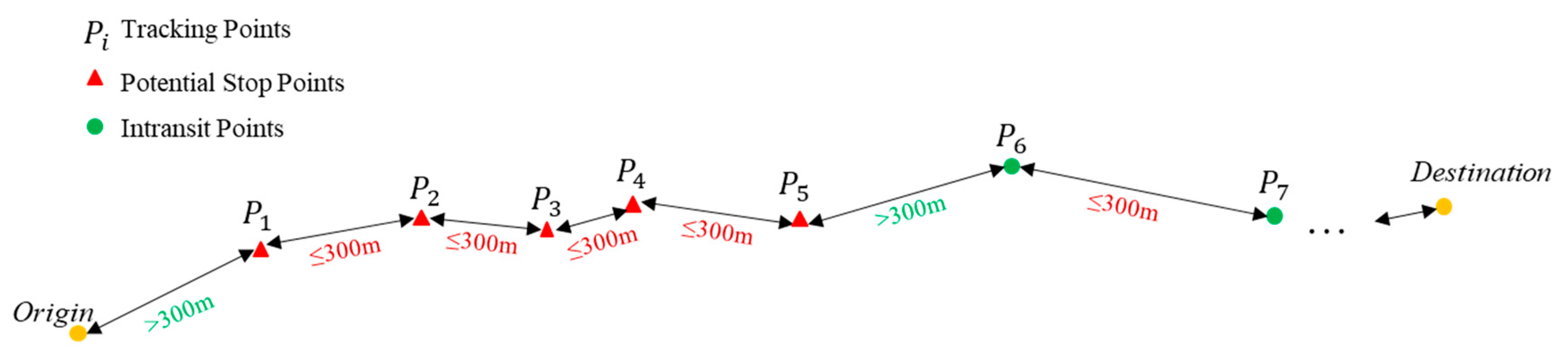
| CounterStops | Number of detected stops. A stop is detected only if at least four data points with a distance below 300 m after each other are detected. | No | T&T |
| Current_DayOfWeek | Day of the current transmission from 1 to 7. | No | T&T |
| Current_DayClass | Day class of current transmission; 1: working day, 2: Saturday or bridge day, 3: Sunday or public holiday. | No | DC |
| Current_Lat and Current_Long | Latitude and longitude of the current transmission. | No | T&T |
| Current_MonthOfYear | Month from 1 to 12 of the current transmission. | No | T&T |
| Current_TimeCategory | Period of the current transmission depending on the desired time interval. For example, a 2-h interval means that there are 12 intervals. | No | T&T |
| Current_TimeInHours | Hour represented as number between 0 to 23.99 of the current transmission. | No | T&T |
| CurrentCountry | Country based on the current position encoded according to ISO-3166 ALPHA-3 (3-letter encoding) using a geo-coder API. | Yes | Coun |
| CurrentGeofenceLocation | ID of the currently identified cluster, otherwise -1. | Yes | Cl |
| DayClassTomorrow | Tomorrow’s day class based current timestamp. | No | DC |
| Departure_DayClass | Departure day class based on the last transmission in the origin; 1: working day, 2: Saturday or bridge day, 3: Sunday or public holiday. | No | DC |
| Departure_DayOfWeek | Departure day from 1 to 7 based on the last transmission in the geo-fence of the origin. | No | T&T |
| Departure_MonthOfYear | Month of departure from 1 to 12 based on the last transmission in the geo-fence of the origin. | No | T&T |
| Departure_TimeCategory | Time of departure based on the last transmission in the geo-fence of the origin and depending on the desired time interval. See also Current_TimeCategory. | No | T&T |
| Departure_TimeInHours | Hour of departure from 0 to 23 based on the last transmission in the geo-fence of the origin. | No | T&T |
| DestinationAbsoluteDistance | Absolute distance in kilometers from the position to the destination. | No | T&T |
| DestinationBearingToPosition | Direction from 0° to 360° from the point of the destination in which the unit load currently is located. | No | T&T |
| DestinationDrivenTime | Time in hours from the current transmission to the destination. Variable to predict. | No | T&T |
| DrivenTimePrevious | Time in hours from the previous transmission to the current transmission. | No | T&T |
| LastGeofenceLocation | ID of the last visited cluster. | Yes | Cl |
| LastRoutePart | Route considering the identified clusters until the current transmission. | Yes | Cl |
| PastActualDistanceToOrigin | Sum of absolute distances between the transmitted positions in kilometers. | No | T&T |
| PastAvgAbsoluteSpeed | Average speed from departure at the origin until the current transmission as a quotient of PastActualDistanceToOrigin and PastDrivenTimeToOrigin. | No | T&T |
| PastDrivenTimeToOrigin | Time in hours from departure at the origin until the current transmission. | No | T&T |
| QuantityDayClass2_nextday5 QuantityDayClass3_nextday5 | Number of Saturdays or bridge days and Sundays or public holidays in the next five days. | No | DC |
| StandingTimeClusterInc | Standing time at the current cluster at a given time. | No | Cl |
| StatusOfRide | Status of current transmission. ‘Origin’ for being at the starting point, ‘Driving’ for being in transport, ‘Stop’ or ‘Destination’ for being at the destination. | Yes | T&T |
| TotalDurationOfStops | Sum of the length of all stops at a given time. | No | T&T |
| TotalLengthOfClusterStop | Sum of the length of all stops at a cluster at a given time. | No | Cl |
| Learning Algorithm | Parameters |
|---|---|
| Support Vector Regression (SVR) | Kernel = ‘rbf’ |
| C = [0.001, 5.001], step size 0.02 | |
| = [0.001, 0.1], evenly split into 30 values | |
| Extremely Randomized Trees (ExtraTrees) | n_estimators = [1, 10], step size 1 |
| random_state = [6, 18], step size 1 | |
| Adaptive Boosting (AdaBoost) | n_estimators = [1, 10], step size 1 |
| learning_rate = [0.0001, 1.0001], step size 0.025 |
| Model | Data Domain | Experiment | MAE | RMSE | Best Parameters |
|---|---|---|---|---|---|
| ExtraTrees | T&T + Day Class + Country + Clustering | Variance threshold 0.9 | 43.66 h | 54.61 h | n_estimators: 12 |
| random_state: 14 | |||||
| AdaBoost | T&T | Variance threshold 0.9 | 18.78 h | 31.00 h | n_estimators: 14 |
| learning_rate: 0.9251 | |||||
| SVR | T&T + Day Class+ Country | ReliefF Top 20 | 16.91 h | 22.70 h | C: 4.801 |
| ε: 0.01 |
| Statistic | SVR | ExtraTrees | AdaBoost | ||||
|---|---|---|---|---|---|---|---|
| Data Domain | MAE | RMSE | MAE | RMSE | MAE | RMSE | |
| T&T data | Average | 31.00 | 38.88 | 108.39 | 119.94 | 103.67 | 113.83 |
| Minimum | 21.87 | 27.49 | 50.27 | 58.91 | 18.78 | 28.40 | |
| Maximum | 47.95 | 56.74 | 125.43 | 134.81 | 119.05 | 131.40 | |
| Standard Dev | 7.59 | 9.09 | 18.07 | 18.50 | 24.70 | 27.21 | |
| T&T data, country and day class | Average | 31.56 | 41.54 | 109.47 | 122.16 | 101.80 | 116.15 |
| Minimum | 16.91 | 22.70 | 63.43 | 75.69 | 19.29 | 30.39 | |
| Maximum | 47.95 | 74.85 | 123.60 | 138.18 | 116.92 | 133.14 | |
| Standard Dev | 8.24 | 13.60 | 14.65 | 14.64 | 24.11 | 25.03 | |
| T&T data, country, day class and clustering | Average | 32.78 | 42.31 | 107.63 | 119.56 | 101.55 | 115.65 |
| Minimum | 18.37 | 25.47 | 43.66 | 54.61 | 19.29 | 32.39 | |
| Maximum | 47.95 | 64.44 | 128.39 | 138.67 | 114.97 | 130.34 | |
| Standard Dev | 8.65 | 11.48 | 20.00 | 20.18 | 23.75 | 24.12 | |
| Over all data domains | Average | 31.78 | 40.91 | 108.50 | 120.55 | 102.34 | 115.21 |
| Minimum | 16.91 | 22.70 | 43.66 | 54.61 | 18.78 | 28.40 | |
| Maximum | 47.95 | 74.85 | 128.39 | 138.67 | 119.05 | 133.14 | |
| Standard Dev | 8.20 | 11.63 | 17.73 | 17.96 | 24.21 | 25.51 | |
© 2019 by the authors. Licensee MDPI, Basel, Switzerland. This article is an open access article distributed under the terms and conditions of the Creative Commons Attribution (CC BY) license (http://creativecommons.org/licenses/by/4.0/).
Share and Cite
Servos, N.; Liu, X.; Teucke, M.; Freitag, M. Travel Time Prediction in a Multimodal Freight Transport Relation Using Machine Learning Algorithms. Logistics 2020, 4, 1. https://doi.org/10.3390/logistics4010001
Servos N, Liu X, Teucke M, Freitag M. Travel Time Prediction in a Multimodal Freight Transport Relation Using Machine Learning Algorithms. Logistics. 2020; 4(1):1. https://doi.org/10.3390/logistics4010001
Chicago/Turabian StyleServos, Nikolaos, Xiaodi Liu, Michael Teucke, and Michael Freitag. 2020. "Travel Time Prediction in a Multimodal Freight Transport Relation Using Machine Learning Algorithms" Logistics 4, no. 1: 1. https://doi.org/10.3390/logistics4010001
APA StyleServos, N., Liu, X., Teucke, M., & Freitag, M. (2020). Travel Time Prediction in a Multimodal Freight Transport Relation Using Machine Learning Algorithms. Logistics, 4(1), 1. https://doi.org/10.3390/logistics4010001