Probability Density Functions for Travel Times in One-Dimensional and Taxicab Service Zones Parameterized by the Maximal Travel Duration of the S/R Machine Within the Zone

Abstract

Travel times for simple trips and cycles are analyzed for a storage/retrieval machine working in a one-dimensional or two-dimensional zone with taxicab geometry. A semi-random trip is defined as one-way travel from a known to a random location or vice versa. A random trip is defined as one-way travel from a random to another random location. The probability density function (PDF) of the travelling time for a semi-random trip in a one-dimensional zone is expressed analytically for all possible locations of its starting point. The PDF of a random trip within the same zone is found as a marginal probability by considering all possible durations for such travel. Then the PDFs for the travel times of single command (SC) and dual command (DC) cycles are obtained by scaling the PDF for the travel time of a semi-random trip (for SC) and as the maximum travel time of two independent semi-random trips (for DC). PDFs for travel times in a two-dimensional service zone with taxicab geometry are calculated by considering the trip as a superposition of two one-dimensional trips. The PDFs for travel times of SC and DC cycles are calculated in the same way. Both the one-dimensional and the two-dimensional service zones are analyzed in the time domain without normalization. The PDFs for all travel times are expressed in an analytical form parameterized by the maximal possible travel time within the zone. The graphs of all PDFs are illustrated by numerical examples.

The subject of this article is to study the probability density functions (PDFs) of travel times for a storage/retrieval (S/R) machine. Knowing the mean and the variance for the travel time is usually enough for the analysis of many warehouse processes such as order picking. Such an approach was demonstrated in the 1970s and is still applied in recent research; thus, the PDFs are generally overlooked. For this reason, the present study aims to obtain the analytical form of PDFs for the travel times of basic trips and storage/retrieval cycles, to summarize and illustrate them in a few pages. Once the PDF is presented in an analytical form, the expected mean travel time can be also expressed analytically and checked against previously published results.

1. Introduction and Motivation

Supply chain management (SCM) heavily relies on automation at every node—production, transportation, distribution, retail, etc. The performance of each SCM node depends on the machines used, especially within the warehouse. Nowadays, the typical warehouse is changed by the emergence of new digital industrial technology, known as Industry 4.0. The Internet of Things (IoT) and cloud computing can make warehouse processes more agile [1]. However, better decision-making can occur if the underlying processes are known. Such a requirement has already been identified for optimizing the processes in transportation, which motivates the analysis of the travel time distribution for these systems [2].

Similarly, to maximize the positive impact of Industry 4.0 on the automated storage and retrieval systems (AS/RS) typically used within SCM, a good understanding of travel times with a stochastic nature is required. The aim of this paper is to analyze and define the analytical form of probability density functions for the travel times of different trips and cycles in simple models of warehouse logistics. Namely, a one-dimensional service zone and a two-dimensional service zone with taxicab geometry will be considered.

AS/RS have been a subject of analysis since the mid-20th century, and many papers have been published on the topic. A survey of the literature [3] is therefore a good start for any new analysis in this field.

The first analyses of travel time models for AS/RS were published in the 1960s by [4] and [5]. In the 1970s, several authors worked on travel time models considering various rack shapes, with a special focus on square-in-time racks. One of them, Gudehus, published a series of works on travel times [6,7,8] for AS/RS. Along with the paper by Bozer and White [9], Gudehus’ works are often referenced as fundamental travel time models, even by research published recently [10]. What is common in these models is that they apply a normalized time domain for the service zone.

From the survey [3], one can see that over the years, studies of expected travel times (in two- and three-dimensional spaces) have implicitly used the one-dimensional model as part of more complex problems. Because the subject of the studies always varies, the authors only calculate the probability characteristics of the one-dimensional movement required for their calculations. Examples of this approach for an implicit interest in the stochastic properties of one-dimensional travel are [11] and [12]. Over the years, this research has followed the same equations developed by Gudehus, although their form may slightly differ. Some of his own recent works demonstrate a lack of further development of said models. For example, in [13], one can see that the approach to the probability characteristics of the one-dimensional trips is not much different.

Vickson and Lu’s work [14] deserves attention; it is dedicated to one-dimensional storage racks. In this work, the authors approach several problems in a one-dimensional discrete model. As the present work applies a continuous model, it shall be noted that continuous modelling is applicable for one-dimensional discrete models even with a relatively low number of discrete states. A study [15] reported that applying a continuous model to a rack with nine discrete addresses (bins) leads to less than 1% deviation in the calculated characteristics of the travel times.

However, an important reason to run an in-depth analysis of the one-dimensional model is that it can be considered as an element of more sophisticated service models. When the probability density function (PDF) of the travel time for trips in a one-dimensional model is known, it can then be applied to other, more sophisticated spatial queueing models. A study in 2006 [16] defined a method by which the PDF for travel times can be determined when the S/R station is located in a corner of the service zone. Later, in [17], this method was further developed to calculate the PDFs for travel times from any point within the zone.

Last, but not least, a dedicated analysis of the PDF of travel times is needed because it is a powerful instrument for calculating any stochastic characteristics, such as mean and variance. By knowing the PDF of the travel time, all its moments can be calculated. Still, studies usually focus on performance, throughput, optimization, or another topic of improvement, while the PDFs are pushed aside. A good example is the work [18] in which an approximation of the PDF for dual command travel time is published and is still noted as a by-product of the research.

2. Semi-Random and Random Trips

This section analyzes basic trips for a mobile server in one-dimensional zone services. This model may represent an elevator in a tall building or the travelling of a forklift in a single corridor between shelves. Let us consider any two locations A and B within the zone; we assume that the travelling time from A to B equals the travelling time from B to A. Then, we define the following basic trips:

• Random trip—travelling between two random locations within the zone, where both locations are independent of each other and uniformly distributed.
• Semi-random trip—travelling between an arbitrary, yet known location and a random location uniformly distributed. As the travelling times from A to B and from B to A are the same, we can disregard whether the start or the end location is a random one.

The objective is to find the probability density functions for the travel times of the above trips.

2.1. Model Definition

A one-dimensional horizontal service zone is considered with length L which is serviced by a mobile device (server) with well-known characteristics (velocity, acceleration times, etc.). Let the maximal duration for a single trip of the server within the zone be T, which applies for the maximal possible distance L. Service requests appear within the zone at uniformly distributed random locations. Let τ be a continuous random variable equal to the travel duration of the server to the next service request. The question is as follows: what is the probability density function of τ?

The initial case to be considered is a semi-random trip for the server; i.e., it will start its route from an arbitrary (known) location K to the random location where the service request appears. Let us denote the travel time ${\tau }_K$ and its PDF $f\left({\tau }_K\right)=f_K\left(t\right)$.

As the server characteristics are known, its travelling within the service zone will only be considered in the time domain, i.e., the travel duration is measured rather than the travel distance. A coordinate system is defined with an origin point O at the left end of the horizontal area. The coordinates of the server and the request in the so-defined time domain will represent the time required to travel to them from the origin. Hence, the coordinate k of the known location K is defined as $k=\left[0,T\right]$, and it represents the travel duration from O to the known location K.

2.2. Model Limitations

While the analysis is focused on the travelling times of an S/R machine, there are several simplifications made. These simplifications prevent the direct applicability of the model and shall be addressed when calculating travel and service times in real scenarios. These limitations include the following:

• The velocity of the S/R machine is considered to be constant. Fluctuations caused by load, downtimes, or external factors are ignored;
• Acceleration and deceleration times of the S/R machine are ignored;
• Storage and retrieval times are ignored, and the S/R machine is considered to depart from a given location immediately after arrival.

Such simplifications of the model are not unusual (e.g., they are also applied in [9]). The limitations caused by them can be addressed by the principle of superposition when their impact on the travel times is known.

Furthermore, the model assumes a random storage strategy. Storage and retrieval requests appear for random locations uniformly distributed within the entire service zone. Whenever an ABC or another zone-based storage strategy is applied, the model shall be adapted as the PDFs will be different.

The same limitations apply for the two-dimensional service zone considered in Section 4.

2.3. Semi-Random Trip

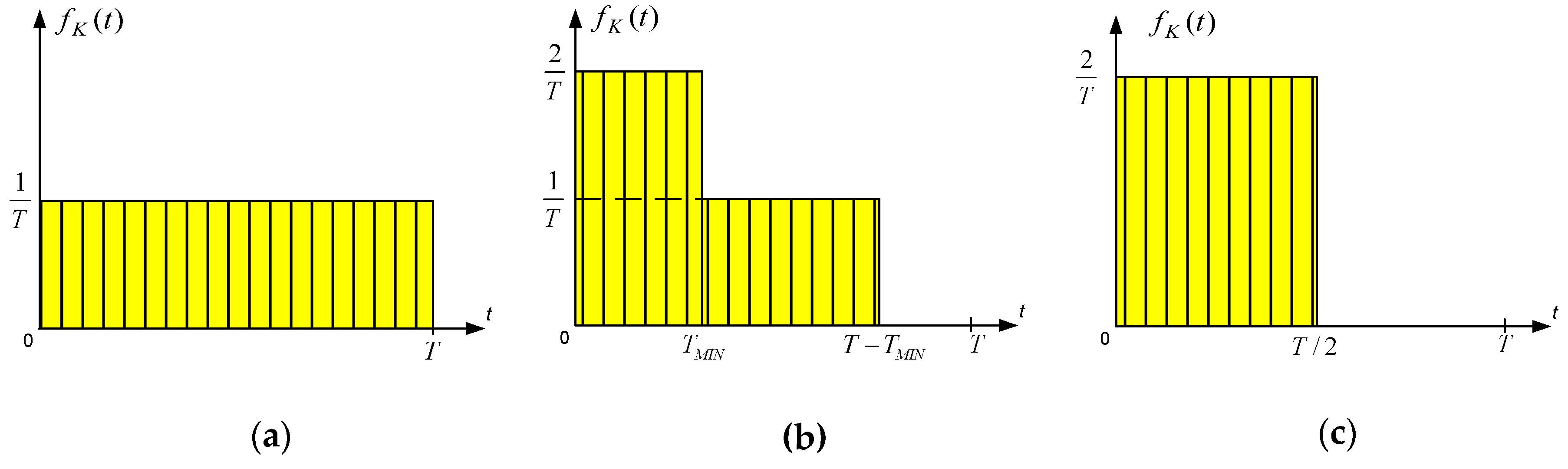
The duration τ of the travel from K to a random point within the zone is $\tau =\left[0,T\right]$. Without doubt, $f_K\left(\tau \right)$ will depend on the distances from K to both ends of the service zone, as these distances limit the trip. If T_MIN is the travel duration from K to the nearer end of the zone, i.e., $T_{MIN}=Min\left\{k,T-k\right\}$, then the probability density of the semi-random trip duration can be written

$$f\left({\tau }_K\right)=f_K\left(t\right)=\{\begin{array}{cc}2/T& 0\le t\le T_{MIN}\\ 1/T& T_{MIN}<t\le T-T_{MIN}\\ 0& T-T_{MIN}<t\le T\\ 0& otherwise.\end{array}$$

(1)

This PDF consists of two intervals, both of which have a constant value, and the value within the second interval is half of the value in the first one, as illustrated in Figure 1b. In the boundary cases $k=0$ and $k=T/2$ (shown in Figure 1a,c), the corresponding functions $f_K\left(t\right)$ are uniformly distributed in the intervals $\left[0\dots T\right]$ and $\left[0\dots T/2\right]$, respectively. The boundary case $k=0$ also represents the PDF of travel duration to a random point when the server is located at the end of the zone. Obviously, in the case where $k=0$ the mean of the travel duration is $E_K\left(\tau \right)={{\displaystyle \int }}_0^T\mathsf{\tau }{f}_K\left(\mathsf{\tau }\right)d\mathsf{\tau }=T/2$, as published already in the first work by Gudehus [6].

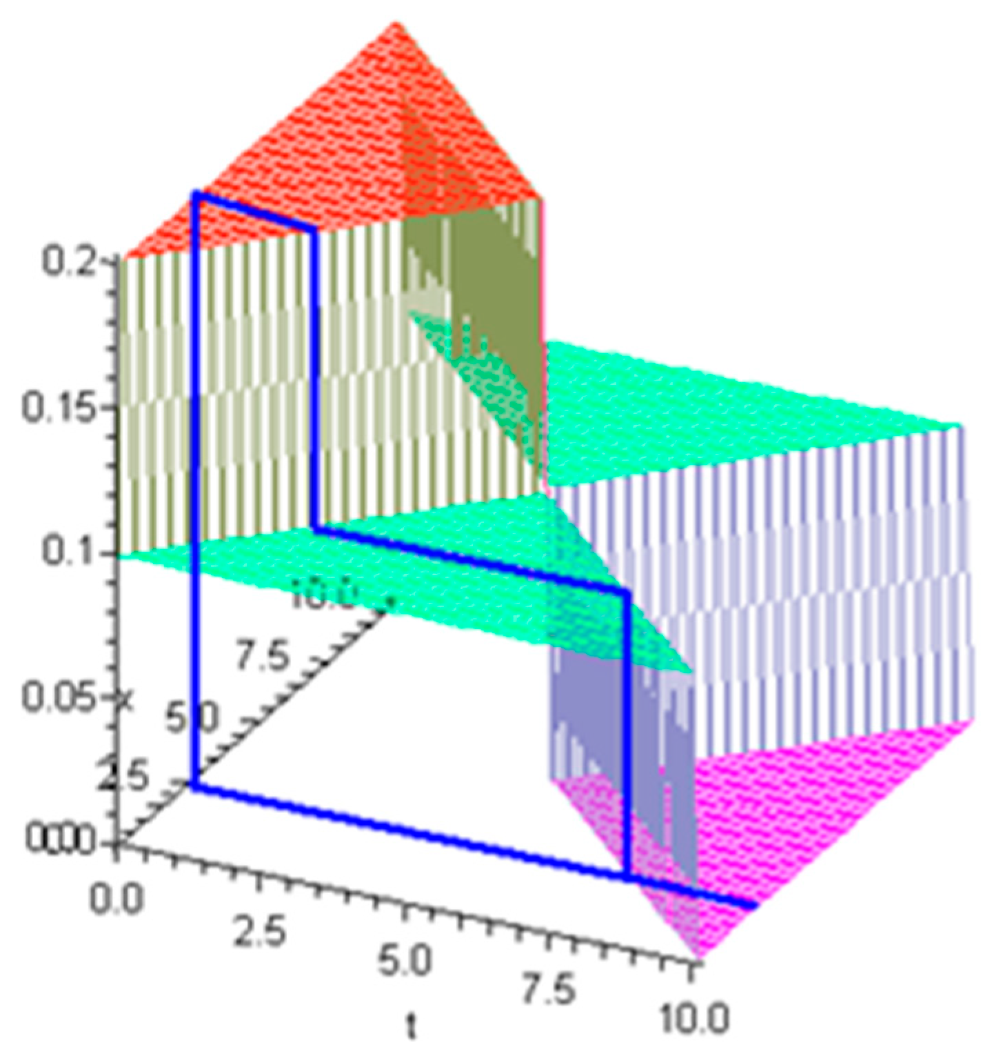
However, how does the PDF $f_K\left(t\right)$ change for other values of k? As k is a continuous variable, it is possible to calculate and visualize $f_K\left(t\right)$ for any point K within the service zone. We will visualize all values of k in a single graphic. To do this, a third axis will be added to the graphic in Figure 1b, which will indicate the value of k for which the PDF $f_K\left(t\right)$ is calculated. This is illustrated in Figure 2, where the value of k is indicated on axis x and τ on axis t. The graph is generated for a service zone with length $L=10 m$ and server velocity $v=1 m/s$; hence, $T=10 s$. Acceleration times are ignored.

2.4. Random Trip

The graphic in Figure 2 is quite interesting. Each 2D section of it normal to axis x represents the graph of $f_K\left(\tau \right)$, which is the density of the conditional probability $P_K\left(\tau \right)=P(\tau \le t|k)$ for the given value of k. In other words, the 2D section emphasized in Figure 2 is the graph of the PDF for the duration τ of a semi-random trip of the server to a random request to be not greater than t when the server is located at known point K. Obviously the value of k is the point of incidence of the 2D section with the x axis.

Let us now consider the server location K to be unknown and its coordinate $\xi =\left[0\dots T\right]$ to denote the duration of a semi-random trip from O to the unknown K. Let $k=\left[0\dots T\right]$ be a parameter denoting a specific location, and let the probability $\mathrm{Pr}\left(\xi \to k\right)$ be uniformly distributed.

As $f_K\left(t\right)$ represents a PDF of conditional probability, then it could be written

$$\mathrm{Pr}\left(\xi \to k\cap \tau \to t\right)\iff f\left(\tau ,\xi \right)=f\left(\xi \right)f_K\left(t\right)$$

(2)

where $f\left(\tau ,\xi \right)$ is the joint PDF of the two dependent random variables τ and ξ. As any value of k is equally probable, the PDF of $\xi$ is $f\left(\xi \right)=1/T$. Having this in mind, by multiplying the vertical axis in Figure 2 by $1/T$ the resulting graph will represent the joint mass function $f\left(\tau ,\xi \right)$ (Figure 3). Every point on this graph gives the value of the joint PDF for the simultaneous occurrence of both random events: (A) the travel duration to the next request is in the epsilon neighborhood of time t, and (B) the server is located in the epsilon neighborhood of k. The graph represents all possible values of the variables τ and ξ.

Now let us consider a section normal to axis t on the graph of Figure 3 with point of incidence $t$. The surface $s\left(t\right)$ of this section is an integral sum on all possible values of ξ for $\tau \to t$, and the following could be written for it:

$$s\left(t\right)=\underset{0}{\overset{T}{{\displaystyle \int }}}f\left(\tau ,\xi \right)d\xi =\underset{-\infty }{\overset{+\infty }{{\displaystyle \int }}}f\left(\tau ,\xi \right)d\xi =f\left(\tau \right).$$

(3)

What is important in Equation (3) is that the exact location of the server is disregarded by taking into account all its possible locations. Thus, the function $f\left(\tau \right)$ is a marginal probability density function for the duration of travel from a random to random location in the 1D service area (i.e., for a random trip).

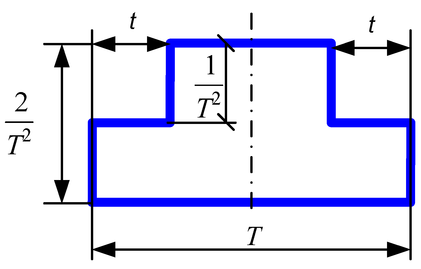
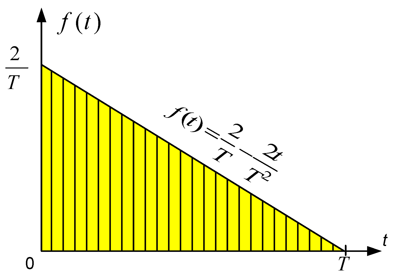
By geometrical considerations of the section clarified in Figure 4, the PDF can be calculated as

$$f\left(\tau \right)=s\left(t\right)=\frac{2}{T}-\frac{2t}{T^2} .$$

(4)

The PDF graph is illustrated in Figure 5. It is a ramp function with negative slope. For this distribution, the expected mean value is $E\left(\tau \right)={{\displaystyle \int }}_0^T\tau f\left(\tau \right)d\tau =T/3$, i.e., the mean value of the random trip duration is one-third of the maximum possible travel duration within the area. This value was also published by Gudehus in [7], and it was used later by many authors for various calculations.

Equations (1) and (4) define the PDF for the basic semi-random and random trips. On their basis, we can further calculate the travel times for different trips and service cycles of the mobile server in a one-dimensional or a two-dimensional service zone with taxicab geometry.

3. One-Dimensional Zone with an S/R Station at the End

We consider a one-dimensional service zone with maximal travel time T across it, as defined in the previous section. However, we will add to the model a storage/retrieval (S/R) station located at one of its ends (for instance, at the left end of the zone). The probability density functions for the travel times of single command and dual command cycles shall be defined.

It should be noted that the random trip by definition is a trip between two random locations, and consequently, its travel time is independent of the location of the S/R station. Hence, its PDF $f\left(\tau \right)$ is defined by Equation (4) and does not require further analysis.

3.1. Single Command Cycle

The single command (SC) cycle is a travelling cycle of the mobile server for servicing a single request (single command). This could be a storage request or a retrieval request. In either case, the server location is assumed to be the S/R station at the beginning of the cycle. A storage request cycle will start with loading at the S/R station; the server travelling to a random location where the load shall be stored; storing the request; and a return of the empty server back to the S/R station to close the cycle. A retrieval request cycle will start with the empty server travelling to a random location; loading at this location; travelling back to the S/R station; and unloading.

For the 1D model defined we can define the travel time for a semi-random trip starting from or ending at the S/R station as a random variable ${\tau }_K$ in the domain $\left[0,T\right]$. Then, considering Equation (1) as its PDF, we can write

$$f\left({\tau }_K\right)=f_K\left(t\right)=\{\begin{array}{cc}1/T& 0\le t\le T\\ 0& otherwise.\end{array}$$

(5)

Knowing the PDF of the semi-random trip duration ${\tau }_K$, one can easily calculate the PDF for the duration ${\tau }_{SC}$ of a single command cycle. The SC cycle consists of two identical semi-random trips—from the S/R station to a random location and back from the same location to the S/R station. Hence, it is a random variable ${\tau }_{SC}=2{\tau }_K$, defined in the domain $\left[0,2T\right]$. Its PDF $f\left({\tau }_{SC}\right)$ has a similar form as $f\left({\tau }_K\right)$; however, it is stretched horizontally and compressed vertically by a factor of 2:

$$f\left({\tau }_{SC}\right)=f_{SC}\left(t\right)=\frac{1}{2}{f}_K\left(\frac{1}{2}t\right)=\{\begin{array}{cc}1/2T& 0\le t\le 2T\\ 0& otherwise.\end{array}$$

(6)

3.2. Dual Command Cycle

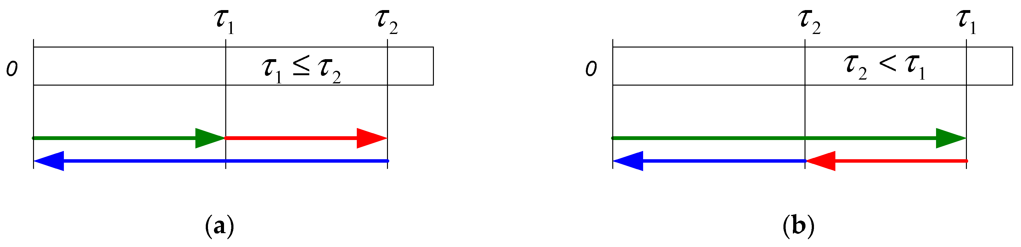
The dual command (DC) cycle combines serving both a storage and a retrieval request. It starts with loading at the S/R station; the server travelling to a random location for storage; unloading; the empty server travelling to a location for retrieval; loading; travelling to the S/R station; and unloading.

Let us consider a dual command cycle within the same 1D service zone, where the storage/retrieval station is located at the origin O. Every dual command cycle begins and ends at the origin O. If ${\tau }_1$ denotes the duration of a semi-random trip from O to an unknown storage location and ${\tau }_2$ denotes the duration of a semi-random trip from the retrieval location to O, then for the duration of the dual command cycle ${\tau }_{DC}$ there are two cases possible, as visualized in Figure 6.

In the first case (Figure 6a) the storage location is closer to point O, i.e., the duration of the dual command cycle consists of travelling ${\tau }_1$; then time for travelling further to the retrieval location; and, finally, the travelling time ${\tau }_2$ back to the origin O. Hence, the travelling time between the random locations for storage and retrieval equals the difference ${\tau }_2-{\tau }_1$. Therefore, the total duration of the dual command cycle amounts to ${\tau }_{DC}=2{\tau }_2$ in the domain $\left[0,2T\right]$. In the second case (Figure 6b), following the same logic, the total duration of the DC cycle will be ${\tau }_{DC}=2{\tau }_1$, as the retrieval point resides on the way back from the storage location to point O. The two cases could be summarized as

$${\tau }_{DC}=2max\left({\tau }_1,{\tau }_2\right)=2{\tau }_{MAX}.$$

(7)

However, ${\tau }_1$ and ${\tau }_2$ are two independent and identically distributed random variables of travel time for a semi-random trip with PDF defined in Equation (5). Their maximum ${\tau }_{MAX}=max\left({\tau }_1,{\tau }_2\right)$ is known to have the PDF

$$f\left({\tau }_{MAX}\right)=\{\begin{array}{cc}2{\tau }_{MAX}/T^2& 0\le {\tau }_{MAX}\le T\\ 0& otherwise.\end{array}$$

(8)

(This PDF is also the one for travel time from a corner point to a random location in the Single-In-Time (SIT) Tchebyshev’s metric, where the travel times on the different axes are independent and identically distributed (see [16]).)

Hence, the PDF for the travel duration of a dual command cycle travel is a ramp function in the interval $\left[0\dots 2T\right]$, and the analytical form of this PDF is

$$f\left({\tau }_{DC}\right)=f_{DC}\left(t\right)=\{\begin{array}{cc}\frac{t}{2T^2}& 0\le t\le 2T\\ 0& otherwise.\end{array}$$

(9)

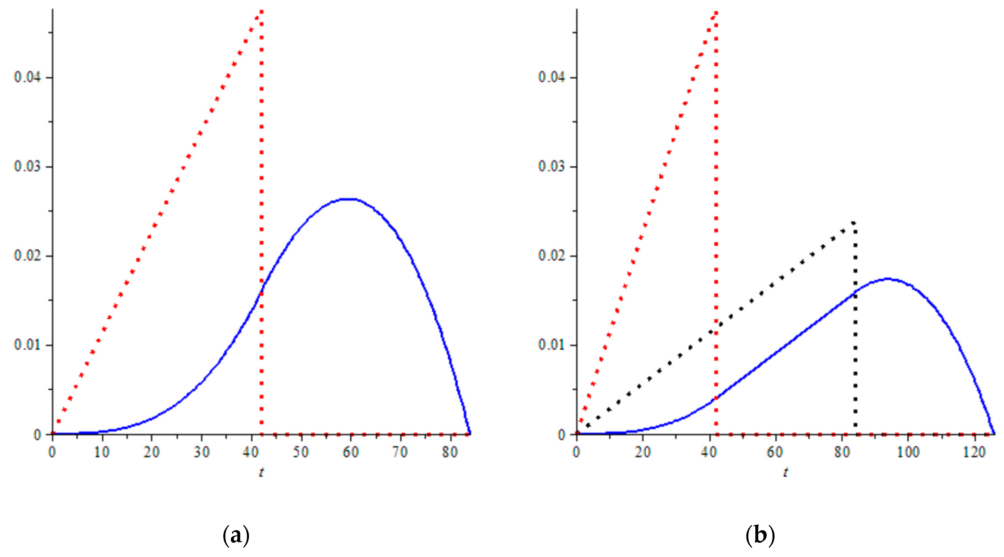
In Figure 7 are visualized the graphs of the probability density functions for the different travel times in a one-dimensional service zone with an S/R station at its end and maximal travel time $T=42s$. A semi-random trip from the S/R station (cyan dashed), a random trip between two random locations within the zone (magenta dashed), an SC cycle (green solid), and a DC cycle (blue solid) are shown.

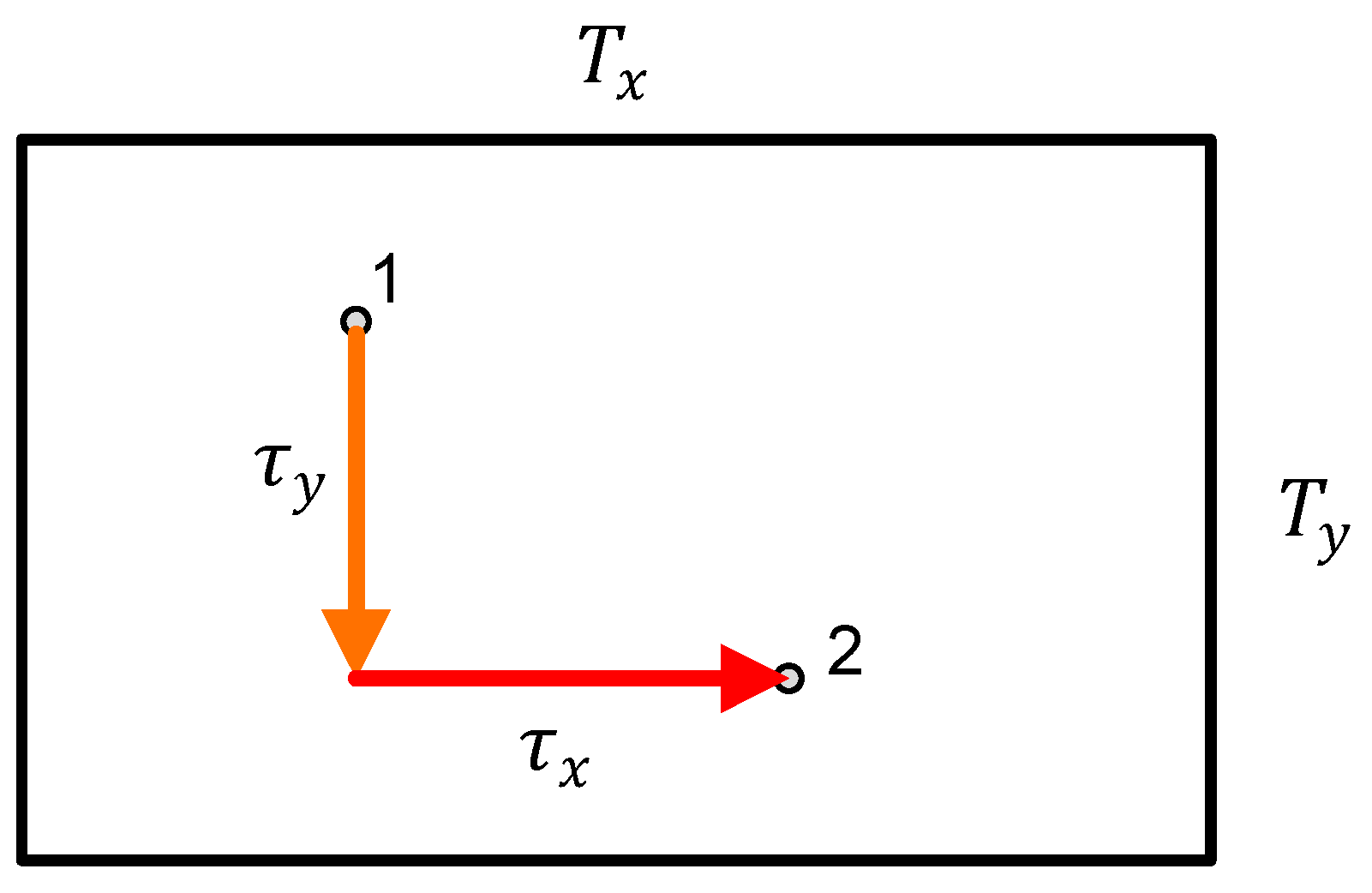
4. Two-Dimensional Zone with Taxicab Geometry

We consider a rectangular service zone with size $L\times H$, in which service requests may appear uniformly distributed anywhere within the zone. Let us assume that the zone is served by a mobile server travelling only in directions parallel to the rectangle sides—it can travel in a direction either parallel to the long side or parallel to the short side. It cannot travel simultaneously in both directions. Such a model may represent the travelling of a forklift within a warehouse or a cab through a city with orthogonal streets. The distance measurement in this setup is known as the Manhattan metric, and it equals the sum of the distance travelled in each direction.

Let the server travel with velocity $v_x$ along the side with length L and with velocity $v_y$ along the side with length H. Then the maximal times for travelling in the corresponding directions are $T_x=L/v_x$ (direction X) and $T_y=H/v_y$ (direction Y). The maximal total travel time for a single trip within the zone is then $T=T_x+T_y$. The model setup in the time domain is presented in Figure 8, where the service zone has size $T_x$ on $T_y$.

These maximal travel times $T_x$ and $T_y$ will be used as parameters for the definition of the PDFs for the different random travel times, i.e., all equations will be made in the time domain without normalization by using a “shape factor” as suggested in [9]. Without loss of generality, it will be assumed that $T_x\ge T_y$.

The travel time for a random trip from Point 1 to Point 2 shown in Figure 8 will be equal to the sum of the travelling duration in both directions, ${\tau }_x+{\tau }_y$, as the server will first travel ${\tau }_y$ seconds in one direction and then ${\tau }_x$ seconds in the other direction (Equation (10)). This equation defines the property of the server to move only in one direction at any given time, and hereafter it will be referred to as the “taxicab property”. The travel time domains are defined by the maximal travel times: ${\tau }_x\in \left[0,T_x\right]$, ${\tau }_y\in \left[0,T_y\right]$, and ${\tau }_{1\to 2}\in \left[0,T\right]$.

$${\tau }_{1\to 2}={\tau }_x+{\tau }_y$$

(10)

Let the storage/retrieval (S/R) station be located in one of the four corners of this service zone (for instance, in the lower left corner). A single command cycle will then be defined as a semi-random trip from the S/R station to a random point within the zone, followed by a return to the S/R station (i.e., the SC is a doubled semi-random trip). A dual command cycle will be defined as a semi-random trip from the S/R station to a random Location 1; followed by a random trip to Location 2; followed by a semi-random trip from Location 2 back to the S/R station.

The objective is to find the PDF of the travel time for the basic semi-random and random trips, as well as for the two cycles. To achieve this objective, the taxicab property will be used.

4.1. Semi-Random Trip and Single Command Cycle

In this section, we will find the density function of the travel time ${\tau }_K$ for a semi-random trip, as well as the travel time ${\tau }_{SC}$ for an SC cycle in the 2D zone.

Due to the taxicab property, the travelling times in both directions can be considered as independent random variables and the total travel time as a sum of independent (one-dimensional) random variables. This sum is well known from probability theory, and its PDF is defined as a convolution of the PDFs of the two independent random variables. Let ${\tau }_{Kx}$ and ${\tau }_{Ky}$ denote the travel times for a semi-random trip from the S/R station to a random location in direction X and direction Y correspondingly.

The PDFs for the travel times ${\tau }_{Kx}$ and ${\tau }_{Ky}$ are PDFs of one-dimensional semi-random trips, and considering the PDF in Equation (5), one can write Equations (11) and (12).

$$f\left({\tau }_{Kx}\right)=f_{Kx}\left(t\right)=\{\begin{array}{cc}1/T_x& 0\le t\le T_x\\ 0& otherwise\end{array}$$

(11)

$$f\left({\tau }_{Ky}\right)=f_{Ky}\left(t\right)=\{\begin{array}{cc}1/T_y& 0\le t\le T_y\\ 0& otherwise\end{array}$$

(12)

The PDF of ${\tau }_K$ is then defined as the convolution of the travel times in directions X and Y (with $T=T_x+T_y$ and assuming $T_x\ge T_y$):

$$f\left({\tau }_K\right)=f_K\left(t\right)=f_{Kx}\left(t\right)\ast f_{Ky}\left(t\right)=\{\begin{array}{cc}\frac{t}{T_x{T}_y}& 0\le t\le T_y\\ \frac{1}{T_x}& T_y<t\le T_x\\ \frac{T-t}{T_x{T}_y}& T_x<t\le T\\ 0& otherwise.\end{array}$$

(12)

Further, as the SC cycle is a doubled semi-random trip, its PDF can be obtained as the PDF defined in Equation (13) stretched horizontally and compressed vertically by a factor of 2:

$$f\left({\tau }_{SC}\right)=f_{SC}\left(t\right)=\frac{1}{2}{f}_K\left(\frac{1}{2}t\right)=\{\begin{array}{cc}\frac{t}{4T_x{T}_y}& 0\le t\le 2T_y\\ \frac{1}{2T_x}& 2T_y<t\le 2T_x\\ \frac{T-\frac{t}{2}}{2T_x{T}_y}& 2T_x<t\le 2T\\ 0& otherwise.\end{array}$$

(13)

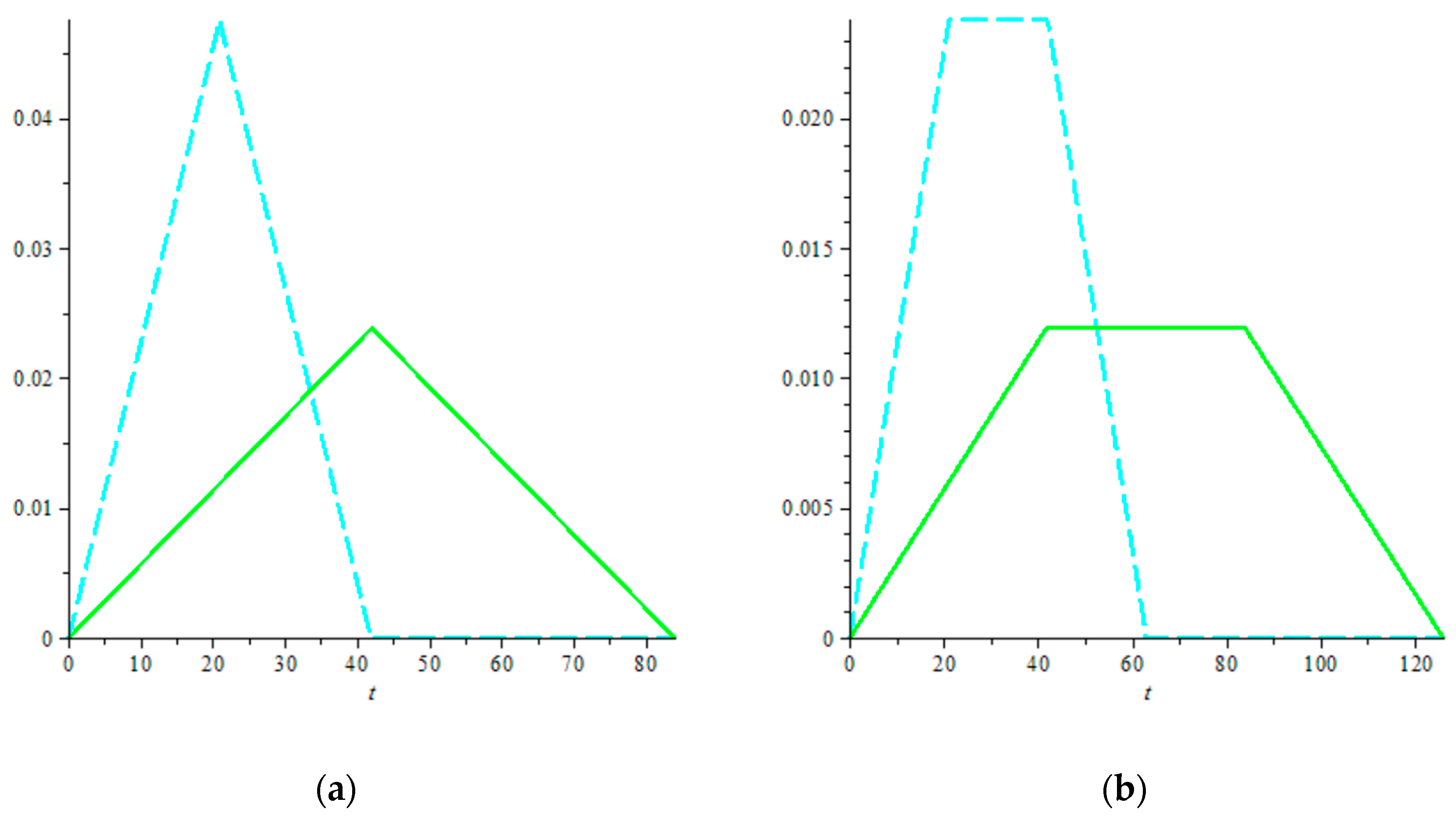
To illustrate the nature of the PDFs $f_K\left(t\right)$ and $f_{SC}\left(t\right)$, their graphs are shown in Figure 9 for two sample cases: $T_x=T_y=21 seconds$ (square-in-time zone) and $T_x=2T_y=42 seconds$.

Here a reference could be made to [16], where the PDF for the travel time from a corner to a random location in a service zone with the Manhattan metric was calculated on the basis of isochrones. It was demonstrated that the PDF has the form of an isosceles trapezoid (or triangle for a square-in-time zone). However, in that article the equations were made for a normalized time domain by using a shape factor for normalization. The approach described in the present work has the advantage of defining the PDFs of the travel times without normalization; hence, the moments of the random variables can be calculated directly without the need for denormalization.

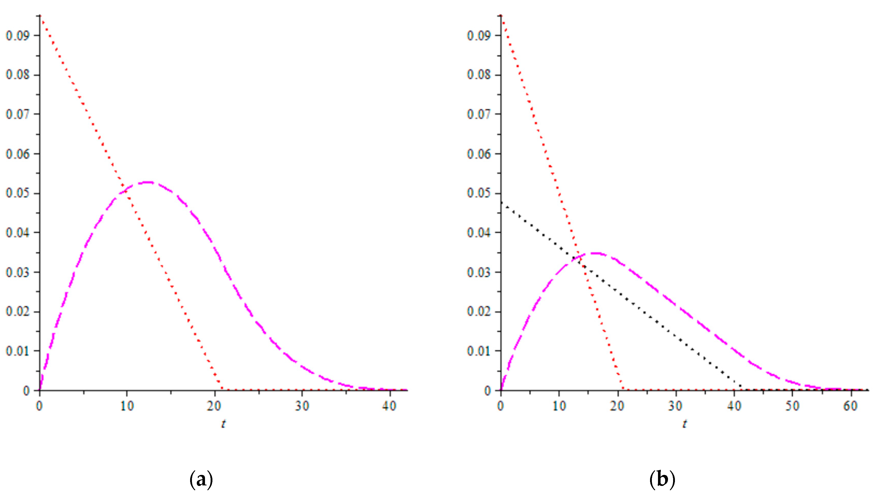
4.2. Random Trip

In this section, we will find the density function of the travel time $\tau$ for a random trip. Using the taxicab property of the model again, $\tau$ can be considered as a sum of two independent one-dimensional random variables ${\tau }_x$ and ${\tau }_y$, being the travel times for the random trip in direction X and direction Y.

The PDFs for the travel times ${\tau }_x$ and ${\tau }_y$ are PDFs of one-dimensional random trips, and considering the PDF in Equation (4), one can write Equations (15) and (16).

$$f\left({\tau }_x\right)=f_x\left(t\right)=\{\begin{array}{cc}\frac{2}{T_x}-\frac{2t}{T_x{}^2}& 0\le t\le T_x\\ 0& otherwise\end{array}$$

(14)

$$f\left({\tau }_y\right)=f_y\left(t\right)=\{\begin{array}{cc}\frac{2}{T_y}-\frac{2t}{T_y{}^2}& 0\le t\le T_y\\ 0& otherwise\end{array}$$

(15)

The PDF of $\tau$ is then defined as the convolution of the travel times in directions X and Y (with $T=T_x+T_y$ and assuming $T_x\ge T_y$):

$$f\left(\tau \right)=f\left(t\right)=f_x\left(t\right)\ast f_y\left(t\right)=\{\begin{array}{cc}\frac{4t}{T_x{T}_y}\left(1-\frac{Tt}{2T_x{T}_y}+\frac{t^2}{6T_x{T}_y}\right)& 0\le t\le T_y\\ \frac{2}{T_x{}^2}\left(T_x-t+\frac{T_y}{3}\right)& T_y<t\le T_x\\ \frac{2}{3T_x{}^2{T}_y{}^2}{\left(T-t\right)}^3& T_x<t\le T\\ 0& otherwise.\end{array}$$

(16)

To illustrate the nature of the above PDFs $f_x\left(t\right)$, $f_y\left(t\right)$, and $f\left(t\right)$, their graphs are shown in Figure 10 for two sample cases: $T_x=T_y=21 seconds$ (square-in-time zone) and $T_x=2T_y=42 seconds$.

4.3. Dual Command Cycle

Further, for the DC cycle we apply the same approach. Using the taxicab property we can define the total travel time ${\tau }_{DC}$ for a DC cycle as a sum of two independent DC cycles in direction X and direction Y. Applying Equation (9) for each direction, we can write:

$$f\left({\tau }_{DCx}\right)=f_{DCx}\left(t\right)=\{\begin{array}{cc}\frac{t}{2T_x{}^2}& 0\le t\le T_x\\ 0& otherwise\end{array}$$

(17)

$$f\left({\tau }_{DCy}\right)=f_{DCy}\left(t\right)=\{\begin{array}{cc}\frac{t}{2T_y{}^2}& 0\le t\le T_y\\ 0& otherwise.\end{array}$$

(18)

The PDF of ${\tau }_{DC}$ is then defined as the convolution of the travel times in directions X and Y (with $T=T_x+T_y$ and assuming $T_x\ge T_y$):

$$f\left({\tau }_{DC}\right)=f_{DC}\left(t\right)=f_{DCx}\left(t\right)\ast f_{DCy}\left(t\right)=\{\begin{array}{cc}\frac{t^3}{24T_x{}^2{T}_y{}^2}& 0\le t\le 2T_y\\ \frac{3t-4T_y}{6T_x{}^2}& 2T_y<t\le 2T_x\\ \frac{2T-t}{24T_x{T}_y}\left(t^2+2Tt-8\left(T_x{}^2+T_y{}^2-T_x{T}_y\right)\right)& 2T_x<t\le 2T\\ 0& otherwise.\end{array}$$

(19)

An illustration of the above PDFs $f_{DCx}\left(t\right)$, $f_{DCy}\left(t\right)$, and $f_{DC}\left(t\right)$ is shown in Figure 11 for the two sample cases: $T_x=T_y=21 seconds$ (square-in-time zone) and $T_x=2T_y=42 seconds$.

Side note: It could be interesting to make a quick reference here to the approximation suggested by Foley and Frazelle in their work [18] for the PDF of DC travel time (although they analyzed a discrete model, they turned to continuous modelling for calculating this PDF). They analyzed an AS/RS working in Tchebyshev’s metric, and the present model analyzes an S/R machine working in taxicab geometry. For this reason the PDF for the DC travel time suggested by them cannot be directly compared with the PDF suggested here. What is, however, remarkable is that there are similarities in the form of the PDF graph they illustrated (Figure 3 in their work) and the graph illustrated in Figure 11a here. Comparing Equation (17) in the present work with their Equation (5) explains these similarities—when integrated (to obtain a cumulative distribution function), Equation (17) above will become a term of the fourth power of the random variable in its first subdomain and a polynomial of degree four in its third subdomain. 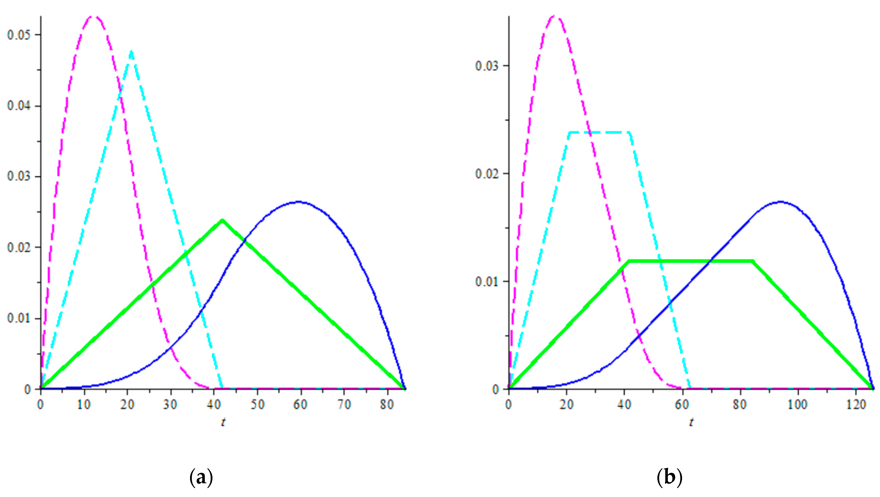End of side note.

The probability density functions defined in this section for the travel times of basic trips and SC and DC cycles were illustrated in different domains. For a better overview on how they scale to each other, their graphs are illustrated again in Figure 12 within the same domain.

As the probability density functions of the travel times are now defined in analytical form, their moments can be used for the calculation of different random variables—the expected average travel time, expected variance, or standard deviation, etc., from each corresponding PDF.

5. Conclusions

This study demonstrated how the probability density functions for travel durations can be developed for a service zone with a known geometry and the properties of the S/R machine serving it. Starting with the PDFs for simple trips, the PDFs for more sophisticated travels were obtained through well-known mathematical dependencies as functional transformations or convolution. The PDFs developed in this paper can be used to further express travel times for other cycles in one-dimensional or two-dimensional service zones. The illustration of their graphs summarized in Figure 7 and Figure 12 may help students and newcomers to AS/RS analysis to better understand the processes.

The suggested approach does not require normalization of the service zone, and all PDFs are defined in the time domain. Hence, random variables calculated on their basis will not require denormalization. For instance, the mean value $E\left(\tau \right)$ will be obtained in seconds. In contrast, the classical approach by Bozer and White [9] uses normalization via a shape factor of the service zone geometry, and it requires denormalization of the results. Another advantage of the approach without normalization is that the PDFs of the travel times can be parameterized by the maximal travel times in the service zone. This can facilitate the development of Information Technology applications in the field of warehouse logistics and SCM. For instance, the travel times in two warehouses with the same geometry, but serviced by S/R machines with different velocities, will have identical analytical forms. Their numerical values will, however, differ due to the different travel times of the S/R machines.

The simplifications pointed out in Section 2.2. could serve as a starting point for further studies. A few examples are demonstrating the impact of acceleration and deceleration times on the PDFs of the travel times; or analyzing the proportion of the time for travelling and the time for storage/retrieval out of the total service time; or how the PDFs for travel times will look when a zone-based storage strategy is applied in a warehouse.

Future research can also develop the PDFs for travel times in Tchebyshev’s metric, which is of special interest for warehouse processes. The side note in Section 4.3 above could be a starting point for such analysis, where the objective would be to develop the analytical form of the PDF for DC travel time and compare it with the approximation suggested in [18].

Last, but not least, knowing the PDFs for travel and service times in a given model immediately defines the distribution G of service times for requests if the model is considered as an M/G/1 queue. This opens the door to analysis of more sophisticated models. For instance, a warehouse with well-defined geometry and properties of its S/R machines could be represented as a queueing network, where each S/R machine will be a queue with a known service time distribution G.