Abstract
When preserving perishable goods, maintaining a constant temperature over the cold supply chain is essential. Therefore, refrigerated vehicles are an important part of the cold supply chain system. However, many traditional refrigerated cargo systems are not designed to support the homogeneity of the temperature inside cargo trailers. Indeed, refrigerating equipment is usually placed on one side of transportation systems as this is considered to be more practical. Such a configuration thus leads to significant temperature differences in the two distinct parts of a refrigerated cargo trailer, which might affect the quality, safety, and shelf life of perishable foods. This research aims to improve the temperature distribution of refrigerated trailers. In this study, it is highlighted that in the most commonly used traditional refrigerated trailer models, lower air velocity and higher product temperature are observed at the rear. There is also a partial product chilling risk at the front of the refrigerated trailer. This study investigates and reports significant differences among the three airflow design models of refrigerated cargo systems by applying turbulence flow, heat, and mass transfer models. The analyses of these three models reveal that significant improvement could be achieved by applying the proper arrangements of inlets on the ceiling of the trailer body.
1. Introduction
Population growth and consumers’ continued demand for fresh food and changes in eating habits have contributed to an increasing demand for food transportation and low-temperature storage. Refrigerated transport is necessary to maintain the quality and extend the shelf life of fresh, frozen, and perishable products during transport [1]. In the cold chain, perishable foods must be temperature controlled at all stages. Sometimes, during transitions (such as airport run-offs, container docks, etc.) or improper handling (such as unloading in a non-refrigerated environment), the products can change very quickly from one cool atmosphere to another which is not refrigerated [2].
Recent developments in the refrigerated transport sector have led to air temperature tolerances in the order of ±2 °C in refrigerated truck containers. With such equipment, the non-uniform cooling of perishable goods can result in a considerable loss of product quality, rendering the products unfit for sale [3]. During the transport of fruits and vegetables, the load of the product is subject to internal production of heat, moisture, and chemical degradation due to respiration. If ventilation is insufficient, the temperature, moisture content, and ethylene concentration increase, causing several phenomena detrimental to the quality of the products, namely: premature ripening (due to a high concentration of ethylene), microbial growth, change in color, and loss of firmness [3].
Recent surveys have shown that little or no research on the characterization of air velocity in a truck loaded with pallets has been carried out [4]. This can be attributed to the complexity of directly measuring local air velocities and air flows in the thin air spaces located between pallets and crates [4]. Several studies have shown significant temperature and humidity heterogeneity, with non-uniform airflow in refrigeration equipment leading to deterioration in food quality and safety. Quality changes can be microbiological (growth of microorganisms), physiological (maturation, senescence, and respiration), biochemical (browning reactions, lipid oxidation, and pigmentary degradation), and/or physical (loss of moisture) [5]. In the refrigeration of food products, controlling the temperature along the cold chain is essential to maintain the quality of the product. The International Institute of Refrigeration estimates that if developing countries could acquire the same level of refrigerated equipment as industrialized countries, more than 200 million tons of perishable food would be preserved, or about 14 percent of current consumption in these countries [5].
Refrigerated vehicles are an essential part of the cold supply chain. Providing a uniform and fast cooling environment during the postharvest handling of produce remains a challenge [6]. On the contrary, numerous conventional refrigerated freight systems do not support the homogeneity of the temperature inside cargo trailers. Refrigerating equipment is normally placed on one side of the trailer as this is viewed as more practical. Subsequently, contrasts in the critical temperature happen in two distant parts of a refrigerated cargo trailer, which may influence the quality, safety, and shelf life of perishable foods.
This research is undertaken to highlight the airflow characteristics, temperature, and heat transfer related problematic issues of the most commonly used refrigerated trailers. Further, two additional refrigerated trailer models are proposed to observe the differences among the design models. In this study, three airflow models of reduced-scale refrigerated cargo systems are investigated by applying turbulence flow, heat, and mass transfer models. Each of these models has different airflow characteristics. Model 1 is the most commonly used refrigerated trailer model in the cold supply chain system. Model 2 and Model 3 have elongated inlets on top of the refrigerated trailer. Model 2 has one outlet on one side in the front part, whereas Model 3 has two outlets on the front and back sides of the refrigerated trailer. In comparison with Model 2, the placement of the additional second outlet in Model 3 aims to cope with the temperature increase at the back of the trailer. Based on the analyses, significant differences are observed, and these differences are reported. By taking into consideration the results in this research, further improvements could be achieved by providing improved distribution of temperature for the palletized cargoes.
The remainder of this paper is organized as follows. Section 2 reviews the literature on computational fluid dynamics (CFD) and refrigerated systems as well as the supply chains’ innovation capacity and the need to develop knowledge through organizational learning. Section 3 presents the materials and methods used to perform the complex analyses of the refrigerated trailers. Section 4 describes the analyses and results. Section 5 concludes.
2. Literature Review
The prevailing research reflects the increasing amount of international literature in this area based on different viewpoints. For example, studies of CFD characteristics in relation to refrigerated systems include research on a reduced-scale trailer loaded with palletized cargo [3,4,7,8,9,10,11,12,13,14,15,16,17,18,19,20]. Cardinale et al. [21,22] conducted a numerical and experimental analysis of convective flows within an intermodal container to verify the uniformity of cold distribution. They also compared the results of the numerical analysis with the experimental data acquired during the simulation to validate the implemented model. Their research provides an opportunity to reduce the heterogeneity of the temperature distribution as well as increase the efficiency of refrigeration systems.
Defraeye et al. [18,19] investigated the feasibility of cooling an ambient load of citrus fruits in refrigerated containers during shipping. They explored the practice of hot loading citrus fruit into refrigerated containers for cooling during shipping as an alternative to forced air pre-cooling. A refrigerated container was theoretically able to cool the product in less than 5 days; however, they found that these cooling rates are not currently realized in practice. Indeed, such cooling is only successful for exporting sweet oranges. Katai et al. [23] examined the hydrodynamic airflow relationships in two adjustable compartment units of a mobile refrigerated container and proposed cooling and ventilation elements.
Getahun et al. [24] developed and validated a CFD model for cooling produce inside a fully loaded refrigerated container based on a porous medium approach. They used wind tunnel experiments to characterize the airflow resistance of fruits stacked on a standard pallet, and pressure drop data were used to develop a porous CFD model of the airflow and heat transfers. Their simulation successfully replicated the airflow and temperature profiles inside the container, allowing them to identify areas of high and low air circulation and cooling.
Getahun et al. [25] applied a 3D model of a refrigerated container packed with stacks of apples to study the performance of commonly used apple packaging box designs and the effect of the resistance of vertical airflow on cooling. This study revealed the inadequacy of packaging designs for cooling operating conditions characterized by a vertical airflow inside refrigerated containers. In addition, they found that pallet orientation/configuration influences airflow distribution, the fruit cooling rate, and temperature uniformity in a refrigerator due to its effect on networking and the transfer of temperature.
Kan et al. [26] studied the impact of cargo stacking modes on the temperature distribution inside marine refrigerated containers. The results showed that temperature distributions become disordered with increasing stack height; the difference in temperature rises with an increase in the length of the battery; the temperature tends to be isothermal when the stack space or the space between the stack and the surface of the sidewall increases. The results of the simulation concurred with the experimental results.
Moureh and Flick [4] analyzed the airflow and temperature distribution in a typical refrigerated truck loaded with pallets. The experiments were carried out on a reduced-scale model (1:3.3) of a refrigerated vehicle trailer. Ventilation performance and temperature homogeneity were characterized with and without a blowing air duct system. The numerical modeling of the airflow was performed by using the CFD code and a second-moment model, namely the Reynolds stress model (RSM). The results obtained using the RSM showed good agreement with the experimental data. The numerical and experimental results clearly showed the importance of air ducts in reducing temperature differences throughout the cargo. Moureh et al. [7] also conducted a numerical and experimental study of the airflow in a typical refrigerated truck loaded with pallets. Numerical modeling was performed for CFD and two levels of turbulence modeling: the standard k-epsilon model and a second-moment model (the RSM). Only the results obtained by using the RSM agreed with the experimental data.
Moureh et al. [3] analyzed the characteristics of air velocity inside ventilated pallets loaded in a refrigerated vehicle with and without air ducts. A scaled-down model and CFD predictions were used to study experimentally and numerically the airflow patterns in a typical refrigerated truck loaded with ventilated pallets filled with spherical objects. Again, the numerical modeling of the airflow was performed by using the CFD code and RSM. They found that a blown air duct system considerably improved the homogeneity of ventilation in a vehicle.
Han et al. [27] established a 3D model of a refrigerated truck and used an unstable CFD–SST (shear stress transport) calculation model to simulate the temperature distribution inside a refrigerated container with and without air ducts. They showed that providing an air duct significantly improves the flow of cold air at the rear of the container, leading to a more uniform temperature distribution in the cargo area. This research therefore provides reliable theoretical arguments for improving temperature uniformity in the refrigerated truck loading chamber and for reducing unnecessary energy consumption during transport.
Finally, Smale et al. [28] reviewed numerical models of airflow in refrigerated food applications. Applying airflow modeling techniques to food refrigeration systems provides insight into the underlying phenomena, reduces ventilation and temperature heterogeneity, and increases the efficiency and effectiveness of refrigeration systems. These potential benefits ensure that digital modeling will continue to receive considerable attention in the future.
It should be pointed out from a wider perspective that organizational learning plays an essential role in strengthening the supply chains’ innovation capacity, including the cold supply chain systems. For example, Puška et al. [29] emphasized the need to develop knowledge through organizational learning. They indicated that an innovative supply chain is the basis for the development of innovation in companies. To improve supply chain companies’ market positions, they need to continually receive quality information from actors by sharing information. In their research, they confirmed that an innovative supply chain is essential to the development of organizational learning and an agile supply chain. In addition, Fazlollahtabar [30] proposed a configuration in which quality assurance is an important step in the reverse chain to minimize the total costs of the reverse supply chain. In the same vein, Badi and Ballem [31] identified five criteria and three suppliers for supplier selection. The results of their study indicate that cost comes first, followed by quality, and company profile as the last criterion. They have tested a model and validated it in a study of the optimal choice of the supplier.
Based on the foregoing, the present study contributes to the existing literature. In particular, by using various CFD methods, it provides a better understanding of the CFD characteristics of airflow and distribution of the temperature for those in the field. Specifically, it differs from previous works in that it investigates the significant differences among refrigerated trailer models.
3. Materials and Methods
This study examines three airflow models of refrigerated cargo systems by applying turbulence flow, heat, and mass transfer models. As noted in the introduction, Model 1 is the most often utilized refrigerated trailer model. Model 2 and Model 3 have prolonged inlets over the refrigerated trailer. Model 2 has one outlet on one side, while Model 3 has two outlets on two sides of the refrigerated trailer. All the refrigerated trailer models are drawn using Rhinoceros 5, which is a computer-aided design (CAD) software. Curves or solid objects which are drawn by the software are mathematically precise. It is a free form surface modeler and it utilizes non-uniform rational B-spline (NURBS) mathematical models.
The analysis presented hereafter follows these main steps. First, to observe the ventilation of the gaps between palletized cargo in the 2D Model 1, transient turbulence analysis methods are used, such as Algebraic yPlus, SST, and Spalart–Allmaras. Following these methods, for the steady-state analysis of Models 1, 2, and 3, we use the RSM, which is an advanced technique for predicting real-world scenarios. The RSM has a distinct advantage over lower-order models for such flows where the transport of terms such as Reynolds stress or heat flux plays important roles. This is because the transport physics of second-moment terms can be integrated into second-order models. In the next section, numerical analysis and statistical tests are performed. Finally, statistical significances are reported.
3.1. Algebraic Turbulence Model Method
Algebraic turbulence models (such as Algebraic yPlus) are also known as zero-equation turbulence models. These models do not require additional equations for solving. These kinds of models are calculated directly from flow variables. Therefore, these models usually do not adequately account for the effects of turbulent history, for instance convection and scattering of the turbulent energy. Generally, these models are easy to use. They are very useful for simpler geometries to observe flow or in startup situations, such as using the initial phases of a computation in which a more complex model brings some difficulties.
3.2. The SST Turbulence Model Method
The SST turbulence model k-ω [32,33] is a two-equation turbulent viscosity model that has become popular. The SST formulation combines the best of both worlds. The SST k-omega model has its best results in adverse pressure gradients and in the flow of separation. The SST k-ω model produces turbulence levels a bit too high in areas of high normal deformation, such as stagnant regions and high acceleration regions.
3.3. The Spalart–Allmaras Model Method
The Spalart–Allmaras model [34,35] solves a transport equation for a viscosity variable. This can be called the Spalart–Allmaras variable. An equation turbulence model solves a turbulent transport equation, usually turbulent kinetic energy. The original one-equation model is the Prandtl equation model.
3.4. Reynolds Stress Transport Model (RSM) Method
RSMs, also known as Reynolds stress transport models, are top-level turbulence closures that represent the most complete turbulence models. This modeling approach comes from the work of Chou [36] and Rotta [37]. These models are based on the exact Reynolds stress transport equation. They can take into account complex interactions in turbulent flow fields, such as the directional effects of Reynolds constraints.
4. Numerical Analyses and Results
The equations governing fluid flow and heat transfer can be considered to be mathematical formulations of the conservation laws of fluid mechanics. The conservation laws presented below relate to the rate of change of a desired fluid property to external forces when they are applied to a fluid continuum [38]:
- The law of conservation of the mass (continuity), which stipulates that the mass flows entering a fluid element must equilibrate exactly with the flows that leave it.
- The conservation of momentum (Newton’s second law of motion), which states that the sum of the external forces acting on the fluid particle is equal to its rate of change of linear momentum.
- The conservation of energy (the first law of thermodynamics), which states that the rate of change of energy of a fluid particle is equal to the addition of heat and the work done on the particle.
The global equations for the conservation of mass is , the conservation of momentum is , and the conservation of energy is . In these equations, is the velocity component ), is the time (), is the acceleration due to gravity (), is the specific heat capacity (), is the cartesian coordinates (), is the thermal sink or source (), is the pressure () and is the temperature (). Finally, and subscripts are the cartesian coordinate indexes [38]. Appendix A provides more details on the governing equations used in this study and Table 1 presents the boundary conditions used for the turbulence modeling.

Table 1.
Boundary conditions used for turbulence modeling.
Regulations on all types of refrigerated vehicles used for the transport of perishable goods require the application of the United Nations ATP (Agreement on the International Carriage of Perishable Foodstuffs) from 1970. According to these standards, insulating performance is characterized by the global heat transfer coefficient, ()), measured in a climatic chamber. Below 0.4 ), the vehicles are classified as reinforced insulation (RI), while between 0.4 and 0.7 they are classified as normal insulation (NI). These levels of insulation are not very ambitious and involve the use of high power coolers [39].
For each simulation, the governing equations, along with their related boundary conditions (Table 1), were solved by using the CFD solvers.
Except in very simple cases, the partial differential equations governing fluid flow and heat transfer are generally not suitable for analytical solutions. Therefore, to analyze fluid flows, the flux domains are divided into smaller subdomains (consisting of geometric primitives such as hexahedra/tetrahedra in 3D and quadrilaterals/triangles in 2D). The governing equations are then discretized and resolved in each of these subdomains.
For the 3D analysis of the refrigerated trailer models, ANSYS Fluent 17 is used as the CFD simulation platform. The reason is to benefit from the sophisticated RSM method provided by the ANSYS Fluent software. The RSM method has distinct advantages over other lower order models. Additionally, the RSM better predicts the global behavior of the airflow and the airflow in the narrow air spacings of palletized cargo. It is the most elaborate type of Reynolds-averaged Navier–Stokes (RANS) turbulence model provided by the ANSYS Fluent. For the 2D analysis of the transient models, a more convenient COMSOL Multiphysics 5 is used as the simulation platform. All simulations are performed on an Intel i7-6700, with 8 cores, 3.40 GHz CPU, and 24 GB of RAM.
4.1. Model 1: Single Inlet and Single Outlet on One Side
Controlling the air temperature inside a trailer body relies on numerous components, including the outside climatic conditions, insulation of the trailer body, and respiration of the organic cargo and air circulation, which thus relies upon the trailer body configuration. Figure 1 illustrates the locations of the inlet and outlet. Figure 1a illustrates a general perspective of the refrigerated semitrailer, Figure 1b illustrates the trailer body fully loaded with the palletized cargo, Figure 1c illustrates the location of the inlet, Figure 1d illustrates the location of the outlet, Figure 1e illustrates the highlighted inlet of the cross-section (2D) of the palletized cargo, and Figure 1f illustrates the highlighted outlet of the cross-section (2D) of the palletized cargo. Figure 2 shows the transient analysis of the cross-section of the most commonly used refrigerated trailer model.
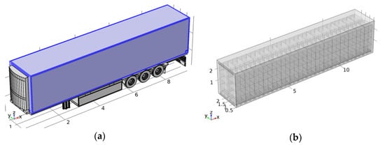
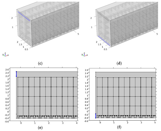
Figure 1.
(a) A general view of the refrigerated semitrailer, (b) fully loaded with the palletized cargo, (c) the location of the inlet, (d) the location of the outlet, (e) the highlighted inlet (on the upper left corner) of the cross-section (2D) of the palletized cargo, (f) the highlighted outlet (on the bottom left corner) of the cross-section (2D) of the palletized cargo.
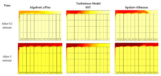
Figure 2.
Transient analysis of the cross-section of the refrigerated trailer model in 2D (single inlet and single outlet on one side).
Although the transient analysis of the refrigerated trailer model is in 2D, which causes a significant divergence of results in comparison with real-world cases, the ventilation of the gaps between the palletized cargoes takes a considerable amount of time (Figure 2). In this model, the inlet and outlet are placed on one side of the trailer.
The RSM is used to illustrate the airflow inside the trailer body (Figure 3). Figure 3a shows the velocity magnitude, Figure 3b shows the external temperature of the trailer body, and Figure 3c depicts the internal temperature distribution. Airflow velocity and temperature drops are observed on the upper-back side of the trailer body.
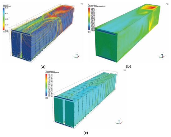
Figure 3.
The stationary model of turbulent flow, method: Reynolds stress model (RSM) (a) streamline: velocity magnitude (m/s), (b) external temperature (°C) distribution, (c) internal temperature (°C) distribution.
In this model, cold air is blown from the inlet at the top of the trailer (front) and the air returns to the outlet at the bottom. Starting from the inlet, the cold air stream makes turns to avoid the obstacles, which are palletized cargo, and moves toward the empty zones, and the air stream sweeps through the trailer body until reaching the outlet. Low air velocity (Figure 3a) and high product temperature (Figure 3b,c) are observed at the rear. By contrast, high air velocity and low air temperature at the front might lead to partial product chilling. Further, a higher blowing air velocity might result in a lower maximum and mean temperature distribution, as having a higher blowing air velocity from the inlet might improve the temperature distribution inside the trailer body. However, in practice, the blowing air velocity is limited by the equipment manufacturers’ specifications.
4.2. Model 2: Three Elongated Inlets on the Ceiling and a Single Outlet on One Side
In this model, three elongated inlets are placed on the ceiling of the trailer. The outlet is placed on one side.
In Figure 4, the locations of the inlets and outlet of the reduced-scale refrigerated trailer are illustrated. Figure 4a illustrates the inlets highlighted on the ceiling of the trailer body, Figure 4b illustrates a close-up view of the inlets, which are highlighted, and Figure 4c illustrates the location of the outlet.
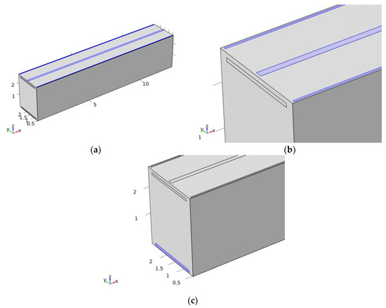
Figure 4.
Location of inlets and outlet (a) inlets are highlighted on the ceiling of the container, (b) close-up view of the inlets (highlighted), (c) outlet (highlighted).
The RSM is used to investigate the airflow inside the trailer body (Figure 5). Figure 5a shows the velocity magnitude, Figure 5b shows the external temperature of the trailer body, and Figure 5c depicts the internal temperature distribution. Temperature increases are observed at the back of the trailer body (Figure 5b).
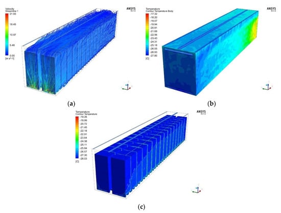
Figure 5.
The stationary model of turbulent flow, method: RSM (a) streamline: velocity magnitude (m/s), (b) external temperature (°C) distribution, (c) internal temperature (°C) distribution.
In this model, starting from the elongated inlets on the ceiling of the trailer body, the cold air stream makes turns to avoid the palletized cargo and moves toward the empty zones, and the air stream sweeps through the trailer body until reaching the outlet. The model presents the contour plot of temperature distribution for the simulation. Wherever the air velocity is high, such as in the main airflow or in the circulations close to the outlets, the temperature is lower due to the low temperature air supplied from the inlets.
4.3. Model 3: Three Elongated Inlets on the Ceiling and Two Outlets on Two Sides
In this model, three elongated inlets are placed on the ceiling of the trailer. The outlets are placed on two sides.
Figure 6 illustrates the locations of the inlets and outlet. Figure 6a illustrates the inlets highlighted on the ceiling of the trailer body, Figure 6b illustrates a close-up view of the inlets, which are highlighted, and Figure 6c,d illustrates the locations of the outlets.
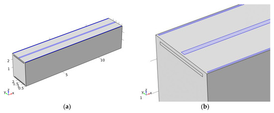
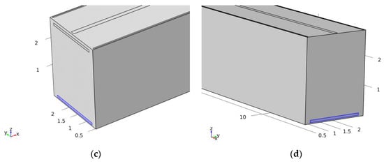
Figure 6.
Location of inlets and outlets; (a) inlets are highlighted on the ceiling of the container, (b) close-up view of the inlets (highlighted), (c) outlet 1 (highlighted), (d) outlet 2 (highlighted).
The RSM is used to depict the airflow inside the trailer body (Figure 7). Figure 7a shows the velocity magnitude, Figure 7b shows the external temperature of the trailer body, and Figure 7c depicts the internal temperature distribution.
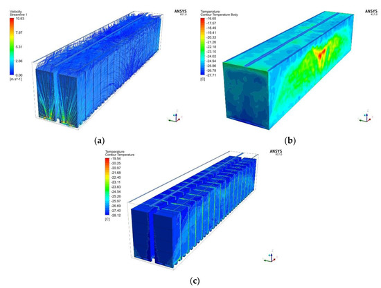
Figure 7.
The stationary model of turbulent flow, method: RSM (a) streamline: velocity magnitude (m/s), (b) external temperature (°C) distribution, (c) internal temperature (°C) distribution.
In this model, starting from the elongated inlets on the ceiling of the trailer body, the cold air stream makes turns to avoid the palletized cargo and moves toward the empty zones, and the air stream sweeps through the trailer body until reaching the outlets. The second outlet is placed at the back of the trailer to overcome the backward heating problem of the previous model. However, this time, temperature increases are observed in the middle of the trailer body (Figure 7b).
In Figure 8, the bold spikes indicate the significant temperature and kinetic energy changes between the gaps of palletized cargo inside the refrigerated vehicle. Although the forced air circulation does not create the significant movement of cold air in the gaps of the palletized cargo, it maintains higher temperature levels. There is heat transfer from the walls of the trailer body; however, the circulation of cold air is strong enough to sweep that wall and this effectively removes the heat from it. In Model 2, high temperature regions are found at the back of the trailer body, whereas in Model 3, high temperature regions are found in the middle, as the heat flux from outside comes through there without any significantly strong cold airflow to remove it.
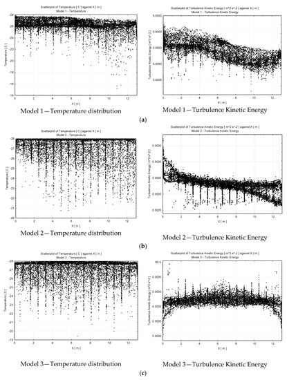
Figure 8.
Temperature and turbulence kinetic energy distributions along the x axis of the trailer with sample sizes of 10,000. (a) Model 1: Single outlet–single inlet, (b) Model 2: Single outlet–multiple inlets, (c) Model 3: Multiple outlets–multiple inlets.
4.4. Statistical Analysis of the Temperature Data
To assess the cooling efficiency of the three models, Levene’s test is performed to check for the existence of statistical significance (Table 2).
Table 2.
Levene’s test.
The statistics in Table 3 test the null hypothesis that the standard deviations in each of the three columns are the same. Of particular interest is the p-value. Since these values are all less than 0.05, there is a statistically significant difference among the standard deviations at the 95% confidence level. This violates one of the important assumptions underlying the analysis of variance and will invalidate most standard statistical tests. Table 3 also compares the standard deviations for each pair of samples. The two p-values below 0.05 indicate a statistically significant difference between the two sigmas at the 5% significance level.
Table 3.
Variance check.
Table 4 shows the summary statistics for the selected variables of the models. The table includes measures of central tendency, measures of variability and measures of the shape of the distribution. In this case, standardized skewness and standardized kurtosis are particularly interesting. They are used to determine if the sample comes from a normal distribution. Standardized skewness and standardized kurtosis values outside the range of −2 to +2 indicate significant deviations from normality, which would invalidate many of the statistical procedures normally applied to these data. In this case, all variables show standardized skewness values outside the expected range. Therefore, Mood’s median test is performed to test the hypothesis that the medians of the three samples are equal (Table 5).
Table 4.
Summary statistics of the temperature variables of the three models.
Table 5.
Mood’s median test, total n = 5826, grand median = −26.987.
Mood’s median test counts the number of observations in each sample on either side of the grand median. Since the p-value equals 0 for the chi-square test (test statistic = 2424.75) and it is less than 0.05, the medians of the samples are significantly different at the 95% confidence level. Also included are the 95% confidence intervals for each median based on the order statistics of each sample (Model 1, 2, and 3).
Figure 9a depicts the box-and-whisker plots of the temperature distributions of Models 1, 2, and 3 and Figure 9b shows the quantile plots of the temperature proportions of Models 1, 2, and 3. Figure 9a illustrates the essential features of the temperature data of the models. The box-and-whisker plot summarizes the temperature data samples by using five statistics, namely minimum, lower quartile, median, upper quartile, and maximum. It also indicates the presence of outliers. In Figure 9b, the quantile plot displays the empirical cumulative distributions of the temperature data. The data are sorted from smallest to largest and plotted at the coordinates.
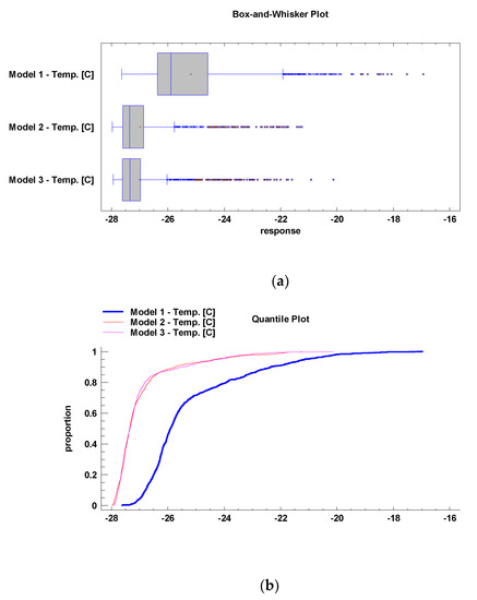
Figure 9.
(a) Box-and-whisker plots of the temperature distributions of Models 1, 2, and 3, (b) quantile plots of the temperature proportions of Models 1, 2, and 3.
4.5. Mann–Whitney (Wilcoxon) W-Test to Compare the Medians of the Temperature Distributions
In this subsection, the Mann–Whitney W-test is used to compare the medians of the two samples of the models. This test is constructed by combining the two samples, sorting the data from smallest to largest, and comparing the average ranks of the two samples in the combined data.
As shown in Table 6, firstly, the comparison of the medians of Model 1 and Model 2 indicates that the p-value is less than 0.05. Therefore, the median of the first sample of Model 1 is significantly greater than the median of the second sample of Model 2 at the 95% confidence level. Secondly, the comparison of the medians of Model 1 and Model 3 reveals that the p-value is less than 0.05. Therefore, as before, the median of the first sample of Model 1 is significantly greater than the median of the second sample of Model 3 at the 95% confidence level. Finally, the comparison of the medians of Model 2 and Model 3 shows that since the p-value is greater than 0.05, there is no statistically significant difference between them at the 95% confidence level.
Table 6.
Mann–Whitney (Wilcoxon) W-test to compare the medians of the models.
5. Conclusions
The simulations effectively showed the airflow and temperature profiles inside the trailer bodies as well as the high and low airflow velocities and cooling regions. The airflow and temperature circulation inside the trailer were demonstrated and quantified by utilizing stream and contour plots. Although Model 1 is the most commonly used refrigerated trailer model in the cold supply chain system, it has significant disadvantages. The analyses of these three models revealed that significant improvement could be achieved by placing multiple elongated inlets on the ceiling of the trailer body. Therefore, Models 2 and 3 appear to have significant advantages over Model 1. In comparison with Model 2, which has only one outlet on one side in the front part, the placement of the additional second outlet in Model 3 aimed to cope with the temperature increase at the back of the trailer. However, with the additional second outlet at the back of the trailer in Model 3, the temperature increases were observed in the middle of the trailer.
Refrigerated vehicles are an essential piece of equipment in the cold supply chain network. Regular refrigerated cargo systems, however, are not designed to support the homogeneity of the temperature inside the cargo, as in Model 1. Typically, refrigerating equipment is placed on one side of the trailer as this is considered to be handier. Under such designs, temperature differences occur in the two far-off parts of the refrigerated payload, which may impact the quality, safety, and shelf life of perishable foods. This study investigated three airflow models of refrigerated cargo systems by applying turbulence flow, heat, and mass transfer models. The analyses revealed that significant improvement could be achieved by applying the proper arrangements of inlets on the ceiling of the trailer body, as shown in Models 2 and 3.
The current research has limitations as it only investigated specific inlet locations and looked only into some of the specific 3D models having elongated inlets on top of the refrigerated trailer models. Therefore, improvements on the body of the trailer are limited. Further research should nevertheless aim to investigate the shape and topology optimization of inlets, outlets, and 3D models of refrigerated trailers. Results from the multi-objective optimization could indicate the location, shape, and size of inlets/outlets, including the optimal topology of the trailer. Such research would shed light on providing a uniform distribution of temperature and heat exchanges inside refrigerated trailers based on intensive calculations involving the principles of mass, momentum, and energy equations. It would also improve many aspects of refrigerated trailers including the consumption of energy.
Funding
This research received no external funding.
Conflicts of Interest
The author declares no conflict of interest.
Nomenclature
| Specific heat at constant pressure | |
| Specific heat at constant volume | |
| Internal energy | |
| Total energy | |
| Enthalpy | |
| Turbulent kinetic energy | |
| Static pressure | |
| Specific gas constant | |
| Traceless viscous strain-rate tensor | |
| Time | |
| Static temperature (Kelvin) | |
| Friction velocity | |
| Velocity | |
| Specific heat ratio = | |
| Turbulence dissipation | |
| Kronecker’s delta function | |
| Dynamic viscosity | |
| Kinematic viscosity | |
| Density | |
| Shear stress tensor | |
| Specific dissipation | |
| Mass fraction of species k | |
| Molar fraction of species k | |
| Molar concentration of species k | |
| Molecular weight of species k | |
| Mean molecular weight of a mixture | |
| k-species reaction rate | |
| Superscript | |
| ′ | Reynolds fluctuating part |
| ″ | Favre fluctuating part |
| Favre Density weighted average | |
| Normal average (time/space) | |
Appendix A
Appendix A.1. The Governing Equations
Appendix A.1.1. Heat Transfer in Fluids (Convection)
Based on the Newton’s Law of Cooling, heat transfer owing to convection is depicted as where is the heat convected to the surrounding fluid (), is the convection coefficient of heat-transfer (constant of proportionality) (), is the area of the solid which is in contact with the fluid (), and is the temperature difference of the solid and the fluid which surrounds it () (). Additionally, the heat transfer (convective) can be characterized in terms of the Nusselt number.
It can be defined as where is the Nusselt number, is the convection coefficient of heat-transfer (constant of proportionality) (), is the characteristic dimension of a solid object (), and is the thermal conductivity of a solid (). The Nusselt number can be considered as the ratio of the convective heat flux to the conduction for a fluid layer. If is equal to 1, it implies that we have a pure conduction. Higher Nusselt values mean that heat transfer is enhanced by convection. Generally, it is written as . In here, “” is the Reynolds number, “” is the Prandtl number, and “” is the Grashof number. It should be noted that the following conditions apply. which is the mixed convection, which is the forced convection, and which is the natural convection.
Appendix A.1.2. Turbulent Flow Algebraic yPlus
Algebraic turbulence models, which are also called zero equation turbulence models are models that do not require the resolution of any additional equations. They are calculated from the flow variables. Such models are generally written as , and they are often used in specific situations, for instance boundary layers or jets.
Appendix A.1.3. Turbulent Flow SST
The kinematic eddy viscosity is , the turbulence kinetic energy is , the specific dissipation rate is , and the closure coefficients and auxiliary relations is , , , and , , , , ,
Appendix A.1.4. Turbulent Flow Spalart–Allmaras
In the turbulent eddy viscosity models, it is given by
where , , , , and
Here the distance to the closest surface is denoted by the d. Constants are , , , , , , , , , , ,
There also exists some modifications of the original model. Spalart indicated that it is safer to use and for the last two constants. Dacles-Mariani et al. [40], on the other hand, suggested some more changes of the model which take into account the effect of average strain rate on the production of turbulence. This changes are depicted as where , , , ,
For the compressible flow models, there are two approaches to adapt the model to compressible flows. For the first approach, the turbulent dynamic viscosity is calculated from
where denotes the local density. The convective terms in the equation for are modified to . Here, the right side (RHS) is identical to that of the original model. By defining values of , the boundary conditions are set. For walls, is equal to 0 and the outlet is a convective outlet.
Appendix A.1.5. Turbulent Flow Reynolds Stress Model (RSM)
The Reynolds stress model involves computation of each of the Reynolds stresses, , using the equations of differential transport. Each of the Reynolds stresses are then utilized to get the closure of the Reynolds-averaged momentum equation. The Reynolds stresses, , of the exact transport equations for the transport can be written as follows.
In a more compact form, it is Local Time Derivate + where is the convection-term, indicates the turbulent diffusion, is the molecular diffusion, stands for stress production, indicates the pressure strain, is for the dissipation and indicates the production by system rotation. Namely the terms, , , , and do not require modeling. On the other hand, , , and must be modeled for closing the equations. To model the pressure–strain term, for the return-to-isotropy models, which is for an anisotropic turbulence, the Reynolds stress tensor, , is generally anisotropic. The second and third invariances of the Reynolds-stress anisotropic tensor are nontrivial, and where and . For modeling turbulent diffusive transport, and modeling the dissipation, the following model constants are suggested .
References
- Oro, E.; Miro, L.; Farid, M.M.; Martin, V.; Cabeza, L.F. Energy management and CO2 mitigation using phase change materials (PCM) for thermal energy storage (TES) in cold storage and transport. Int. J. Refrig. 2014, 42, 26–35. [Google Scholar] [CrossRef]
- Badia-Melis, R.; Garcia-Hierro, J.; Ruiz-Garcia, L.; Jimenez-Ariza, T.; Villalba, J.I.R.; Barreiro, P. Assessing the dynamic behavior of WSN motes and RFID semi-passive tags for temperature monitoring. Comput. Electron. Agric. 2014, 103, 11–16. [Google Scholar] [CrossRef]
- Moureh, J.; Tapsoba, S.; Derens, E.; Flick, D. Air velocity characteristics within vented pallets loaded in a refrigerated vehicle with and without air ducts. Comput. Electron. Agric. 2009, 32, 220–234. [Google Scholar] [CrossRef]
- Moureh, J.; Flick, D. Airflow pattern and temperature distribution in a typical refrigerated truck configuration loaded with pallets. Int. J. Refrig. 2004, 27, 464–474. [Google Scholar] [CrossRef]
- Laguerre, O.; Hoang, H.M.; Flick, D. Experimental investigation and modelling in the food cold chain: Thermal and quality evolution. Trends Food Sci. Technol. 2013, 29, 87–97. [Google Scholar] [CrossRef]
- Tanner, D.J.; Amos, N.D. Temperature variability during shipment of fresh produce. Acta Hortic. 2003, 599, 193–203. [Google Scholar] [CrossRef]
- Moureh, J.; Menia, N.; Flick, D. Numerical and experimental study of airflow in a typical refrigerated truck configuration loaded with pallets. Comput. Electron. Agric. 2002, 34, 25–42. [Google Scholar] [CrossRef]
- Moureh, J.; Tapsoba, M.; Flick, D. Airflow in a slot-ventilated enclosure partially filled with porous boxes: Part II—Measurements and simulations within porous boxes. Comput. Fluids 2009, 38, 206–220. [Google Scholar] [CrossRef]
- Moureh, J.; Tapsoba, M.; Flick, D. Airflow in a slot-ventilated enclosure partially filled with porous boxes: Part I—Measurements and simulations in the clear region. Comput. Fluids 2009, 38, 194–205. [Google Scholar] [CrossRef]
- Rodriguez-Bermejo, J.; Barreiro, P.; Robla, J.I.; Ruiz-Garcia, L. Thermal study of a transport container. J. Food Eng. 2007, 80, 517–527. [Google Scholar] [CrossRef]
- Smale, N.J. Mathematical Modelling of Airflow in Shipping Systems: Model Development and Testing. Ph.D. Thesis, Massey University, Palmerston North, New Zealand, 2004. [Google Scholar]
- Tapsoba, M.; Moureh, J.; Flick, D. Airflow patterns in an enclosure loaded with slotted pallets. Int. J. Refrig. 2006, 29, 899–910. [Google Scholar] [CrossRef]
- Tapsoba, M.; Moureh, J.; Flick, D. Airflow patterns in a slot-ventilated enclosure partially loaded with empty slotted boxes. Int. J. Heat Fluid Flow 2007, 28, 963–977. [Google Scholar] [CrossRef]
- Tapsoba, M.; Moureh, J.; Flick, D. Airflow patterns inside slotted obstacles in a ventilated enclosure. Comput. Fluids 2007, 36, 935–948. [Google Scholar] [CrossRef]
- Alvarez, G.; Bournet, P.E.; Flick, D. Two-dimensional simulation of turbulent flow and transfer through stacked spheres. Int. J. Heat Mass Transf. 2003, 46, 2459–2469. [Google Scholar] [CrossRef]
- Defraeye, T.; Verboven, P.; Nicolai, B. CFD modelling of flow and scalar exchange of spherical food products: Turbulence and boundary-layer modelling. J. Food Eng. 2013, 114, 495–504. [Google Scholar] [CrossRef]
- Defraeye, T.; Cronje, P.; Berry, T.; Opara, U.L.; East, A.; Hertog, M.; Verboven, P.; Nicolai, B. Towards integrated performance evaluation of future packaging for fresh produce in the cold chain. Trends Food Sci. Technol. 2015, 44, 201–225. [Google Scholar] [CrossRef]
- Defraeye, T.; Cronje, P.; Verboven, P.; Opara, U.L.; Nicolai, B. Exploring ambient loading of citrus fruit into reefer containers for cooling during marine transport using computational fluid dynamics. Postharvest Biol. Technol. 2015, 108, 91–101. [Google Scholar] [CrossRef]
- Defraeye, T.; Verboven, P.; Opara, U.L.; Nicolai, B.; Cronje, P. Feasibility of ambient loading of citrus fruit into refrigerated containers for cooling during marine transport. Biosyst. Eng. 2015, 134, 20–30. [Google Scholar] [CrossRef]
- Moureha, J.; Letang, G.; Palvadeau, B.; Boisson, H. Numerical and experimental investigations on the use of mist flow process in refrigerated display cabinets. Int. J. Refrig. 2009, 32, 203–219. [Google Scholar] [CrossRef]
- Cardinale, T.; Fazio, P.; Grandizio, F. Numerical and experimental computation of airflow in a transport container. Int. J. Heat Technol. 2016, 34, 734–742. [Google Scholar] [CrossRef]
- Cardinale, T.; De Fazio, P.; Grandizio, F. Numerical and experimental computation of airflow in a transport container. Int. J. Heat Technol. 2016, 34, S323–S331. [Google Scholar] [CrossRef]
- Katai, L.; Varszegi, T.; Oldal, I.; Zsidai, L. Hydrodynamic modelling and analysis of a new-developed mobile refrigerated container. Acta Polytech. Hung. 2016, 13, 83–104. [Google Scholar] [CrossRef]
- Getahun, S.; Ambaw, A.; Delele, M.; Meyer, C.J.; Opara, U.L. Analysis of airflow and heat transfer inside fruit packed refrigerated shipping container: Part I—Model development and validation. J. Food Eng. 2017, 203, 58–68. [Google Scholar] [CrossRef]
- Getahun, S.; Ambaw, A.; Delele, M.; Meyer, C.J.; Opara, U.L. Analysis of airflow and heat transfer inside fruit packed refrigerated shipping container: Part II—Evaluation of apple packaging design and vertical flow resistance. J. Food Eng. 2017, 203, 83–94. [Google Scholar] [CrossRef]
- Kan, A.K.; Hu, J.; Guo, Z.P.; Meng, C.; Chao, C. Impact of cargo stacking modes on temperature distribution inside marine reefer containers. Int. J. Air Cond. Refrig. 2017, 25. [Google Scholar] [CrossRef]
- Han, J.W.; Zhao, C.J.; Yang, X.T.; Qian, J.P.; Xing, B. Computational fluid dynamics simulation to determine combined mode to conserve energy in refrigerated vehicles. J. Food Process. Eng. 2016, 39, 186–195. [Google Scholar] [CrossRef]
- Smale, N.J.; Moureh, J.; Cortella, G. A review of numerical models of airflow in refrigerated food applications. Int. J. Refrig. 2006, 29, 911–930. [Google Scholar] [CrossRef]
- Puška, A.; Maksimović, A.; Stojanović, I. Improving organizational learning by sharing information through innovative supply chain in agro-food companies from Bosnia and Herzegovina. Oper. Res. Eng. Sci. Theory Appl. 2019, 1, 76–90. [Google Scholar] [CrossRef]
- Fazlollahtabar, H. Operations and inspection cost minimization for a reverse supply chain. Oper. Res. Eng. Sci. Theory Appl. 2019, 1, 91–107. [Google Scholar] [CrossRef]
- Badi, I.; Ballem, M. Supplier selection using rough BWM-MAIRCA model: A case study in pharmaceutical supplying in Libya. Decis. Mak. Appl. Manag. Eng. 2018, 1, 16–33. [Google Scholar] [CrossRef]
- Menter, F. Zonal two equation k-w turbulence models for aerodynamic flows. In 23rd Fluid Dynamics, Plasmadynamics, and Lasers Conference; American Institute of Aeronautics and Astronautics: Reston, VA, USA, 1993. [Google Scholar]
- Menter, F.R. Two-equation eddy-viscosity turbulence models for engineering applications. AIAA J. 1994, 32, 1598–1605. [Google Scholar] [CrossRef]
- Spalart, P.; Allmaras, S. A one-equation turbulence model for aerodynamic flows. In 30th Aerospace Sciences Meeting and Exhibit; American Institute of Aeronautics and Astronautics: Reston, VA, USA, 1992. [Google Scholar]
- Spalart, P.R.; Allmaras, S.R. A one-equation turbulence model for aerodynamic flows. In Proceedings of the 30th AIAA Aerospace Sciences Meeting and Exhibit, Reno, NV, USA, 6–9 January 1992; pp. 5–21. [Google Scholar]
- Chou, P.Y. On velocity correlations and the solutions of the equations of turbulent fluctuation. Q. Appl. Math. 1945, 3, 38–54. [Google Scholar] [CrossRef]
- Rotta, J. Statistische theorie nichthomogener turbulenz. Z. Phys. 1951, 129, 547–572. [Google Scholar] [CrossRef]
- Sun, D.-W. Computational Fluid Dynamics in Food Processing, 2nd ed.; Sun, D.-W., Ed.; CRC Press: Boca Raton, FL, USA, 2018. [Google Scholar]
- Glouannec, P.; Michel, B.; Delamarre, G.; Grohens, Y. Experimental and numerical study of heat transfer across insulation wall of a refrigerated integral panel van. Appl. Therm. Eng. 2014, 73, 196–204. [Google Scholar] [CrossRef]
- Daclesmariani, J.; Zilliac, G.G.; Chow, J.S.; Bradshaw, P. Numerical experimental—Study of a wingtip Vortex in the near-field. AIAA J. 1995, 33, 1561–1568. [Google Scholar] [CrossRef]
© 2019 by the author. Licensee MDPI, Basel, Switzerland. This article is an open access article distributed under the terms and conditions of the Creative Commons Attribution (CC BY) license (http://creativecommons.org/licenses/by/4.0/).