The “Polluter Pays” Principle in Transportation: The Impact of Environmental Taxes on CO₂ Emissions in V4 Countries

Abstract

Background: Transport remains one of the hardest sectors to decarbonize in the European Union, and the effectiveness of environmental taxation as a “polluter pays” instrument remains contested for the institutionally distinct Visegrad Four (V4) countries. Methods: Using a balanced panel of four V4 countries over 2000–2024 (n = 100 observations) from Eurostat, we estimate fixed-effects models with Driscoll–Kraay standard errors, complemented by two-way fixed effects, lag, interaction, and robustness specifications, including a sensitivity test for mechanical endogeneity. Results: GDP per capita and freight transport volume are positively associated with emissions (elasticities 0.244 and 0.230, both p < 0.001), while renewable energy share is negatively associated (−2.93%, p < 0.001). Environmental taxes show no significant association at any lag, and their positive association is strongest where highway infrastructure is least developed, disappearing where it is most developed. Freight transport remains the only robust driver once year effects are controlled for; a tax-to-freight intensity indicator reveals a significant three-year lag effect. Conclusions: Environmental taxation alone is not robustly associated with lower transport emissions in the V4; its association is conditional on infrastructure development and best complemented by renewable-energy investment. Findings should be read as descriptive associations rather than causal effects.

1. Introduction

Transport is one of the most significant challenges facing current climate policy, not only because of its share of total emissions, but especially because of the sector’s persistent resistance to decarbonization. In 2018, transportation produced 8.5 GtCO₂eq, accounting for approximately 14% of all direct and indirect global greenhouse gas emissions, with road transportation (both passenger and freight) contributing as much as 73% of this total. Since 1990, emissions from transportation have grown at a rate of approximately 2% per year, primarily because, in most regions, the growth in mobility and transport volume has outweighed the savings achieved through improvements in energy and fuel efficiency [1]. This pattern differs from developments in other sectors, such as the energy sector, where the transition toward low-carbon sources has progressed more significantly [2].

It is precisely this structural inertia that makes transportation one of the most difficult sectors to decarbonize: even the most economically advanced countries have not yet achieved significant absolute reductions in transportation emissions [1]. The reason is the close link between demand for mobility, trade, economic growth, and energy consumption in transportation; decarbonization therefore cannot rely on a single tool but must simultaneously combine technological change, infrastructure development, and demand management [1,3].

In the European context, transportation is a key component of the climate agenda of the European Green Deal and the “Fit for 55” package, which link the reduction in transportation emissions to a broader transition toward clean mobility, electrification, and the development of renewable energy sources [4]. While the electricity sector in the EU is decarbonizing relatively quickly, transportation is lagging because energy consumption in this sector closely tracks the growth of gross domestic product (GDP) per capita and the rising demand for the transport of both goods and people [1,3]. The Visegrad Four (V4) countries, namely the Czech Republic, Poland, Slovakia, and Hungary, represent a specific case within the EU: their economies are highly export-oriented, their industrial and logistical structures rely heavily on freight transport, and the long-term process of catching up in living standards has historically led to faster growth in demand for mobility than in more developed member states. The question of how economic instruments, such as environmental taxes, can affect transportation emissions in this specific regional context thus takes on particular significance.

1.1. From the “Polluter Pays” Principle to Transport Taxation: A Conceptual Clarification

Before reviewing empirical evidence, it is useful to clarify the conceptual chain that links the “polluter pays” principle to the specific tax variable used in this study, since these terms are often used interchangeably in the applied literature despite referring to distinct policy instruments. The “polluter pays” principle is a normative, allocative rule stating that the economic costs of pollution should be borne by those who cause it rather than by society at large. Its standard economic operationalization is Pigouvian taxation: a per-unit tax on a polluting activity set, in principle, equals to the marginal external damage it causes, so that the private cost of the activity comes to reflect its full social cost. Carbon pricing, whether implemented as an explicit carbon tax or through an emissions-trading scheme such as the EU ETS, is the closest real-world approximation of a Pigouvian instrument, because its base is defined directly in terms of CO₂ (or CO₂-equivalent) emitted. Fuel excise duties and vehicle taxes (registration or ownership taxes, road tolls) are second-best approximations: their tax base is a proxy correlated with emissions (fuel consumed, engine size, vehicle weight or age) rather than emissions themselves, so their environmental incidence depends on how tightly that proxy tracks actual pollution. Finally, statistical aggregates such as Eurostat’s “environmental taxes” series are a broader accounting category that bundles energy, transport, and pollution/resource taxes according to whether their tax base has a proven, specific negative impact on the environment, regardless of the policy intention behind their original introduction (which, for fuel excises in particular, was frequently revenue generation rather than environmental correction).

This study operationalizes the “polluter pays” principle using Eurostat’s “environmental taxes classified by economic activity, transport-related component” series, which is dominated by fuel excise duties and vehicle-related taxes rather than an explicit carbon price. This places our tax variable conceptually closer to the “second-best,” proxy-based end of the spectrum described above than to a Pigouvian carbon tax, a distinction that turns out to matter considerably for interpreting our results and is consistent with recent evidence, reviewed in Section 4.3, that the environmental effectiveness of “environmental taxes” varies systematically with exactly this kind of instrument-type heterogeneity.

1.2. Determinants of Transport Emissions

Environmental taxes in transportation represent a key economic instrument of climate policy based on the “polluter pays” principle. Their rationale lies in the internalization of external costs associated with emissions: taxing carbon-intensive activities is intended to increase their relative price compared to cleaner alternatives, thereby steering both consumer and investment decisions toward low-emission modes of transportation, vehicles, and fuels [5,6].

In theory, environmental taxes in transportation operate through several interconnected mechanisms: they promote a modal shift, that is, a shift in demand from carbon-intensive road transport to alternatives with lower emissions (such as rail transport) reduce overall demand for the most polluting forms of transport and simultaneously create an incentive for investment in green technologies [5]. An empirical example of the effectiveness of this mechanism is the Chinese freight corridor, where a carbon tax of $200/tCO₂ reduced emissions by 14.2% precisely through the shift in freight from road to rail transport [5].

However, the expected benefits of environmental taxes are accompanied by significant limitations. Several studies point out that a carbon tax alone is often insufficient to achieve significant emissions reductions unless it is accompanied by complementary policies [5]. An analysis across OECD countries has shown that poorly designed or inadequately targeted taxes may have only a weak, or even counterproductive, effect if they are not combined with investments in public transportation, incentives for purchasing electric vehicles, and the development of sustainable infrastructure. It is precisely the design of the policy, therefore, that emerges as the decisive factor determining whether the effect of an environmental tax will be significantly reductive or merely marginal [6].

The empirical literature from 2020 to 2025 provides relatively consistent yet nuanced evidence on the determinants of transportation emissions. Regarding environmental taxes themselves, many studies confirm their emission-reducing effect. In a panel of 20 European countries, total taxes, energy taxes, and transport-specific taxes were statistically significantly negatively associated with CO₂ emissions [7]. An analysis of the relationship between the green transportation sector, environmental taxes, and related public expenditures reached a similar conclusion, confirming their mitigating effect on transportation CO₂ emissions [8]. Similarly, in the case of Latvia, existing environmental taxes demonstrably reduced transportation emissions, although the authors also emphasized that the decisive factor remains the reduction in fossil fuel consumption and the promotion of clean mobility—meaning that the tax alone is not a sufficient condition for transformation [9]. This line of research thus agrees that environmental taxes work in the desired direction, but their effectiveness depends on complementary policies; without accompanying investments in infrastructure and alternative modes of transportation, the price signal alone remains insufficient [5,6].

A second line of research focuses on the role of freight transport, which most studies consistently identify as the primary source of emissions growth in the sector [1,10]. Global freight activity has increased by 68% over the past two decades [1], although the mechanisms through which this increase translates into emissions vary across countries and levels of analysis. In Shenzhen, for example, it has been shown that the spatial determinants of emissions from road freight transport are primarily related to land-use patterns and the availability of logistics hubs, thereby linking the issue to urban form and infrastructure planning [11]. At the global level, suboptimal logistics routes can also significantly increase emissions; estimates related to disruptions in trade routes after 2022 suggest an additional 630–690 Mt CO₂-eq per year [12]. Freight transport thus appears to be a factor whose impact on emissions is not only consistently positive but also structurally linked to infrastructure and the logistics organization of the economy.

A third line of research focuses on the relationship between GDP per capita and transportation emissions, where the evidence is less consistent. A positive relationship predominates; in Indonesia, GDP per capita had a positive and significant effect on emissions in both the short and long term [13,14]. However, some studies find nonlinearity consistent with the Environmental Kuznets Curve (EKC): in a global panel of 154 countries, the relationship between GDP per capita and emissions was nonlinear, with the contribution of income growth to emissions gradually weakening as GDP levels rose [15]. In the North American panel, although per capita income was generally positively associated with emissions, only a subset of countries lay beyond the inflection point of the inverted U curve [16]. This discrepancy suggests that the relationship between economic growth and transportation emissions is not universal but depends on the structure of the economy and the stage of development of a given country, which is particularly relevant for the V4 countries, which have historically been in the process of catching up economically.

Finally, the fourth line of analysis concerns renewable energy sources in transportation, where the evidence is most consistent. In the EU, higher adoption of renewable energy was associated with a decline in transportation CO₂ emissions [4]. In China, both renewable energy and technological innovations had a negative (i.e., reduction) impact on transportation emissions, while GDP had the opposite effect [17]. At the same time, however, integrated decarbonization models suggest that renewable energy will remain a relatively scarce resource in the coming decades; therefore, it may be more effective to first decarbonize the power grid and only then proceed to further electrify transportation itself [3]. This perspective partially tempers expectations regarding the rapid expansion of renewable energy directly within the transportation sector and highlights the need for a sequential, rather than concurrent, approach to the decarbonization of the energy and transportation sectors.

The current state of research provides compelling evidence that transportation is a structurally challenging sector, environmental taxes have a predominantly reductive but conditional effect, freight transportation acts as a consistent source of emissions growth, GDP per capita has a predominantly positive effect, though with varying degrees of nonlinearity, and renewable energy reduces emissions, although its actual potential in transportation is time limited. Key discrepancies in the literature therefore do not concern the sector’s significance per se, but rather the strength of the effect of environmental taxes, the form of nonlinearity in the GDP emissions relationship, and the question of whether technological progress and infrastructure alone are sufficient without deeper changes in logistics and the structure of demand [5,6,15,16].

1.3. Institutional and Structural Distinctiveness of the V4 Countries

The V4 countries also lag behind the EU-28 average in circular-economy efficiency, though they have been gradually converging toward it: among the V4, Poland has achieved the highest circular-economy efficiency, while Slovakia has recorded the weakest average results, converging markedly with the rest of the group between 2015 and 2017 [18]. A higher GDP level does not guarantee higher circular-economy efficiency, suggesting that structural and institutional factors, rather than income alone, play a decisive role [18]. This structural legacy is also visible in the transition away from the heavy, energy-intensive industry of the communist period: in Czechia, industry’s share of final energy consumption fell from 48.26% to 24.83% as many state enterprises collapsed and Western European production patterns were implemented only after EU accession in 2004 [19]. A cluster analysis of energy consumption groups Poland, Czechia, and Hungary together with most Western European countries, while Slovakia remains in a distinct cluster characterized by a persistently higher industrial share of energy consumption [19].

The V4 countries’ transport sectors diverge from those of established EU member states in both historical trajectory and current energy-security profile. Road transport expanded rapidly across V4 after the fall of communism, in contrast to the relative stabilization of transport’s share of economic activity observed in established EU member states over the same period [19]. The V4 also began their energy-security transition later than the “old” EU; within the group, Czechia leads on sustainable energy security while Poland ranks lowest [20]. In Czechia specifically, transport’s share of final energy consumption rose from 7.86% to 24.60%, reflecting a shift away from the rail-based transport typical of heavy industry toward road transport [19]; despite this shift, the V4 countries as a whole have not closed the energy-efficiency gap with the EU average, plausibly because modern efficiency technologies were adopted more quickly in Western Europe [19].

Beyond these general mechanisms, the V4 countries differ from the “old” EU-15 member states along several further dimensions that are directly relevant to how environmental transport taxation is likely to function. First, the V4’s tax structures and revenue mixes remain heterogeneous: government expenditure and growth linkages of environmental tax revenue in V4 have been shown to differ from Western European patterns, with a weaker and less consistent association between environmental tax receipts and green public investment [21]. This divergence extends to the broader macro-fiscal regime: Czechia and Poland exhibit stable monetary dominance grounded in strict Ricardian fiscal discipline, Hungary suffers from structural fiscal dominance and serious institutional conflict, and Slovakia shows persistent fiscal dominance that is nonetheless insulated from macroeconomic destabilization by its eurozone membership [22]. Absolute tax revenues also differ substantially across the group Poland reported USD 134.63 billion in tax revenue compared to USD 23.7 billion in Slovakia and EU enlargement itself has been shown to significantly affect V4 tax revenues both in the short and the long run [23]. Public expenditure across the region has also tended to flow more often toward wages and pensions than toward productive investment with multiplier effects, and corruption has been shown to weaken the effect of government fiscal policy on competitiveness, with the V4 facing higher levels of corruption than their western neighbors; despite more than a decade of EU membership, the V4 countries have not substantially closed the competitiveness gap with Western Europe, partly because of this institutional fragility and political instability [24]. Even where EU-wide convergence in environmental taxation is observed—one recent panel study finds a convergent trend specifically in transport-tax revenues across EU countries, in contrast to other categories of environmental taxation—catching-up economies such as the V4 combine lower absolute tax rates with a revenue structure more dependent on fuel excises than on carbon pricing [25]. Second, the V4 industrial base is more logistics- and export-intensive relative to GDP than the EU-15 average, with a correspondingly higher share of freight moved by road rather than rail or inland waterway, reflecting both historically limited investment in rail-freight infrastructure and the more recent integration of V4 manufacturing (notably automotive and electronics) into pan-European just-in-time supply chains. Taken together, these institutional and structural differences imply that price signals calibrated to, or estimated from, Western European data need not transfer directly to the V4 context, reinforcing the case for a region-specific empirical assessment.

1.4. Logistics and Freight-Transport Relevance

Because the V4 economies are strongly export-oriented and embedded in cross-border European supply chains, the question addressed in this study is, at its core, a logistics question as much as an environmental-economics one. Freight transport in the V4 is organized predominantly around a small number of road corridors connecting manufacturing clusters (notably automotive and electronics production in Slovakia, Czechia, and Hungary) to Western European and, increasingly, intra-regional markets, largely along TEN-T core network corridors (e.g., the Baltic–Adriatic and Orient/East-Med corridors) that pass through the region. This corridor structure means that decisions nominally about “transport taxation” are, in practice, decisions about the routing, mode choice, and cost structure of logistics operators and freight forwarders who plan shipments across national borders rather than within a single domestic market. Section 4.6 returns to this logistics-operator perspective when interpreting our results, in particular the finding that infrastructure development moderates the tax–emissions relationship.

Despite the relatively extensive empirical literature on the relationship between environmental taxes, freight transport, GDP per capita, renewable energy sources, and transportation emissions, existing studies focus primarily on large economies (China, the U.S.), homogeneous panels of Western European countries, or individual national cases outside Central Europe (such as Latvia or Indonesia) [7,9,13,14,17]. The V4 countries represent a distinct group with a strongly export-oriented industrial structure, high dependence on road freight transport, and different dynamics of income convergence and environmental-tax structure compared to the “old” EU member states, on which most of the existing European evidence is based [4,7,21,23,25]. At the same time, the question remains open as to how, in this specific regional context, the combined effect of environmental taxes, freight transport, per capita GDP, renewable energy sources, and transportation infrastructure on greenhouse gas emissions manifests—that is, determinants that the existing literature has examined primarily in isolation or under different geographical and institutional conditions [1,5,6,15]. There is thus a lack of systematic panel analysis that would assess these factors collectively, specifically for the V4 countries in the context of the commitments of the European Green Deal and the “Fit for 55” package.

This study addresses this identified research gap by focusing on testing the “polluter pays” principle in the context of the Visegrad Four countries. The aim of the research is to analyze the association between environmental taxes and CO₂ emissions from transportation in the Czech Republic, Poland, Slovakia, and Hungary, while taking into account other key determinants identified in the existing literature, such as freight transportation, GDP per capita, the share of renewable energy sources, and the development of transportation infrastructure [1,7,9,15,17]. The contribution of this study lies in its joint analysis of these determinants for the V4 region, and, in particular, in documenting the interaction between transport infrastructure and environmental taxation, a region that has thus far been on the periphery of existing empirical literature; to our knowledge, this is among the first studies to test these relationships jointly in this specific regional context. The study thus provides insights relevant not only to academic discussion but also to the formulation of environmental tax policy in the context of fulfilling the EU’s climate commitments.

1.5. Research Question and Hypotheses

Building on the gap identified above, the central research question of this study is: to what extent does the “polluter pays” principle, as implemented through environmental taxes on transportation, contribute to reducing transport-related greenhouse gas emissions in the Visegrad Four countries, once economic development, freight transport activity, transport infrastructure, and renewable energy use are taken into account, and how sensitive is this contribution to the way environmental taxation is measured, to the time horizon considered, and to the level of infrastructure development? This question is decomposed into five testable propositions, which structure the empirical analysis in Section 3 and are revisited explicitly in the Conclusions (Section 5):

H1. 

Freight transport volume and GDP per capita are positively associated with transport GHG emissions in the V4 countries.

H2. 

The share of renewable energy in transportation is negatively associated with transport GHG emissions, and this association may persist over more than one year.

H3. 

Environmental taxes on transportation (as a share of GDP) are negatively associated with transport GHG emissions, either contemporaneously or with a one- to three-year lag.

H4. 

The strength of the association between environmental taxes and emissions depends on the level of transport-infrastructure development (i.e., infrastructure moderates the tax–emissions relationship).

H5. 

The estimated association between environmental taxation and transport emissions is sensitive to how environmental tax intensity is operationalized.

2. Materials and Methods

All data used in this study was obtained from Eurostat, the statistical office of the European Union, the missing values were supplemented using data from national statistical offices. Eurostat provides harmonized, publicly available annual panel data across EU member states, which ensures cross-country comparability for the Visegrad Four (V4) countries analyzed in this study. The analysis is based on a balanced panel of N = 4 countries (the Czech Republic, Hungary, Poland, and Slovakia) observed over T = 25 years (2000–2024), yielding a total of n = 100 country-year observations. All statistical and econometric analyses, calculations, and graphical outputs were performed using MATLAB R2026a (MathWorks, Natick, MA, USA).

The dependent variable is greenhouse gas emissions from transportation (in thousand metric tons), obtained from Eurostat’s greenhouse gas emissions inventory data disaggregated by source sector, using the transport sector aggregate covering road (passenger and freight), rail, inland navigation, and other transport modes. The following explanatory variables, all obtained from Eurostat, were included in the analysis:

• GDP per capita (EUR), obtained from Eurostat’s national accounts statistics, used as a proxy for the overall level of economic development and transport demand in each country and year.
• Length of highways and e-roads (km), obtained from Eurostat’s transport infrastructure statistics, used as a proxy for the extent of the road transport network.
• Freight transport volume, measured in million tonne-kilometers (tkm), obtained from Eurostat’s freight transport statistics, capturing the intensity of goods transport activity.
• Environmental taxes on transportation as a share of GDP, obtained from Eurostat’s environmental tax revenue statistics (environmental taxes classified by economic activity, transport-related component), used to operationalize the “polluter pays” principle.
• Renewable energy in transportation (%), obtained from Eurostat’s renewable energy statistics, reflecting the share of renewable energy sources in the final energy consumption of the transport sector.
• For the robustness check, an additional indicator, the “tax-to-freight intensity” (TFI), was constructed by dividing absolute environmental tax revenue on transportation (recovered from Eurostat’s GDP-share series using GDP per capita and total population, the latter obtained from World Bank population statistics) by freight transport volume (rather than by GDP or by emissions), so as to capture the tax burden per unit of freight activity the transport-sector variable most directly implicated in generating emissions, without dividing by the dependent variable itself.

Given the pronounced right-skewed distribution of several variables, greenhouse gas emissions from transportation, GDP per capita, freight transport volume, the share of environmental taxes on transportation in GDP, and the tax-to-freight indicator were transformed using the natural logarithm prior to estimation. The length of highways and e-roads and the share of renewable energy in transportation were retained in their original units owing to their low skewness. Beyond correcting distributional asymmetry, the logarithmic transformation allows the corresponding regression coefficients to be interpreted directly as elasticities.

Descriptive statistics (mean, median, standard deviation, minimum, maximum, and skewness) were computed for all variables in their original units to assess their distributional characteristics and to justify the transformation strategy. A Pearson correlation matrix was then constructed to assess the strength and direction of the bivariate relationships among the variables and to obtain a preliminary indication of multicollinearity risk. This was subsequently verified formally by calculating Variance Inflation Factors (VIFs) for all explanatory variables included in the regression models. A panel regression model of the following form was used to examine the determinants of greenhouse gas emissions

$$ln\left(GH{G}_{it}\right)={\beta }_0+{\beta }_{1}ln\left(GDPP{C}_{it}\right)+{\beta }_{2}ln\left(MOTORWAY{S}_{it}\right)+{\beta }_{3}ln\left(FREIGH{T}_{it}\right)+{\beta }_{4}TA{X}_{it}+{\beta }_{5}ln\left(RENE{W}_{it}\right)+{\mu }_i+{\epsilon }_{it}$$

(1)

where the dependent variable of the model is greenhouse gas emissions from transportation ($GH{G}_{it}$), which represent the volume of emissions produced by the transportation sector in the country during period t. The explanatory variables include gross domestic product per capita ($GDPP{C}_{it}$), which represents the country’s level of economic development; the length of highways and roads in the European E network ($MOTORWAY{S}_{it}$), reflecting the level of road infrastructure development; the volume of freight transport ($FREIGH{T}_{it}$), which captures the intensity of transport activity; the share of environmental taxes on transport in GDP ($TA{X}_{it}$), representing the intensity of environmental taxation in the transport sector; and the share of renewable energy in transport ($RENE{W}_{it}$), which reflects the extent to which renewable energy sources are used in the transport sector. The model also includes an unobserved country-specific effect (${\mu }_i$), which captures the time-invariant characteristics of individual countries, such as geographic location, the historical development of transportation infrastructure, or the structure of the economy, and a random component (${\epsilon }_{it}$), representing the influence of other unobserved factors affecting greenhouse gas emissions. The parameter ${\beta }_0$ represents the model constant (intercept), which expresses the expected value of the dependent variable when all explanatory variables are zero. Parameters ${\beta }_1$ through ${\beta }_n$ represent the regression coefficients of the individual explanatory variables and express the change in the expected value of greenhouse gas emissions for a unit change in the respective variable, if the values of the other variables remain unchanged (ceteris paribus). Since the dependent variable and the selected explanatory variables were transformed using the natural logarithm, the corresponding coefficients can be interpreted as elasticities; that is, they indicate the percentage change in greenhouse gas emissions caused by a 1% change in each explanatory variable.

2.1. Model Selection, Two-Way Fixed Effects, and Treatment of Common Time Shocks

The choice among the three baseline specifications (pooled OLS, fixed effects [FE], and random effects [RE]) was guided first by an F-test for poolability, which tests the joint significance of the country-specific effects against the pooled OLS model. Given the very small number of cross-sectional units (N = 4), the conventional Hausman test comparing the FE and RE estimators was not considered reliably interpretable, since the covariance matrix of the difference between the two estimators becomes numerically close to singular in “narrow but deep” panels with small N; the choice of the fixed-effects specification was therefore additionally supported by substantive arguments regarding the likely correlation between the country-specific effects and the explanatory variables [26].

A one-way (country) fixed-effects model absorbs time-invariant heterogeneity across countries but does not, by itself, control for factors that vary over time but are common to all four countries such as the 2008–2009 global financial crisis, the EU-wide COVID-19 mobility restrictions of 2020, or Europe-wide energy-price shocks following 2021/2022. If such common shocks are correlated with both the regressors (e.g., GDP per capita, which fell across all four countries in 2009 and 2020) and the residual, the one-way FE estimates could partly reflect shared trends rather than genuine within-country responses. To address this concern directly, we therefore re-estimated the baseline model with a full set of year dummies added to the country fixed effects (a “two-way” fixed-effects specification) and tested the joint significance of the year effects with an F-test comparing the restricted (country-only) and unrestricted (country + year) residual sums of squares. We report and discuss the two-way FE results as a dedicated robustness check in Section 3.3, alongside the one-way FE results that remain our baseline specification for the lag, interaction, and robustness analyses that follow.

Conventional panel unit-root tests (e.g., Levin–Lin–Chu, Im–Pesaran–Shin, or Fisher-type tests) have limited inferential power with only N = 4 cross-sectional units, so a non-rejection (or rejection) of the null hypothesis in this setting would not be informative, and such tests are therefore not relied upon as decisive diagnostics in this study. Instead, year fixed effects are introduced to absorb common, economy-wide time shocks and shared regional trends across the four countries (e.g., the 2008–2009 financial crisis, the 2020 COVID-19 mobility restrictions, post-2021 energy-price movements). This addresses a related but distinct concern, spurious correlation driven by trends common to all units—rather than substituting for a formal stationarity test. The persistence of the underlying series (e.g., an average within-country autocorrelation of log-emissions at a three-year lag of 0.62) is explicitly acknowledged as a limitation to bear in mind when interpreting lag structures.

2.2. Diagnostic Testing, Lag Structure, Interaction, and Robustness Specifications

Once the fixed-effects specification was selected, the standard assumptions of panel regression were tested prior to interpretation of the coefficients: the Breusch–Pagan test for homoscedasticity, the Wooldridge test for first-order autocorrelation, and Pesaran’s CD test for cross-sectional dependence. Given the evidence of heteroscedasticity and autocorrelation, all final models were estimated using Driscoll–Kraay robust standard errors, with a Bartlett kernel and a lag truncation selected according to the Newey–West rule, which remain consistent under heteroscedasticity, autocorrelation, and cross-sectional dependence of the residuals. Nevertheless, because the cross-sectional dimension is very small (N = 4), finite-sample inference based on Driscoll–Kraay standard errors should be interpreted cautiously. We therefore use DK standard errors as a robustness-oriented correction rather than as a substitute for the limitations imposed by the narrow cross-sectional dimension of the panel.

To examine whether the association of environmental taxation on transportation emissions manifests with a delay, the baseline fixed-effects model was extended to include one-, two-, and three-year lags of the logarithm of the environmental tax variable. These lags were estimated separately from lags of the renewable energy variable, to preserve degrees of freedom given the limited number of cross-sectional units (N = 4). To test whether the association of environmental taxation depends on the level of development of transport infrastructure, an interaction term between the logarithm of environmental taxes and the length of the highway and e-road network was additionally included in a separate specification, and the marginal effects of environmental taxation on emissions were computed at low (mean − 1 SD), average, and high (mean + 1 SD) levels of highway network length.

As a robustness check, the baseline model was re-estimated by replacing the variable “environmental taxes on transportation as a share of GDP” with the tax-to-freight intensity indicator described above, so as to assess the sensitivity of the results to the choice of denominator used to operationalize the “polluter pays” principle. An earlier version of this robustness check used an emissions-denominated indicator (environmental tax revenue per unit of greenhouse gas emissions); because emissions are also the dependent variable of the model, that construction raised a specific mechanical-endogeneity concern, since any regressor built by dividing by GHG_it (or a lag of it) is, by construction, correlated with GHG_it through the strong own-persistence of emissions over time, independently of any genuine causal channel. The tax-to-freight intensity indicator used here avoids this problem because freight transport volume is an explicitly included control variable in every specification, not the dependent variable.

2.3. Endogeneity and the Feasibility of Instrumental-Variable Identification

A central limitation of the observational panel design used here is the potential for reverse causality between transport activity, tax revenue, and emissions: countries or years with more freight and passenger transport activity mechanically generate both more emissions and more fuel/transport tax revenue (because most environmental tax revenue in the V4 is raised through volume-linked fuel excises rather than a flat carbon price), which can produce a positive association between taxation and emissions that is not causal. The standard econometric remedy for this kind of two-way causality is instrumental-variable (IV) estimation using a source of variation in tax policy that is plausibly unrelated to contemporaneous transport demand, for example, discrete legislative tax-rate reform dates, coded as policy shocks exogenous to short-run transport-activity fluctuations.

We did not implement such an IV strategy in this study, for two concrete data-availability reasons rather than a modeling choice. First, Eurostat’s environmental tax revenue series for the V4 does not permit separating rate changes from base changes (i.e., from changes in the underlying volume of taxed activity) at annual frequency, so a reform-date instrument would need to be hand-constructed from four national tax codes’ legislative histories over 25 years—a substantial, dedicated data-collection exercise that is beyond the scope of the present panel analysis but that we explicitly flag as a priority for future research (Section 5). Second, and more fundamentally, with only N = 4 cross-sectional units, any instrument would need to generate within-country, over-time variation strong enough to identify the first stage without relying on cross-country variation (since only four “clusters” of policy history are available); the resulting first-stage F-statistics in such a design would likely be too low to support reliable second-stage inference, a well-known weak-instrument problem that is exacerbated, not resolved, by small N. In the absence of a credible instrument, we follow the standard methodological recommendation in this situation: throughout the remainder of this study, we describe the estimated tax–emissions relationship using association/correlation language (e.g., “is associated with,” “is linked to”) rather than causal language (e.g., “reduces,” “causes”), and we return to this point explicitly when interpreting the sign of the tax coefficient in Section 3 and Section 4.

All data used in the study are secondary, publicly available, and aggregate country-level statistics. The core panel (dependent variable, GDP per capita, highway length, freight transport, environmental tax revenue as a share of GDP, and renewable energy share) is obtained from Eurostat. Total population data used to convert the GDP-share tax indicator into absolute tax revenue for the tax-to-freight intensity robustness check are obtained from the World Bank’s World Development Indicators (series SP.POP.TOTL).

3. Results

The analysis is based on a balanced panel of N = 4 Visegrad Group countries (the Czech Republic, Hungary, Poland, and Slovakia) over T = 25 years (2000–2024), i.e., a total of n = 100 country-year observations. Given the significant right-skewed distribution, the variables greenhouse gas emissions from transportation, GDP per capita, freight transport volume, the share of environmental taxes on transportation in GDP, and the tax-to-freight intensity indicator were transformed using the natural logarithm; the length of highways and e-roads and the share of renewable energy in transportation were left in their original units due to their low skewness.

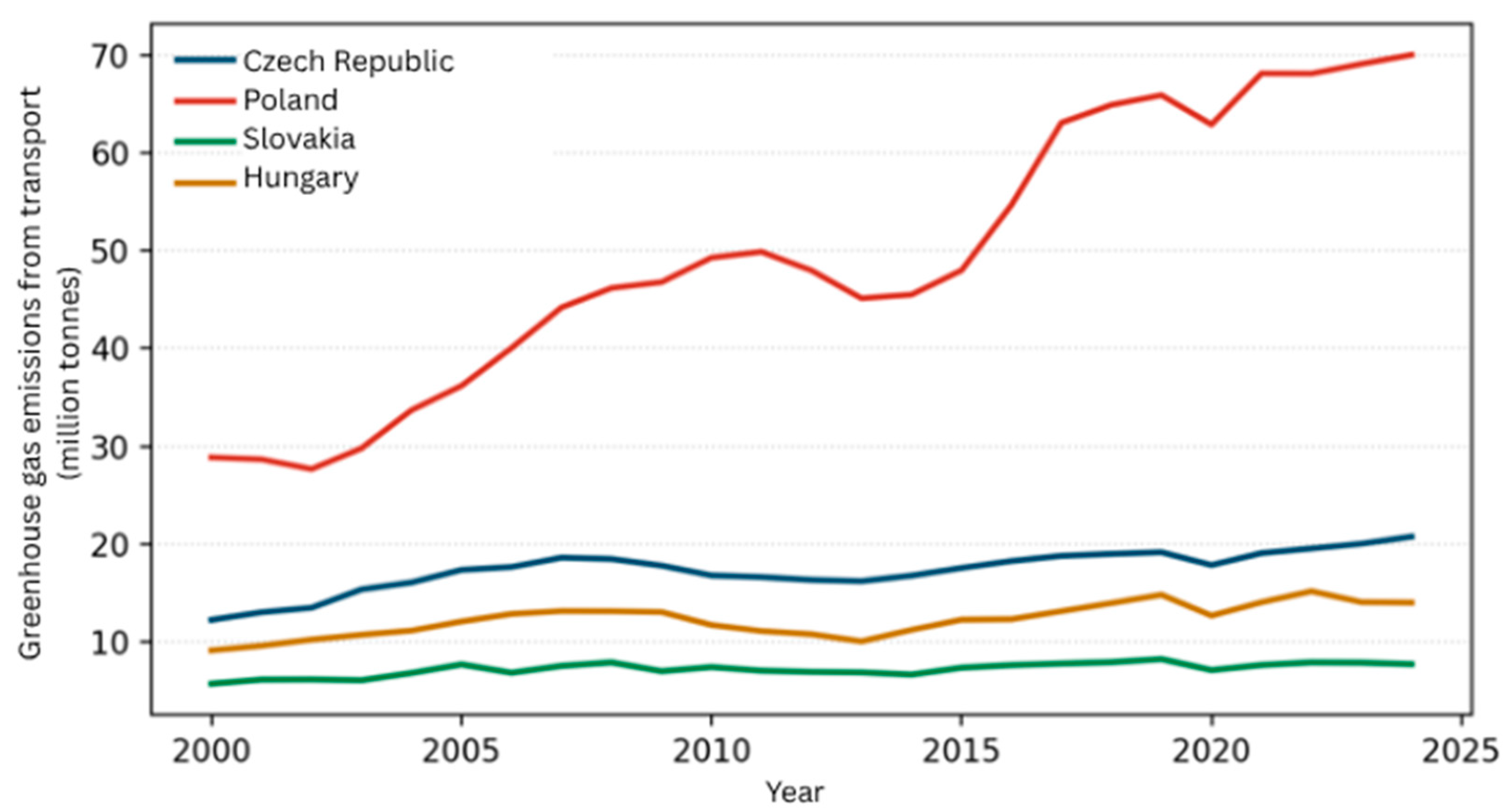
Figure 1 shows the development of greenhouse gas emissions from transportation in the Visegrad Group countries between 2000 and 2024. Poland recorded the highest emissions throughout the entire period under review, with emissions rising from approximately 29 million metric tons to 70 million metric tons. The growth was most pronounced after 2015, with only short-term declines recorded in 2013–2014 and 2020. The Czech Republic reported the second-highest emissions, which gradually increased from approximately 12 million metric tons to more than 20 million metric tons, with a relatively stable trend featuring a slight decline following the global financial crisis and in 2020. Hungary’s emissions ranged from approximately 9 to 15 million metric tons, with a decline from 2010 to 2013 followed by renewed growth. Slovakia reported the lowest emissions throughout the entire period, ranging from approximately 5.5 to 8 million metric tons, with a relatively stable trend. In all countries, a temporary reduction in emissions can be observed in 2020, likely due to transportation restrictions during the COVID-19 pandemic, followed by a return to an upward trend.

Table 1. Descriptive statistics for the variables (original units, n = 100).

Variable	Mean	Median	Std. Dev.	Min	Max	Skewness
GHG emissions from transportation (thousand metric tons)	21,539.4	14,058.5	17,983.6	5721.59	70,009.6	1.46
GDP per capita (EUR)	12,924.3	12,175.0	5600.7	4140.00	29,440.0	0.71
Length of highways and e-roads (km)	960.2	776.0	526.9	295.70	1897.0	0.40
Freight transport (tkm)	84,432.1	39,063.0	99,879.1	11,628.00	385,089.0	1.92
Environmental taxes (transportation)/GDP	0.0025	0.0023	0.0012	0.0002	0.0076	1.39
Renewable energy in transportation (%)	4.9	5.7	2.8	0.86	11.6	−0.15
Tax-to-freight intensity (EUR per million tkm)	7109.0	5414.6	4965.4	877.5	31,035.7	1.88

presents the basic descriptive characteristics of the analyzed variables. Average greenhouse gas emissions from transportation amounted to 21,539.4 thousand metric tons, while the high standard deviation (17,983.6 thousand metric tons) indicates significant differences among the V4 countries. Significant variability was also observed in the volume of freight transport, with an average value of 84,432.1 million ton-kilometers; the standard deviation (99,879.1) exceeded the average itself. This suggests a marked heterogeneity in the transport performance of the countries under review. Similarly, GDP per capita showed considerable differences, ranging from 4140 EUR to 29,440 EUR, reflecting the varying levels of economic development among the V4 countries.

The average length of highways and e-roads reached 960.2 km, with values ranging from 295.7 km to 1897 km. The average share of environmental taxes on transportation in GDP was 0.25%, while the share of renewable energy in transportation averaged 4.9%. The tax-to-freight intensity indicator had an average value of 7109.0 EUR per million tkm, with a range from 877.5 to 31,035.7 EUR per million tkm, indicating significant differences in the tax burden per unit of freight activity among individual countries.

A skewness analysis showed that freight transport volume exhibited the most pronounced right-skewed asymmetry (1.92), followed by greenhouse gas emissions from transportation (1.46) and the tax-to-freight intensity indicator (1.88). Right-skewed asymmetry was also present in the share of environmental taxes in GDP (1.39) and GDP per capita (0.71). In contrast, the length of the highway network (0.40) exhibited only mild asymmetry, and the share of renewable energy in transportation (−0.15) was distributed almost symmetrically. These results justify a logarithmic transformation of variables with more pronounced asymmetry prior to subsequent econometric analysis.

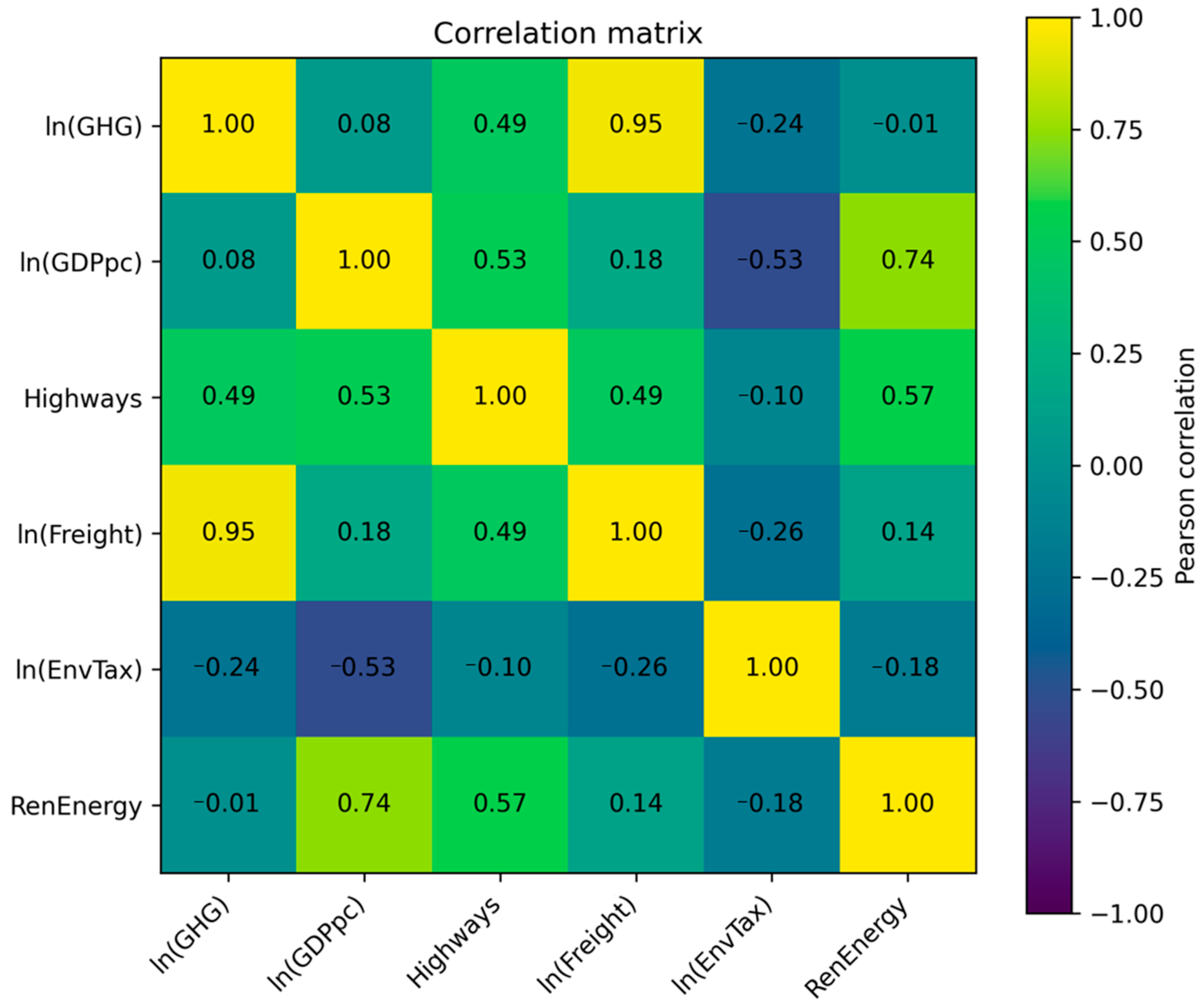
The results of the correlation matrix (Figure 2) show a very strong positive correlation between greenhouse gas emissions from transportation and the volume of freight traffic (r = 0.95), suggesting that growth in transportation volume is closely linked to an increase in emissions. Moderately strong positive relationships were found between emissions and the length of the highway network (r = 0.49), as well as between GDP per capita and the share of renewable energy in transportation (r = 0.74) and between GDP per capita and the length of highways (r = 0.53). Conversely, environmental taxes on transportation showed a negative correlation with GDP per capita (r = −0.53) and weaker negative relationships with emissions (r = −0.24) and the volume of freight transport (r = −0.26).

The correlation analysis does not indicate the presence of extremely high correlations among the explanatory variables (with the exception of the relationship between emissions and freight transport, which involves the dependent variable and is therefore not itself a multicollinearity concern). This was formally verified using Variance Inflation Factors (VIF), reported individually for each explanatory variable in

Table 2. Variance Inflation Factors for the explanatory variables in the baseline model.

Variable	VIF
ln(GDP per capita)	3.82
Length of highways and e-roads (km)	2.23
ln(Freight transport, tkm)	1.55
ln(Environmental taxes on transport/GDP)	1.86
Renewable energy in transportation (%)	2.75

. All values are well below the conventional threshold of 5, so the presence of problematic multicollinearity among the explanatory variables was not confirmed.

3.1. Model Selection: Pooled OLS, Fixed Effects, and Random Effects

To identify the appropriate panel specification, three basic models were estimated: the pooled OLS model, the fixed-effects (FE) model, and the random-effects (RE) model. The results of the individual estimates are presented in

Table 3. Comparison of Pooled OLS, Fixed Effects, and Random Effects estimates (basic model; standard errors in parentheses).

Variable	Pooled OLS b (SE)	Fixed Effects b (SE, Cluster)	Random Effects b (SE)
ln (GDP per capita)	−0.1040 (0.0730)	0.2440 (0.0989)	0.0943 (0.0565)
Length of highways and e-roads (km)	0.0003 (0.0000)	0.0001 (0.0001)	0.0001 (0.0000)
ln (Freight transport, tkm)	0.7093 (0.0240)	0.2304 (0.1196)	0.4441 (0.0458)
ln (Environmental taxes on transportation/GDP)	−0.0717 (0.0390)	0.0401 (0.0300)	−0.0154 (0.0335)
Renewable energy in transportation (%)	−0.0561 (0.0100)	−0.0293 (0.0072)	−0.0279 (0.0073)

. The coefficient estimates differed somewhat across models, particularly for the variables GDP per capita and freight transport, suggesting the existence of unobserved heterogeneity among the V4 countries.

The coefficients of the pooled OLS model systematically differ from the estimates of both the FE and RE specifications (e.g., the sign of ln (GDP per capita) and the magnitude of the coefficient for ln (freight transport)), which signals the presence of unobserved, time-invariant heterogeneity among the V4 countries (differences in energy mix, geographic location, industrial structure, or transport policy history), which the pooled data model does not account for. The F-test for the poolability of individual effects confirms this assumption: F(3, 91) = 114.10, p < 0.001, leading to an unequivocal rejection of the pooled data model in favor of the fixed-effects model.

The formal Hausman test comparing FE and RE estimates cannot be reliably interpreted in this case. With a very small number of cross-sectional units (N = 4 V4 countries), the difference covariance matrix of the FE and RE estimates is numerically close to singular, which, in the classical calculation of the test statistic, generates extreme, practically uninterpretable χ² values a well-known limitation of the Hausman test in “narrow but deep” panels with small N [26]. Instead of the formal Hausman test, the choice of specification was therefore based on (i) the F-test for poolability, which unequivocally rejects the pooled data model in favor of FE, and (ii) theoretical and substantive arguments: the V4 countries systematically differ in time-invariant, hard-to-measure characteristics (e.g., historical fleet structure, topography, location within European transport corridors) that are likely to correlate with the explanatory variables, thereby violating the key assumption of the random-effects model regarding the uncorrelatedness of individual effects with the regressors. The fixed-effects model is therefore chosen as the preferred baseline specification for all subsequent analyze.

3.2. Diagnostic Testing and Baseline Model

Before interpreting the coefficients, the basic assumptions of panel regression were tested. The Breusch–Pagan test for homoscedasticity rejected the null hypothesis of constant variance in the residuals (LM = 14.31; p = 0.014), indicating the presence of heteroscedasticity. The Wooldridge test for first-order autocorrelation indicated mild autocorrelation at the conventional 5% significance level (p = 0.055). Pesaran’s CD test for cross-sectional dependence did not reject the null hypothesis of independence of residuals across countries (CD = 1.591; p = 0.112), although given the small number of cross-sectional units (N = 4), this test has limited power. Given the indicated heteroscedasticity and marginal autocorrelation, all final models were estimated using Driscoll–Kraay robust standard errors (with Bartlett’s kernel and a 2 year lag, selected according to the Newey–West rule), which provide consistent estimates even in the presence of heteroscedasticity, autocorrelation, and cross-sectional dependence of the residuals.

Table 4. Base model (Fixed Effects, Driscoll–Kraay SE); n = 100.

Variable	Coefficient	DK SE	t-Stat.	p-Value
ln(GDP per capita)	0.2440 ***	0.0515	4.738	<0.001
Length of highways and e-roads (km)	0.0001 ***	0.0001	2.712	0.008
ln(Freight transport, tkm)	0.2304 ***	0.0483	4.772	<0.001
ln(Environmental taxes on transport/GDP)	0.0401	0.0244	1.645	0.103
Renewable energy in transportation (%)	−0.0293 ***	0.0084	−3.482	<0.001

Note: *** indicates statistical significance at the 1% level.

presents the results of the baseline model with fixed effects and Driscoll–Kraay standard errors. The model explains 83.0% of the variability in the logarithm of emissions within countries (within R²).

The elasticity of emissions with respect to GDP per capita is positive and highly statistically significant (b = 0.244; p < 0.001): a 1% increase in GDP per capita is associated with an increase in transportation emissions of approximately 0.24%, consistent with the expected positive association between economic activity and transportation emissions in economies that (unlike wealthier Western European economies) do not yet appear to have passed the inflection point of an environmental Kuznets curve for transport. The strongest predictor of emissions is the volume of freight transport (b = 0.230; p < 0.001), confirming its central role in the structure of V4 transportation emissions. The length of the highway and e-road network has a positive and statistically significant association with emissions (b = 0.00015; p = 0.008); expansion of the highway network during the period under review is thus associated more with an increase in motor vehicle traffic (an “induced demand” effect) than with a decrease. The share of renewable energy in transportation shows the expected negative and significant association with emissions (b = −0.0293; p < 0.001), consistent with a decarbonization effect. The coefficient for environmental taxes on transportation is positive in the baseline model but statistically insignificant (b = 0.0401; p = 0.103); an immediate association consistent with the “polluter pays” principle is therefore not confirmed in the baseline specification.

3.3. Robustness to Common Time Shocks: Two-Way Fixed Effects

The one-way (country) fixed-effects model does not by itself control for shocks common to all four countries in a given year.

Table 5. Two-way (country + year) Fixed Effects model, Driscoll–Kraay SE; n = 100.

Variable	Coefficient	DK SE	t-Stat.	p-Value
ln(GDP per capita)	0.0673	0.1539	0.437	0.663
Length of highways and e-roads (km)	0.0001	0.0001	1.525	0.132
ln(Freight transport, tkm)	0.2697 ***	0.0471	5.722	<0.001
ln(Environmental taxes on transport/GDP)	0.0169	0.0279	0.603	0.548
Renewable energy in transportation (%)	−0.0214	0.0154	−1.391	0.169

Note: *** indicate statistical significance at the 1% level.

reports the same baseline specification re-estimated with a full set of year dummies added to the country fixed effects. An F-test comparing this two-way specification to the one-way model confirms that the year effects are jointly statistically significant: F(24, 67) = 1.788, p = 0.033, indicating that common, economy-wide shocks (the 2008–2009 financial crisis, the 2020 COVID-19 mobility restrictions, and post-2021 energy-price movements, among others) explain a statistically meaningful share of year-to-year variation in transport emissions beyond what the five structural regressors capture.

The two-way specification changes the substantive picture in an important way. The within R² falls from 0.830 in the one-way model to 0.606 once year effects are added—consistent with a meaningful share of the one-way model’s explanatory power coming from trends common to all four countries rather than from country-specific variation in the regressors. Freight transport volume remains highly significant and of similar magnitude (b = 0.270; p < 0.001), confirming it as the most robust driver of transport emissions in the V4 sample regardless of specification. By contrast, GDP per capita (b = 0.067; p = 0.663) and the share of renewable energy (b = −0.0214; p = 0.169) both lose statistical significance once common year effects are controlled for, and the length of the highway network is only marginally significant (p = 0.132). The coefficient on environmental taxes remains small and statistically insignificant in both specifications (one-way: b = 0.040, p = 0.103; two-way: b = 0.017, p = 0.548).

We interpret this pattern cautiously rather than as a wholesale reversal of the baseline findings. GDP per capita and the renewable-energy share both moved in broadly similar directions across all four V4 countries over 2000–2024 (steady income convergence toward the EU average; a shared, EU-driven expansion of biofuel blending mandates and renewable-transport targets under sequential EU renewable-energy directives). Year fixed effects will, by construction, absorb exactly this kind of common trend, which can legitimately reduce the precision (and, here, the significance) of coefficients on regressors that move together with the absorbed trend, without necessarily implying that the underlying relationship is spurious. 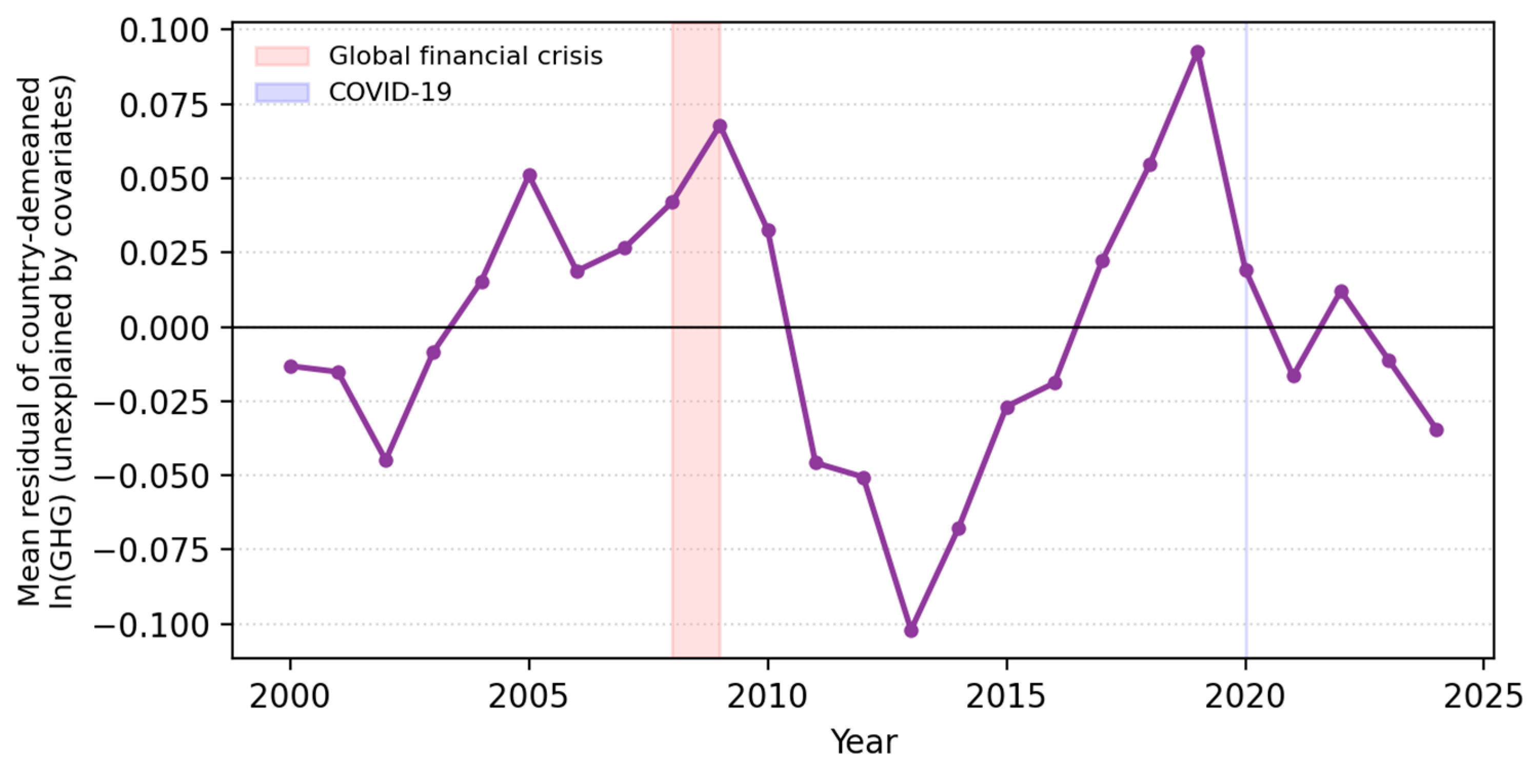Figure 3 illustrates the common time pattern being absorbed: it plots the average within-country residual (from the one-way FE model) by year, which is systematically below trend in 2011–2014 and above trend in 2017–2019, consistent with the EU-wide post-crisis contraction and the subsequent recovery in freight activity, and only mildly affected in 2020 once GDP and freight (which themselves fell sharply that year) are already controlled for. Given this evidence, we treat the freight-transport finding as the most robust result of this study, and we treat the GDP per capita and renewable-energy findings as robust within-country associations that should nonetheless be read together with the possibility that part of their apparent effect reflects shared regional trends.

All lag, interaction, and robustness analyses use the one-way (country) fixed-effects specification as the baseline, consistent with the sequential model-building strategy described in Section 2.2 and given that adding both year dummies and multiple lag or interaction terms simultaneously would leave very few residual degrees of freedom at N = 4. Where relevant, we note whether a given result also survives in the corresponding two-way specification.

3.4. Lagged Effects of Environmental Taxes

To verify whether the association of environmental taxes on transportation manifests itself with a time lag, the baseline model was expanded to include one-year, two-year, and three-year lags (lag 1–lag 3) of the logarithm of the variable “Environmental tax revenues (Transport taxes)/GDP.” In accordance with the recommendation not to include lags of multiple variables simultaneously in a single model (given the limited number of degrees of freedom at N = 4), only environmental tax lags were included in this specification. Using the lags, the sample was reduced to n = 88 observations. The results are presented in

Table 6. Model with lags in environmental taxes (Fixed Effects, Driscoll–Kraay SE); n = 88.

Variable	Coefficient	DK SE	t-Stat.	p-Value
ln(GDP per capita)	0.2871 ***	0.0689	4.169	<0.001
Length of highways and e-roads (km)	0.0001 **	0.0001	2.059	0.043
ln(Freight transport, tkm)	0.2000 ***	0.0495	4.038	<0.001
ln(Environmental taxes on transport/GDP)	0.0342	0.0316	1.084	0.282
ln(Environmental taxes), lag 1	0.0055	0.0215	0.254	0.800
ln(Environmental taxes), lag 2	0.0322	0.0273	1.179	0.242
ln(Environmental taxes), lag 3	0.0140	0.0338	0.414	0.680
Renewable energy in transportation (%)	−0.0274 ***	0.0075	−3.630	<0.001

Note: **/*** indicates statistical significance at the 5%/1% level.

.

Neither the current level of environmental taxes nor any of the three lags (lag 1: b = 0.0055, p = 0.800; lag 2: b = 0.0322, p = 0.242; lag 3: b = 0.0140, p = 0.680) reach statistical significance at the usual significance levels. The hypothesis of a delayed effect of tax policy on greenhouse gas emissions from transportation is therefore not confirmed in this sample of V4 countries, either because the tax incentives are too small in absolute terms to induce a measurable change in the behavior of the transportation sector even after a three-year lag, or because the short panel (25 years, 4 countries) does not provide sufficient statistical power to detect a gradually emerging effect. The other variables retain the expected signs and approximate magnitudes of the coefficients as in the baseline model.

3.5. Lagged Effects of Renewable Energy

In a similar manner, the baseline model was expanded to include one- to three-year lags in the share of renewable energy in transportation to verify whether the decarbonization effect of these variable manifests itself gradually (

Table 7. Model with lags in renewable energy (Fixed Effects, Driscoll–Kraay SE); n = 88.

Variable	Coefficient	DK SE	t-Stat.	p-Value
ln (GDP per capita)	0.3299 ***	0.0658	5.013	<0.001
Length of highways and e-roads (km)	0.0002 ***	0.0000	4.189	<0.001
ln (Freight transport, tkm)	0.1833 ***	0.0408	4.493	<0.001
ln (Environmental taxes on transportation/GDP)	0.0434 *	0.0236	1.838	0.070
Renewable energy in transportation (%)	−0.0129 *	0.0068	−1.893	0.062
Renewable energy, lag 1	−0.0108 **	0.0054	−2.009	0.048
Renewable energy, lag 2	−0.0061	0.0060	−1.026	0.308
Renewable energy, lag 3	−0.0126 *	0.0073	−1.733	0.087

Note: */**/*** indicates statistical significance at the 10%/5%/1% level.

).

Unlike environmental taxes, there is some evidence of a lag effect for renewable energy: both the present value (b = −0.0129, p = 0.062) and its first lag (b = −0.0108, p = 0.048) are statistically significant at the 10% and 5% levels, respectively, with the same negative sign, while the third lag is significant at the 10% level (b = −0.0126, p = 0.087) and the second lag is not significant (p = 0.308). Taking together, this suggests that expanding the use of renewable energy sources in transportation reduces greenhouse gas emissions not only immediately, but this effect may persist (albeit with lower estimation precision) for up to three years, which is consistent with the gradual renewal of the vehicle fleet and infrastructure for alternative fuels.

3.6. Moderating Effect of Transport Infrastructure

To verify whether the associations of environmental taxes depends on the level of development of the transportation infrastructure, the basic model was expanded to include an interaction term between the logarithm of environmental taxes and the length of the highway and e-road networks (

Table 8. Interaction model: environmental taxes × length of highway network (Fixed Effects, Driscoll–Kraay SE); n = 100.

Variable	Coefficient	DK SE	t-Stat.	p-Value
ln (GDP per capita)	0.2289 ***	0.0495	4.625	<0.001
Length of highways and e-roads (km)	−0.0003	0.0003	−1.145	0.255
ln (Freight transport, tkm)	0.2230 ***	0.0453	4.924	<0.001
ln (Environmental taxes on transportation/GDP)	0.1563 **	0.0698	2.239	0.028
Renewable energy in transportation (%)	−0.0256 ***	0.0091	−2.826	0.006
ln (Environmental taxes) × Length of highways	−0.0001	0.0000	−1.641	0.104

Note: **/*** indicates statistical significance at the 5%/1% level.

).

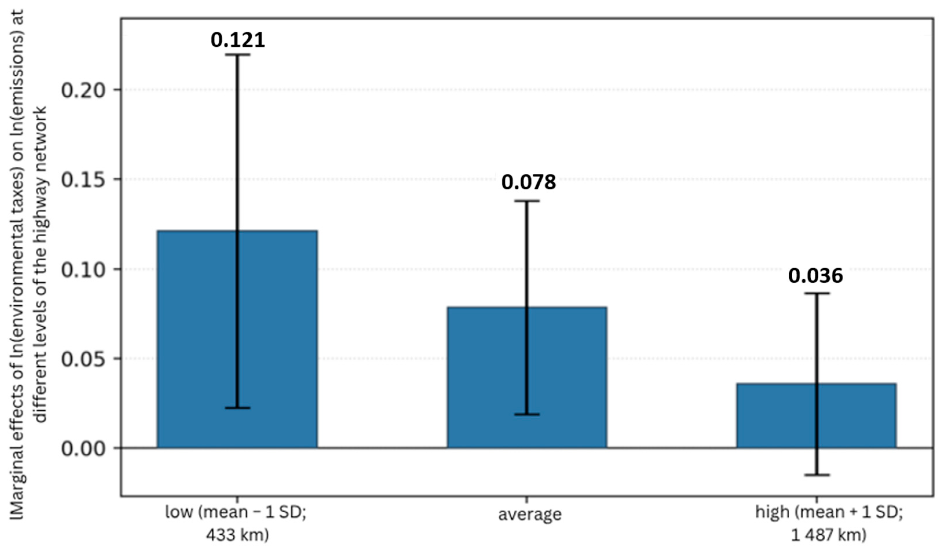
In the interaction model, the main association of environmental taxes is positive and statistically significant (b = 0.156; p = 0.028), while the interaction term is negative, albeit only at the 10% significance level (b = −0.00010; p = 0.104). The negative sign of the interaction indicates that the relationship between environmental taxes and emissions weakens as the length of the highway network increases. Since the interaction coefficient alone is not very meaningful in terms of interpretation, the marginal effects of environmental taxes on emissions were calculated at low (mean − 1 SD), medium, and high (mean + 1 SD) levels of highway network length (

Table 9. Marginal effects of ln (environmental taxes) on ln(emissions) at different levels of the highway network.

The Extent of the Highway Network	∂ ln (GHG)/∂ln (EnvTax)	SE	z-Stat.	p-Value
low (mean − 1 SD; 433 km)	0.1211	0.0503	2.408	0.016
average (960 km)	0.0784	0.0304	2.582	0.010
high (mean + 1 SD; 1487 km)	0.0357	0.0258	1.383	0.167

, Figure 4).

The marginal effect of environmental taxes is statistically significant and strongest in countries/years with a below-average motorway network (∂ln(GHG)/∂ln(EnvTax) = 0.121; p = 0.016), decreases at the average infrastructure level (0.078; p = 0.010), and loses statistical significance for highly developed highway networks (0.036; p = 0.167). It should be emphasized that in all three cases the estimated direction of the association is positive, i.e., higher environmental taxes in this sample are associated with higher, not lower, emissions. This likely reflects an endogenous, mechanical link between the volume of taxed transportation activity and the level of collected environmental taxes (a higher volume of transportation generates both higher emissions and higher tax revenue from fuel consumption), rather than a causal reduction effect of taxation. Nevertheless, the finding most relevant to this study’s research question is that this (positive) association is strongest precisely where highway infrastructure is least developed, and disappears, in a statistical sense, where the network is more developed: transport infrastructure moderates the strength, though not the overall sign, of the relationship between environmental taxation and transport emissions in this sample.

3.7. Robustness Check: Tax-to-Freight Intensity

To verify the stability of the results, the baseline model was re-estimated by replacing the variable “Environmental tax revenues (Transport taxes)/GDP” with the tax-to-freight intensity indicator (environmental tax revenue on transportation per unit of freight transport volume, rather than per unit of GDP), which reflects the level of taxation relative to the transport activity most directly responsible for emissions while avoiding division by the dependent variable itself (

Table 10. Robustness model with the tax-to-freight intensity variable (Fixed Effects, Driscoll–Kraay SE); n = 100.

Variable	Coefficient	DK SE	t-Stat.	p-Value
ln(GDP per capita)	0.2028 ***	0.0428	4.744	<0.001
Length of highways and e-roads (km)	0.0001 ***	0.0001	2.692	0.008
ln(Freight transport, tkm)	0.2715 ***	0.0372	7.293	<0.001
ln(Tax-to-freight intensity)	0.0414 *	0.0249	1.664	0.100
Renewable energy in transportation (%)	−0.0294 ***	0.0085	−3.476	<0.001

Note: */*** indicates statistical significance at the 10%/1% level.

).

Diagnostic tests of the robustness model show a broadly similar pattern to the baseline model: the Breusch–Pagan test again indicates heteroscedasticity (LM = 13.92; p = 0.016), the Wooldridge test suggests mild autocorrelation (p = 0.055), and the Pesaran CD test does not reject cross-sectional independence in this specification (CD = 1.585; p = 0.113), consistent with the continued use of Driscoll–Kraay standard errors. The coefficients for GDP per capita, freight transport, and renewable energy remain consistent with the baseline model in both sign and approximate magnitude, supporting the overall robustness of these findings. The coefficient for the tax-to-freight intensity indicator is positive, mirroring the baseline model’s environmental-tax coefficient, and is significant only at the 10% level (b = 0.0414; p = 0.100)—weaker than the (insignificant) baseline result, but in the same, theoretically unexpected direction.

The robustness model was further extended to include one-, two-, and three-year lags of the tax-to-freight intensity indicator; using the lagged variables reduced the sample to n = 88 observations (

Table 11. Robustness model with lags of the tax-to-freight intensity variable (Fixed Effects, Driscoll–Kraay SE); n = 88.

Variable	Coefficient	DK SE	t-Stat.	p-Value
ln(GDP per capita)	0.2413 ***	0.0600	4.018	<0.001
Length of highways and e-roads (km)	0.0001	0.0001	1.321	0.191
ln(Freight transport, tkm)	0.2526 ***	0.0427	5.909	<0.001
ln(Tax-to-freight intensity)	0.0345	0.0275	1.251	0.215
ln(Tax-to-freight intensity), lag 1	0.0107	0.0215	0.499	0.619
ln(Tax-to-freight intensity), lag 2	0.0172	0.0206	0.835	0.407
ln(Tax-to-freight intensity), lag 3	−0.0888 **	0.0378	−2.353	0.021
Renewable energy in transportation (%)	−0.0253 ***	0.0082	−3.080	0.003

Note: **/*** indicates statistical significance at the 5%/1% level.

).

Neither the current value of the indicator nor its first- or second-order lags show a statistically significant association with emissions (current: p = 0.215; lag 1: p = 0.619; lag 2: p = 0.407). Only the third lag is statistically significant and negative (b = −0.0888; p = 0.021), a pattern that mirrors, at face value, the result obtained with the earlier emissions-denominated indicator.

3.8. Sensitivity Check: Does the Three-Year Lag Reflect a Mechanical Artifact?

Unlike the emissions-denominated indicator used in the original submission, the tax-to-freight intensity indicator does not divide by the dependent variable: its denominator is freight transport volume, a control variable already included, at its contemporaneous value, in every specification reported in this study (Table 3, Table 4, Table 5, Table 6, Table 7, Table 8, Table 9 and Table 10). This construction removes the direct algebraic channel identified in Section 2.2 (whereby ln(GHG)_it−3 mechanically appears inside a GHG-denominated regressor and re-enters the regression through the strong own-persistence of emissions). However, because freight transport is itself highly correlated with emissions (r = 0.95 contemporaneously) and moderately persistent over time (three-year within-country autocorrelation of ln(freight) = 0.68), a weaker, indirect version of the same concern could in principle remain: lagged freight, embedded in the lagged tax-to-freight regressor, might still proxy for emissions dynamics not captured by the contemporaneous freight term already in the model.

We tested this directly by regressing the within-country residual of ln(GHG) after removing the part explained by contemporaneous freight transport, exactly as freight enters every specification in this study on the three-year lag of ln(freight) (the term mechanically embedded in the lagged tax-to-freight regressor). The resulting correlation is 0.083, essentially negligible, and dramatically smaller than the equivalent check for the original emissions-denominated indicator, where current and third-lagged log-emissions were correlated at −0.988. In other words, once contemporaneous freight transport is controlled for, as it always is in this study, lagged freight carries almost no additional mechanical information about current emissions.

This does not, on its own, prove that the three-year lag reported in Table 11 reflects a genuine, delayed association of taxation: it remains the only significant result among the lags tested for this indicator (as for the GDP-denominated tax variable in Table 6 and the renewable-energy variable in Table 7), and with N = 4 countries some caution against over-interpreting any single coefficient, however constructed, remains warranted. But because the mechanical channel that motivated this sensitivity check in the first place is now shown to be negligible, we treat this result differently from the earlier, emissions-denominated version: rather than dismissing it as a likely artifact, we report it as a tentative, non-mechanical finding consistent with a delayed association between transport taxation intensity and emissions, to be corroborated in future work with a longer panel.

3.9. Summary of Results

The results of the panel analysis of the V4 countries for 2000–2024 can be summarized in six points:

• Model selection: The F-test for poolability unequivocally rejects the pooled data model in favor of the fixed-effects model (F = 114.1; p < 0.001); the formal Hausman test is not reliably interpretable at N = 4, so the choice of the FE model is additionally supported by theoretical arguments regarding unobserved heterogeneity among the V4 countries.
• Determinants of emissions: Greenhouse gas emissions from transportation are most strongly and consistently associated with the volume of freight transport (elasticity 0.23) and, in the one-way FE model, with GDP per capita (elasticity 0.24), while the share of renewable energy in transportation shows a reducing association (b = −0.029). Freight transport is the only one of these three that remains significant once common year effects are controlled for (Point 6 below).
• Lag effects: The hypothesis of a lagged association between environmental taxes (relative to GDP) and emissions (H3) was not confirmed at any of the tested lags; the association between renewable energy and emissions shows signs of persisting for up to three years (partial support for H2).
• Moderating effect of infrastructure: The (positive) association between environmental taxes and emissions is strongest where highway networks are less developed and loses statistical significance where the network is highly developed—consistent with H4, although the underlying interaction term is only marginally significant (p = 0.104), so this should be read as preliminary support pending a dedicated formal test of moderation.
• Robustness: Replacing environmental taxes (relative to GDP) with the tax-to-freight intensity indicator (relative to freight activity) yields a smaller, only marginally significant positive coefficient at the current level and no significant association at one- or two-year lags; a significant, negative three-year lag is present, and unlike the equivalent result under the original emissions-denominated indicator a dedicated sensitivity check (Section 3.8) finds no meaningful mechanical channel behind it. Because this is the only significant lag among several tested for this indicator, it is best read as exploratory rather than confirmatory evidence; taken together with the GDP-denominated result, it is consistent with H5’s claim that the tax–emissions association is sensitive to how tax intensity is operationalized.
• Common time shocks: A two-way (country + year) fixed-effects specification shows that year effects are jointly significant (F(24, 67) = 1.79, p = 0.033); once these are controlled for, freight transport remains a robust driver of emissions, but the GDP per capita and renewable-energy associations lose statistical significance, suggesting that part of their apparent effect in the baseline model reflects trends common to all four countries rather than purely country-specific variation.

The results suggest that in the V4 countries, the volume of economic and freight activity remains the main correlate of greenhouse gas emissions from transportation, while the direct, short-term association between environmental taxation on transportation and emissions is weak and sensitive to the choice of denominator; a longer-horizon association is more defensible once the tax indicator is measured relative to freight activity rather than to emissions themselves. The association between renewable energy sources and lower emissions appears more consistent and, to some extent, persistent over time, though not entirely independent of common regional trends. Given the observational panel design, the small number of cross-sectional units, and the endogeneity concerns discussed in Section 2.3, all of the above should be read as descriptive associations rather than as definitive causal effects.

4. Discussion

This section places the six results summarized in Section 3.9 in the context of recent (2020–2025) peer-reviewed literature, distinguishes genuine substantive disagreement from differences attributable to measurement choices, and draws out the implications for logistics operators, policymakers, and future research. To keep this discussion focused and to avoid repeating material already presented in Section 3, each subsection states the finding briefly before turning to its interpretation.

4.1. Freight Transport and Economic Growth as the Main Drivers of Emissions

The finding that freight transport volume (elasticity 0.23) and, in the one-way FE model, GDP per capita (elasticity 0.24) are the strongest predictors of transport emissions is consistent with most of the current literature. In a panel of EU countries, freight-transport infrastructure development has been shown to directly increase CO₂ emissions [27], and in a sample of OECD countries, growth in transport activity is estimated to increase transport emissions by an average of up to 46.45% [28]. A comprehensive global review of emissions trends identifies road freight transport as the main source of growth in sectoral emissions precisely because freight volume grows in tandem with GDP [1]—exactly the mechanism our estimate captures. Similarly, a positive association between GDP per capita and transportation emissions has been documented in China [17] and among the five most populous countries in the world [29]. Our finding is thus consistent with the broader international pattern in which the V4 countries, over 2000–2024, had not yet reached the inflection point of an environmental Kuznets curve for transport, unlike more developed Western European economies where a relative or absolute decline in transportation emissions has already been observed alongside rising income.

Turkey is a documented exception to this pattern: both road and rail freight transport were found to reduce emissions there [30], a result attributed to fleet modernization, increased logistical efficiency, and infrastructure development enabling a shift toward less emission-intensive transport modes. This exception is instructive: the positive association between freight volume and emissions is not deterministic but depends on the technological level of the vehicle fleet and on whether growth in transport volume is accompanied by efficiency gains. Because our model does not include a direct indicator of V4 fleet technological sophistication, part of the positive freight coefficient may reflect this omitted channel; disaggregated fleet-age and Euro-emission-standard data, where available, would be a natural addition in future work.

The GDP per capita association weakens and loses statistical significance once year fixed effects are added, which we interpret as evidence that a meaningful part of its apparent effect in the baseline model reflects the shared, EU-wide income-convergence trend across the four V4 countries during this period rather than a purely country-specific relationship. This does not contradict the broader literature cited above, which is itself typically estimated on much larger, more heterogeneous panels where common trends are less dominant relative to cross-sectional variation but it does mean that our GDP finding should be read as a within-country association net of that trend, rather than as an independently identified elasticity.

4.2. Renewable Energy: The Most Robust Decarbonization Channel

The statistically significant reducing association between the share of renewable energy in transportation and emissions (b = −0.0293; p < 0.001) is among the most consistently confirmed findings of this study relative to literature. In the U.S., renewable-energy use in transportation has been shown to mitigate CO₂ emissions and, in a Granger-causal sense, to precede their decline [31]. In European countries, higher renewable-energy consumption is estimated to reduce transportation emissions by approximately 12% [32], broadly consistent with both direction and magnitude of our estimate. A panel analysis of EU countries for 2007–2020 confirmed that higher renewable-energy adoption is associated with a decline in transportation emissions [4], and the same direction of association has been observed for the G7 [33] and for China [17]; this pattern extends to the BICS group of countries [34] and to so-called energy-transition countries [35].

The consistency of this result across such a diverse sample of countries (the U.S., the EU, China, the G7, and BICS) reinforces confidence that the decarbonization association between renewable energy and transport emissions is not specific to the V4 context but represents a broad, largely general pattern. Our analysis adds to this literature by documenting a partially persistent lag structure that this mostly cross-sectional and short-panel literature generally does not examine, while also showing that some of this persistence should be interpreted net of a shared regional adoption trend rather than as a purely country-specific effect.

The persistence of the renewable-energy effect over one to three years can also be interpreted through the adjustment dynamics of the transport sector. Changes in the renewable-energy share do not immediately translate into lower emissions because freight operators typically renew their vehicle fleets gradually, while investments in charging infrastructure, alternative-fuel facilities, and related energy systems are implemented over multi-year investment cycles. As cleaner vehicles and supporting infrastructure become progressively available, the initial increase in renewable-energy use may therefore generate a cumulative rather than instantaneous reduction in transport emissions. This mechanism is particularly relevant in freight transport, where capital-intensive vehicle replacement and infrastructure constraints slow down short-run adjustment. This interpretation is consistent with the lag structure observed in our estimates, although the effect should be interpreted cautiously because part of the persistence may also reflect common regional trends in renewable-energy adoption.

4.3. Why Did We Not Find a Robust Tax Effect? Instrument Heterogeneity and Tax Incidence

The most notable discrepancy between our results and part of the literature concerns environmental taxes. While the coefficient for environmental taxes on transportation is statistically insignificant in our baseline model (b = 0.0401; p = 0.103) and even positive and significant in the interaction model (b = 0.156; p = 0.028), a panel study of European countries found transportation taxes to be negatively and significantly associated with CO₂ [7], and environmental taxes have been reported to reduce transport emissions in the BICS [34] and EU25 [36] country groups, although in the EU25 case the effect is primarily short-term.

Our null or counterintuitive result is nonetheless not isolated in the literature, and the conceptual distinctions drawn in Section 1.1 help explain why. A recent European study distinguishing between transport modes found that energy and transportation taxes have no long-term association with water-transport emissions, while only so-called pollution taxes reduce emissions from road and air transport [37], i.e., the effectiveness of taxation depends heavily on the specific type of tax and mode of transport, which vary across studies. Similarly, in China, although total environmental taxes sometimes reduce emissions, taxes on vehicles and vessels (the closest equivalent to our “environmental taxes on transport” indicator) are either ineffective or even counterproductive with respect to emission intensity [38]. This instrument-type heterogeneity is likely central to understanding our result, the Eurostat “Environmental tax revenues (Transport taxes)/GDP” indicator we use is, by construction, closer to narrowly defined fuel-excise and vehicle taxation than to a genuine Pigouvian carbon price, and it is precisely this category of tax for which the literature is least consistent in finding a reduction effect.

The economic mechanism that may underlie our (positive) result is illuminated by the tax-incidence literature in freight transport. In the U.S. truckload market, demand for freight transport has been shown to be inelastic in the short run, so that fuel and transportation taxes are passed through the supply chain to shippers and can even be “over-shifted” [39] that is, a tax increase shows up in higher freight rates without a corresponding decrease in freight volume (and hence in emissions). It has also been noted that in road transport there is only a weak alignment between the structure of fuel taxes and actual externalities, particularly congestion, meaning the current tax system is not efficiently targeted at emissions [40]. These findings are consistent with our observation that higher environmental taxes on transportation in our sample are not accompanied by a decrease, but rather by an increase (or no change), in emissions: if transport volume does not fall in the short run and the tax is largely passed through to prices and higher tax revenue, then the observed (positive) correlation between tax revenue and emissions may reflect exactly this endogenous link via the volume of taxed activity the mechanism flagged as a data-availability limitation for IV identification in Section 2.3 rather than an actual causal (non-)effect of the tax itself. It should also be noted that environmental taxes alone represent only one, relatively small, component of total transportation costs alongside tolls, VAT, purchase price, and infrastructure [41,42], which further limits their independent influence on carriers’ behavior. By contrast, for Latvia the opposite a reduction in transport emissions associated with environmental taxes has been reported [9], underscoring that these results are also sensitive to the specific country and institutional context of taxation.

4.4. Moderating Effect of Transport Infrastructure

The finding that the (positive) association between environmental taxes and emissions is strongest where highway networks are least developed and loses significance where the network is well developed has no exact counterpart in the reviewed literature; no identified study tests precisely this “transport infrastructure × environmental taxes” interaction. Several studies nonetheless indirectly support the idea that infrastructure moderates emission effects, more often through a technological-innovation channel than through tax policy. Transportation infrastructure alone has been shown to increase emissions, but in combination with technological innovation this effect weakens or reverses [27], i.e., infrastructure does not have a one-directional effect on its own; its net effect depends on accompanying factors, just as in our case it depends on the combination with tax policy. By contrast, in a panel of 12 European countries, no significant independent effect of transport-infrastructure investment on transport CO₂ was found [43], which undermines the notion of a universal infrastructure effect and is consistent with our finding that highway-network length alone has a statistically insignificant direct coefficient in the interaction specification. For the United States [31] and the five most populous countries in the world [29], road-infrastructure development was, on the contrary, found to increase emissions, in line with our baseline-model finding of an induced-demand effect. The combination of these findings suggests that the direction and strength of the infrastructure effect are highly context-dependent, making our documentation of a specific moderating mechanism between infrastructure and environmental taxation, in the V4 context, a potentially original contribution to the literature.

4.5. Sensitivity to Measurement, Lag Structure, and the Mechanical-Endogeneity Caveat

Our finding that replacing the “Environmental tax revenues (Transport taxes)/GDP” indicator with the alternative tax-to-freight intensity indicator weakens the estimated coefficient (from a fully insignificant b = 0.0401 to a marginally significant b = 0.0414, p = 0.100), while its sign remains positive rather than the theoretically expected negative, is directly consistent with evidence that the choice of a specific tax indicator (energy tax, transport tax, or pollution tax) fundamentally alters the estimated relationship to emissions by mode of transport [37]. Our study thus reinforces this more general conclusion: findings on the effectiveness of environmental taxation of transport are sensitive to how the tax variable is operationalized, so it is not meaningful to speak of a single, universal effect of an “emissions tax” without specifying the tax type and tax base in question.

The statistically significant three-year lag for tax-to-freight intensity (b = −0.0888, p = 0.021) is, unlike the equivalent result under the earlier emissions-denominated indicator, not attributable to a detectable mechanical channel: the residual correlation between current emissions (net of contemporaneous freight) and lagged freight is negligible (0.083), in sharp contrast to the near-unity correlation (−0.988) that undermined the equivalent check for the emissions-denominated version. Because this three-year lag is the only statistically significant tax-intensity lag among the several lag specifications tested across this study, it should be interpreted as exploratory rather than confirmatory evidence of a delayed taxation effect: with multiple coefficients tested across several tables, an isolated result at conventional significance levels is not strong evidence on its own, and we do not adjust for multiple comparisons given the exploratory nature of the lag analysis. We nonetheless treat this single, longer-lag finding with due caution given N = 4, and it is directly consistent with one indirect parallel in the literature: in China, an Environmental Protection Tax Law that does not directly tax CO₂ has been found to increase the synergistic reduction in SO₂, CO₂, and PM emissions [44], suggesting that broader regulatory “polluter pays” signals can, in principle, affect emissions indirectly and with a lag through channels such as fleet renewal or investment decisions. Corroborating this specific finding with a longer time series is a natural next step.

4.6. A Logistics-Operator Perspective: Routing, Modal Choice, and the NIMBY Constraint on Infrastructure-Led Solutions

Reading the tax-ineffectiveness and infrastructure-moderation findings through a logistics-operator lens helps reconcile them with operational reality. For a freight forwarder or carrier planning shipments along a V4 corridor, an environmental tax on transport is one of several largely fixed cost items, tolls, driver wages, fuel, vehicle depreciation that are set at the network or corridor level rather than the individual shipment level, and that are, in the short run, largely non-discretionary given contracted delivery windows and limited access to alternative modes on many V4 routes. Modal shift to rail or inland waterway, the channel through which taxation is theoretically supposed to reduce emissions [5], requires terminal access, compatible loading units, and schedule reliability that are unevenly available across the region; where highway infrastructure is sparse, road often remains the only realistic option regardless of its relative tax burden, which is consistent with our finding that the tax–emissions association is strongest precisely where the highway network is least developed, not because taxation “works less well” there in a policy-design sense, but because operators there have the least ability to substitute away from road freight in response to a price signal.

This operational constraint also connects to a distinct political-economy limitation on infrastructure-led decarbonization strategies that the literature on transport policy has increasingly highlighted: local opposition to the siting of new transport infrastructure, alternative-fuel facilities, or public-transport corridors, sometimes summarized as a “not in my back yard” (NIMBY) response. Even where residents broadly support the environmental rationale for decarbonizing freight transport and accept the logic of an emissions-related tax in the abstract, they may still oppose the concrete local siting of the new highway capacity, rail terminals, hydrogen refueling stations, or logistics hubs that would be needed to give carriers a realistic alternative to road transport, particularly in or near urban and residential zones. Because our data cannot separately identify siting opposition or permitting delays, we cannot test this mechanism directly; however, it offers a plausible complementary explanation for why the moderating effect of infrastructure documented in Section 3.6 may take years or decades to materialize in practice even where it is, in principle, part of an effective policy mix, and we flag NIMBY-related permitting and siting frictions as a concrete avenue for future V4-specific research.

4.7. Time and Place: When and Where Do These Associations Hold?

The results reported in Section 3 and Section 4.1, Section 4.2, Section 4.3, Section 4.4, Section 4.5 and Section 4.6 are pooled across 25 years and four countries, which can obscure meaningful variation in when and where each association is strongest. Two complementary pieces of evidence, both already presented, allow a first look at this variation without over-extending the model given N = 4.

On the time dimension, shows that the average within-country residual of ln(GHG), i.e., the part of emissions not explained by GDP, freight, infrastructure, taxation, or renewable energy was systematically below trend in 2011–2014 and above trend in 2017–2019, with only a mild, temporary dip around 2020. The 2011–2014 period corresponds to the sovereign-debt-crisis-era slowdown in the euro area, which depressed export demand for V4 manufacturing and freight activity beyond what contemporaneous GDP and freight figures alone capture; the 2017–2019 period corresponds to a strong, broad-based upswing in V4 export volumes and freight activity ahead of the COVID-19 shock. The comparatively muted 2020 residual is consistent with the fact that GDP per capita and freight transport volume themselves fell sharply that year and are already included as regressors, so much of the COVID-19 effect on emissions is captured through those variables rather than showing up as an additional, unexplained residual. This time-varying pattern reinforces the case, made methodologically in Section 2.1 and empirically in Section 3.3, for treating the one-way FE estimates of GDP per capita and renewable energy with some caution.

On the place dimension, shows that Poland’s transport emissions are three to four times larger in absolute terms than those of the other three V4 countries throughout the period, and that Poland alone accounts for most of the region’s post-2015 emissions growth, consistent with its larger economy, coal-dependent energy mix, and expanding road-freight sector. Czechia and Hungary show more moderate, comparatively steady growth, while Slovakia the smallest and most trade-integrated of the four economies, with a transport sector heavily oriented around automotive-supply-chain logistics shows the flattest trajectory. Because our fixed-effects specification nets out exactly this kind of time-invariant, country-level heterogeneity, none of the elasticities reported in Section 3 should be read as applying uniformly to, say, Poland’s coal-and-road-freight-heavy transport sector and Slovakia’s automotive-export corridor economy in the same way; the pooled elasticity is best interpreted as an average association across these differing structural contexts rather than as a description of any single country. A full country-by-country or sub-period re-estimation is not feasible with N = 4 (it would leave at most one cross-sectional unit per group), but we flag this heterogeneity explicitly as a direction for future research using a larger panel of Central and Eastern European countries, which would have enough cross-sectional units to formally test for group-specific slopes.

4.8. Social Implications

Beyond their environmental and fiscal dimensions, environmental taxes on transportation carry distributional and social implications that are relevant to how the “polluter pays” principle should be assessed as a policy tool, even though testing them directly is beyond the scope of this panel analysis. Fuel and vehicle taxes of the kind captured by our tax indicator are widely documented to be regressive in their direct incidence: lower-income households and rural residents typically spend a larger share of income on fuel and vehicle ownership and have fewer realistic alternatives to car travel, so a given percentage increase in transport taxation tends to impose a proportionally larger burden on them than on higher-income, urban households with access to public transit or newer, more efficient vehicles. Our finding that tax incidence is largely passed through to prices in the short run reinforces this concern: if higher environmental taxes on transportation raise freight rates without a corresponding reduction in freight volume, part of that cost increase is likely to be passed further downstream into consumer goods prices, with a similarly regressive incidence on final consumers. At the same time, the renewable-energy and infrastructure findings point toward complementary policies investment in cleaner vehicle fleets, alternative-fuel infrastructure, and public transit that can improve both the environmental and the distributional profile of transport decarbonization relative to a strategy that relies on taxation alone. There are also potential social co-benefits to weigh against these distributional costs: lower transport emissions are typically accompanied by reduced local air pollution and noise, both of which carry direct public-health benefits that disproportionately accrue to residents of dense urban corridors exposed to heavy freight traffic. A fuller assessment of these trade-offs, ideally combining household-level expenditure data with the country-level panel evidence presented here, is a natural extension of this study.

5. Conclusions

This study set out to test, empirically, the extent to which the “polluter pays” principle as implemented through environmental taxes on transportation is associated with lower greenhouse gas emissions from transport in the Visegrad Four countries over 2000–2024, once economic development, freight activity, infrastructure, and renewable energy are taken into account. Revisiting the five hypotheses set out in Section 1.5 in light of the full results and their discussion: H1 is partially supported: freight transport remains a robust, statistically significant association with emissions across every specification, including the two-way fixed-effects model, whereas the GDP-per capita association, while significant in the one-way model, is not robust to the inclusion of year fixed effects. H2 receives partial support: the share of renewable energy in transportation is negatively associated with emissions in the baseline and lag specifications, with some evidence of persistence beyond one year, but this association also loses statistical significance once common year effects are absorbed, so it should not be read as an unconditional, country-specific effect. H3 (environmental taxes negatively associated with emissions, contemporaneously or with a lag) is not supported: the estimated association is statistically insignificant at every horizon tested and, where estimated precisely, positive rather than negative. H4 (infrastructure moderates the tax–emissions association) receives partial, preliminary support: the marginal effect of environmental taxes on emissions is strongest where highway infrastructure is least developed and loses statistical significance, though not sign, where it is most developed, but the underlying interaction term itself is only marginally significant (b = −0.0001; p = 0.104), so this pattern should be treated as indicative rather than confirmatory in the absence of a dedicated, formal moderation test. The evidence is consistent with H5: the estimated tax–emissions association proves sensitive to how environmental tax intensity is operationalized—insignificant at every lag when measured relative to GDP, but significant at a three-year lag, and free of the mechanical-construction concern that affected an earlier emissions-denominated version, when measured relative to freight transport activity.

Taken together, these findings indicate that in the V4 countries over this period, the volume of economic and freight activity, not the level of environmental taxation, is the dominant and most robust correlate of transport emissions, and that environmental taxation on transport as currently structured and measured in Eurostat’s transport-tax series—is not, on its own, robustly associated with lower emissions at conventional time horizons. Its limited association appears conditional on the level of transport-infrastructure development and sensitive to how tax intensity is measured; a longer-horizon association becomes visible and is not attributable to the mechanical-construction concern examined in Section 3.8, once the tax indicator is expressed relative to freight activity rather than to GDP, though this single result should be read as exploratory rather than confirmatory. This should not be read as a claim that the “polluter pays” principle is inherently ineffective: rather, our conceptual discussion and empirical results together suggest that the specific instrument examined here, a broad, fuel-and-vehicle-dominated transport tax aggregate is a second-best approximation of a Pigouvian carbon price, and that its environmental effectiveness in the V4 context appears to depend on complementary conditions (transport-infrastructure development, and potentially the availability of low-emission alternatives such as rail, intermodal transport, or electric vehicles) more than on the tax rate alone. This is consistent with the broader literature reviewed in Section 4, which finds that narrowly defined vehicle and fuel taxes are among the least consistently effective instruments for reducing transport emissions, while carbon pricing and renewable-energy policies tend to perform more consistently.

5.1. Policy Implications

For V4 policymakers, three practical implications follow. First, given the weak and infrastructure-conditional association between the current transport-tax instrument and emissions, an increase in the tax rate alone is unlikely to be an effective decarbonization lever in the near term; our results are consistent with the wider evidence that modest fuel and vehicle taxes are more readily passed through to freight and consumer prices than translated into volume or modal-shift reductions. Second, the infrastructure-moderation finding suggests that transport-tax policy and infrastructure/modal-shift investment should be designed jointly rather than separately: a given tax rate is likely to be more environmentally effective in regions where rail, intermodal, or alternative-fuel infrastructure gives carriers a realistic option to respond to the price signal, and comparatively ineffective where road remains the only practical option. This joint design should nonetheless be pursued with some care regarding policy overlap: modeling of interacting climate regulations elsewhere in Europe finds that stacking a strict vehicle-electrification target on top of a rising carbon price can substantially increase the overall welfare cost of decarbonization relative to using either instrument alone, so V4 policymakers combining transport taxation with mandates (e.g., EV sales targets) rather than with investment and infrastructure measures should weigh this risk explicitly [45]. Third, given the social-implications discussion in Section 4.8, any strengthening of transport taxation should be paired with measures that offset its regressive incidence for example, targeted support for lower-income households in rural or peripheral regions with limited access to public transit to maintain the political and social sustainability of the policy, an increasingly salient consideration as EU member states prepare their contributions toward the global stocktake process under the Paris Agreement and the outcomes expected from COP30. Framed this way, our findings on freight transport and renewable energy, also speak directly to Sustainable Development Goal (SDG) 9 (resilient infrastructure and sustainable industrialization), SDG 11 (sustainable cities and transport systems), and SDG 13 (climate action): the most robust levers identified in this study for reducing V4 transport emissions modal-shift-enabling infrastructure and renewable-energy deployment in transport—map directly onto the infrastructure and energy-transition components of these goals, more so than onto the fiscal instrument that is the nominal subject of the “polluter pays” principle.

5.2. Limitations and Future Research

This study has five main limitations, each of which points to a concrete direction for future research. First, the panel is narrow (N = 4 countries), which precludes a reliable Hausman test, limits the power of cross-sectional-dependence and stationarity testing, and prevents formal sub-period or country-cluster re-estimation; extending the analysis to a broader Central and Eastern European panel (e.g., including the Baltic states, Slovenia, Croatia, Romania, and Bulgaria) would directly address this and allow formal tests of the country-cluster heterogeneity flagged qualitatively. Second, the Eurostat tax indicator used here aggregates fuel excises, vehicle taxes, and related charges without distinguishing their individual effects; future work disaggregating “environmental taxes on transport” into its fuel-tax, vehicle-tax, and toll/congestion-charge components, following the mode- and instrument-specific approach increasingly used in the literature [37,38]—could identify which specific instrument, if any, is driving (or failing to drive) the aggregate association found here. Third, we were not able to implement an instrumental-variable strategy to address the reverse-causality; hand-collecting legislative tax-reform dates for the V4 countries to construct a policy-shock instrument or applying dynamic-panel GMM methods once a longer time series becomes available, are natural next steps. Fourth, having replaced the original emissions-denominated “tax-to-freight intensity indicator “ indicator with a freight-denominated tax-to-freight intensity indicator specifically to avoid dividing by the dependent variable, we recommend that future work triangulate this result further using additional, conceptually distinct denominators, tax revenue per registered vehicle or per capita, both of which require vehicle-fleet or population data beyond what is used here, to establish whether the three-year-lag finding robust across denominators or specific to freight activity. Fifth, this study does not model the emerging role of electric and alternative-fuel commercial vehicles, carbon pricing under the EU Emissions Trading System extension to road transport (ETS2), or NIMBY-related permitting frictions in infrastructure delivery; as V4-specific data on fleet electrification, ETS2 pass-through, and infrastructure-permitting timelines become available, incorporating them would allow a more complete test of the policy-mix argument.