A Data-Driven Approach to Optimal Sensor Placement for Waste Collection

Abstract

Background: Solid waste collection is a relevant issue for municipalities and can be improved by installing volumetric sensors inside dumpsters. Sensors generate a maintenance cost but provide additional information to decide which dumpsters to empty in a given day when visiting all of them is expensive. Moreover, dumpsters close to each other are expected to follow similar filling trends, as they serve the same catchment area; hence, equipping them all with sensors may be inconvenient. This leads to the problem of finding sensor locations that minimize routing, waste overflow, and sensor maintenance costs. Methods: We tackle the problem using a heuristic based on adaptive large neighborhood search and a one-step look-ahead policy, performed through a rolling horizon method to approximate the multi-stage stochastic programming problem, in order to compute the number and locations of sensors to be installed, minimizing the total cost. Results: We apply the proposed approach to a realistic setting with 50 dumpsters in Torino. The results show that placing sensors in 21 dumpsters at optimized locations allowed saving about 17,000 € per year and reduced vehicle emissions by 15.5%. Conclusions: The proposed approach enables more cost-effective and sustainable waste collection operations.

1. Introduction

The Internet of Things is a paradigm consisting of embedding sensors into physical objects to gather real-time data and use them to achieve better decision making. The most successful application of this paradigm is in the production industry, where it gives rise to the so-called Industry 4.0. Despite the success of this application, little has been done in other contexts, such as waste management. One possible reason is that, from a practical point of view, the waste management industry presents a unique set of characteristics, such as the extended geographical region of operation and the dependence on exogenous elements (e.g., traffic, weather conditions, city events), which represent difficult challenges.

In this paper, we consider the municipality solid waste management industry, focusing on the problem of minimizing the total collection cost, computed as the cost of the routing, the penalty for the overflow, and the sensor maintenance cost. In this setting, the main risk factor is the quantity of waste present in each dumpster and its evolution. To gather data about this process, two solutions are possible: install weight sensors on the vehicle or install volumetric sensors inside the dumpsters.

Sensors installed in the dumpsters provide information on the volume of the accumulated waste. The pro is that they directly measure the volume and can provide measurements at different times of day. The cons are that they require an internet connection (which leads to additional costs), can provide false estimations if the waste is not compacted, and have high installation and maintenance costs (each time a sensor is not working, an employee has to visit the dumpster and fix it). On the other hand, sensors installed on the vehicle provide weight measurements only when the dumpsters are emptied and with greater noise than volumetric sensors (due to the heterogeneous density of the waste). Nevertheless, when on the vehicle, maintenance of the sensor is easier (it can be done each day when the vehicle returns to the depot), and no internet connection is required.

This study focuses on the typical waste collection setting in which the entire set of dumpsters is divided into a set of regional clusters, with each visited only by one vehicle. This is beneficial from the drivers’ point of view since experienced drivers use shortcuts, know about traffic light intervals, and anticipate road or traffic problems, leading to reduced travel and service times.

In this paper, we aim to explore the value of the information collected by the volumetric sensors and determine their optimal locations. This multi-stage stochastic programming problem is characterized by three levels of decision: strategic, tactical, and operational. The goal of the strategic problem is to find the set of dumpsters in which to install the volumetric sensors. On the one hand, the more volumetric sensors, the more information it is possible to gather, and on the other hand, more sensors require greater maintenance costs. The tactical decision consists of selecting the dumpsters to visit each day. Although it is important to empty full dumpsters, it is optional to collect waste from the ones that are only partially filled to postpone their future collection. This critical decision is strongly affected by the available information on the quantity of waste in each dumpster and the future forecast. Finally, the operational decision is the visit order of the selected dumpsters; this last problem is a well-studied routing problem. Due to the dynamic of the problem, we adopted a rolling horizon method to approximate the multi-stage stochastic programming problem.

1.1. A Discussion of Our Approach to Validation and Its Limitations

An essential component of a serious study applying optimization modeling to a business management problem is validation. This is a relatively easy task when dealing with fairly standard problems, like static and deterministic job shop scheduling or the classical traveling salesperson problem (TSP). For such problems, established benchmark problem instances are available, and researchers may assess the performance of a proposed solution strategy by analyzing the quality of the solution obtained, especially when optimal solutions are known, and the computational effort involved.

However, this is not possible in a setting like the one we consider here, which is dynamic, stochastic, and involves a complex problem with different hierarchical levels: placing sensors, using the information they provide, and finally solving a TSP for each day. Indeed, benchmarks are available for the last subproblem, but they do not provide any value if we consider the more significant levels of the subproblem hierarchy. Moreover, we have to check the quality of the obtained solution within a stochastic and dynamic setting, which requires running simulation experiments. This does not lend itself to the definition of benchmark instances.

As shown by our computational experiments, there is indeed some value in our proposed strategy, but we cannot assess it by comparing the solution with an “optimal” one, which could be found (perhaps) only when dealing with toy and completely unrealistic problem instances. Of course, this is subject to criticism, but the same applies to the seemingly more scientific approach based on standard benchmarks for academic problems. The issue has been debated for quite some time, as shown in [1], where critical concerns are raised about the lack of relevance of stylized operations research models. According to some authors, this elegant but reductionist approach has resulted in a “devolution” of the field [2], with a detrimental effect on its relevance [3]. For further critical remarks about the escapism of some research on formal models for business decisions, also see [4]. Such concerns are more and more relevant, given the explosion of machine learning approaches.

In our humble opinion, a limited validation for an interesting problem is preferable to an accurate validation for a stylized problem with limited value.

1.2. Structure of the Paper

The paper is organized as follows: Section 2 reviews the literature, Section 3 presents the mathematical model, and Section 4 describes the proposed solution method. Finally, Section 5 reports the numerical experiments, and Section 6 concludes the work by summarizing the main findings.

2. Literature Review

Due to the constant growth of the urban population, municipal solid waste collection is an increasingly complex task that absorbs a great amount of resources and scientific interest. A broad overview of the problem and the most common solution approaches can be found in some recent literature reviews on the topic [5,6,7].

Due to our interest in both the collection plan and routing aspect and the optimal sensor placement aspect of the waste collection, we split the review of relevant works into two flows.

Concerning the tactical and operational sides of waste collection, several works—such as [8,9,10,11,12,13,14,15]—aimed at reducing their cost. Among these, the ones most closely related to our work are [13,14,15]. In the first, the authors optimized collection in Bakirkoy Municipality, Istanbul, Turkey using generic algebraic modeling system software to solve an MILP model. In the second, the authors used a heuristic approach to solve a smart waste collection routing problem with workload concerns. In the third, a simulation-based heuristic algorithm was used on a time-dependent waste collection problem with stochastic travel times.

For the sake of completeness, we highlight that waste collection optimization may also deal with hazardous waste (e.g., hazardous medical waste). Despite being different in terms of application, some of them use techniques that are close to the ones used here. In particular, the author of [16] used ALNS, while the authors of [17] considered a stochastic setting and developed MILP-based heuristics.

Concerning the use of volumetric sensors, their impact in the context of waste collection has allowed decision makers to monitor the amount of waste collected, providing more information to make better decisions. Different types of sensors may lead to pros and cons. In ref. [18], the authors compare the forecasting error created by using volumetric sensors against the one obtained using visual observations made by drivers. They concluded that making forecasts using volumetric sensors reduces the forecasting error by 5–10%. This small difference was caused by the error of the sensors when the waste was not well organized inside the dumpsters.

While [18] is the only study considering visual observation, it is possible to split the literature about the use of sensors in waste collection into two main streams based on how data are collected: one considering data from vehicles and one considering data from volumetric sensors.

In the former branch, the authors of [19] used data collected from the vehicles to create a statistical model of the filling rate that was used to generate the parameters for an optimization model. It is worth noting that, despite being scarcely studied, the setting where the vehicles provide weight information is the most used solution since it requires a negligible additional cost. Moreover, several players in the markets (such as Nord Engineering https://www.nordengineering.com/ accessed on 5 January 2026) are developing ad hoc weight sensors, and due to the diffusion of such technology, there are decision support systems that directly consider this setting (e.g., ITOI, https://moltosenso.com/waste-management/, accessed on 5 January 2026).

In the latter branch, several papers [20,21,22,23,24,25,26,27] organized the waste collection solving a multistage stochastic optimization problem by leveraging the information collected by the sensors inside the dumpsters.

In regard to optimal sensor placement, the problem has been studied in several fields [28,29,30], but only the authors of [31] tackled it in the context of waste collection. Different from our study, however, information coming from vehicles was not taken into account. The authors determined the placement of the sensors by selecting locations with either a higher route reduction cost (higher number of other locations in the path of their collection) or with a higher sensor value (higher cost reduction for a fixed collection solution). Moreover, they decided the set of dumpsters to empty using different threshold rules based on the probability of waste overflow. In contrast, in this paper we focus on a data-driven heuristic approach using adaptive large neighborhood search (ALNS) [32] and simulated annealing [33] to further optimize the placement of the sensor in a real-world scenario.

ALNS constitutes a well-tested heuristic that has demonstrated competitive performance in problems similar to the one tackled in this study [16] and has also been applied to the solid waste collection field [25].

We also make use of a rolling horizon approach which mitigates the computational complexity associated with long simulation horizons, and it has already been successfully applied to the field of waste collection in some recent studies [19,34]. It is worth noting that we also contemplated, as an alternative, the use of a shrinking horizon approach, but we discarded it since our simulation, while implemented over a finite number of time steps, has no theoretical terminal point.

The main advantage provided by the data-driven nature of our approach is that it eliminates the need to estimate probability distributions, instead relying directly on historical data. As a result, the approach avoids common estimation issues, especially in contexts where data are highly noisy. For example, estimating the distribution of waste production in areas used for irregular events, such as congresses, is particularly challenging due to the lack of periodic patterns.

Finally, although the addressed problem can be seen as a variant of the location routing problem (LRP), to the best of the authors’ knowledge, there are no existing papers that closely match the one considered. In typical LRP studies, the facilities to be located are usually depots, and the vehicle routes are designed to deliver goods from these depots to customers. In contrast, in our setting, the facilities (i.e., sensors) do not serve as depots but rather as sources of information about the dumpsters. Therefore, the role and influence of the facilities in our model differ significantly from those in classical LRP formulations.

While there are several contributions in either optimal sensor placement or waste collection operations, the main contribution of our study consist of considering and solving the two problems simultaneously while also including volumetric sensors on the vehicle. This introduces new challenges due to the dependence of the two problems that require the solving method to take all layers of decisions into account at all times. For example, a sensor installed in a dumpster may give indirect information on the amount of waste in nearby dumpsters as well due to correlations in the filling processes. In the opposite fashion, certain collection routes may render the installation of a sensor in some dumpsters useless since they may be visited on the way to other dumpsters that are often visited.

To summarize,

Table 1. Comparison of relevant studies.

Work	Characteristics								Solution Method
	Solid Waste	Vehicle Sensors	Dumpster Sensors	Optimal Sensor Placement	WCVRP	Real-Life Application	Non-Periodic Collection Schedule	Stochastic Problem
[9]	✓				✓	✓			Tabu search
[11]	✓				✓	✓	✓		Decomposition
									heuristic
[12]					✓	✓	✓		Exact model
[13]	✓				✓	✓	✓		Exact model
[14]	✓		✓		✓	✓	✓	✓	Hybrid
									metaheuristic
[15]	✓				✓	✓	✓	✓	Simheuristic
[16]					✓	✓	✓		ALNS
[17]					✓	✓	✓	✓	SAP-GG
[18]	✓	✓	✓			✓	✓	✓	Predictive model
[19]	✓	✓	✓		✓	✓	✓	✓	Decomposition
									heuristic
[20]	✓		✓		✓	✓	✓	✓	Discrete-event
									simulation
[21]	✓		✓		✓	✓	✓	✓	Simulation-based
									optimization
[22]	✓				✓		✓	✓	Simheuristic
[23]	✓		✓		✓	✓	✓	✓	Exact model
									+ heuristic
[24]	✓		✓		✓	✓	✓	✓	Exact model
									+ heuristic
[25]	✓		✓		✓	✓	✓	✓	ALNS
[26]	✓		✓		✓	✓	✓	✓	Hybrid
									metaheuristic
[27]	✓		✓		✓	✓	✓	✓	VNS-ACO
[28]				✓		✓			Submodular
									optimization
[29]				✓		✓			Control-theoretic
									optimization
[30]				✓					Genetic algorithm
[31]	✓		✓	✓	✓	✓	✓	✓	Topology-informed
									greedy heuristic
[34]	✓		✓			✓	✓	✓	Simulation-based
									optimization
This	✓	✓	✓	✓	✓	✓	✓	✓	ALNS
study

offers a comparison between our study and the characteristics of the most relevant works referenced in this section. To the authors’ knowledge, no other study tackles the collection plan problem and sensor placement problem simultaneously while also including volumetric sensors on the vehicle. Addressing the challenges posed by the interdependence of these two problems constitutes a novelty in this field, thus precluding the possibility of comparing the results with alternative state-of-the-art methods from the literature.

3. The Mathematical Model

Let us consider a planning horizon $\mathcal{T}=\{1,\dots ,T\}$ and a set of dumpsters $\mathcal{I}=\{1,\dots ,I\}$, each one characterized by a capacity $Q_i$$\forall i\in \mathcal{I}$. We define $\overline{\mathcal{I}}$ to be the set $\mathcal{I}$ with the addition of the vehicle depot and the waste dump. Its cardinality is $\overline{I}=I+2$. The geography of the problem is described by a fully connected graph $G(\overline{\mathcal{I}},\mathcal{A})$, where $\mathcal{A}=\overline{\mathcal{I}}\times \overline{\mathcal{I}}$ is the set of arcs, each characterized by a traveling cost $c_{i,j}$. In general, travel costs are asymmetric so that the graph G will be directed. Moreover, since waste collection companies usually divide the whole set of dumpsters into several regions, each one served by a driver, we consider a single vehicle.

We denote by $V_{i,t}$ the true physical state variable representing the amount of waste in dumpster i at time t. A key feature of our problem is that the physical state is not observable with precision, possibly because of the lack of a sensor or because of noise in the measurements carried out by the dumpster sensor or the sensor on the vehicle. Hence, in the following, we will also use the notation ${\widehat{V}}_{i,t}$ to refer to the noisy observed state. Moreover, when making collection decisions, we will need to characterize uncertainty in the evolution of the true state, starting from the last time instant at which an observation was collected, which is affected by uncertainty in the bin waste inputs. Hence, we will use the notation ${\tilde{V}}_{i,t}$ to refer to the random projected state. We observe that such concepts are quite common, e.g., in model predictive control, where we may need to distinguish the true state, the observed state, and the projected future state. By a similar token, we will denote the true (at best, partially observable) exogenous input $F_{i,t}$, representing the random increment due to the supply, whereas we denote by ${\tilde{F}}_{i,t}$ a random variable that we will sample in order to generate the projected state ${\tilde{V}}_{i,t}$. All of these concepts will be clarified in the following.

The state of the system is represented by the vector ${\mathbf{V}}_t\doteq [V_{1,t},\dots ,V_{I,t}]$ that describes the volume of waste in each dumpster at time t. I evolves as follows:

$$V_{i,t+1}=\left\{\begin{array}{cc}{V}_{i,t}+F_{i,t+1}\hfill & \mathrm{if}{y}_{i,t}=0,\hfill \\ F_{i,t+1}\hfill & \mathrm{if}{y}_{i,t}=1,\hfill \end{array}\right.$$

(1)

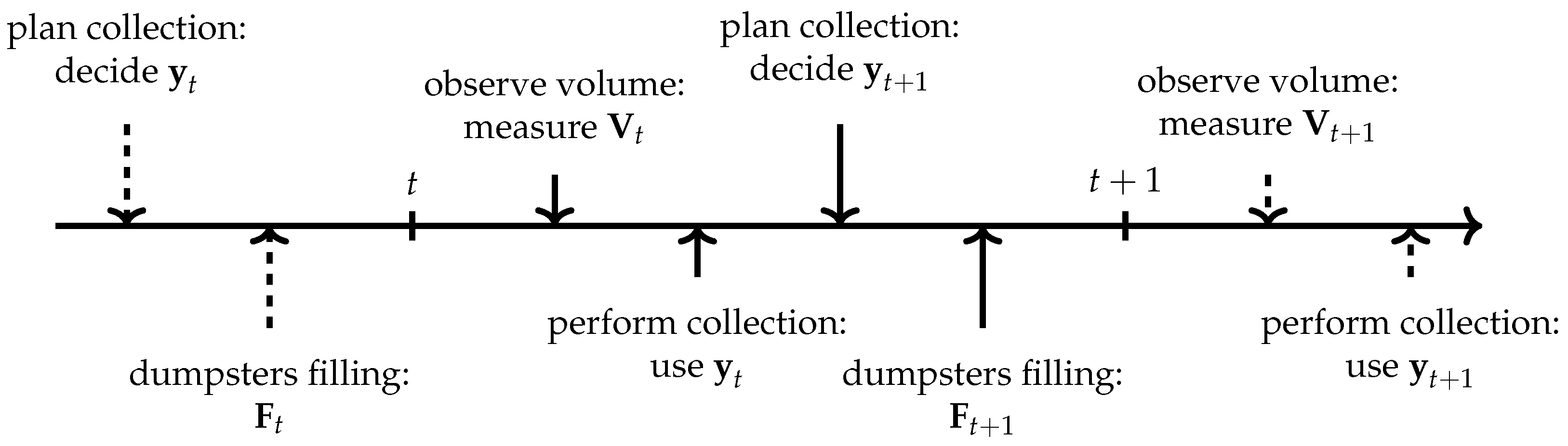
where $y_{i,t}$ is the binary decision variable equal to one if dumpster i is emptied at time t. As for $V_{i,t}$, we introduce the vectors ${\mathbf{F}}_t\doteq [F_{1,t},\dots ,F_{I,t}]$ and ${\mathbf{y}}_t\doteq [y_{1,t},\dots ,y_{I,t}]$. The system dynamic is summarized in Figure 1.

It is important to highlight that the collection for time step t is planned before we observe ${\widehat{\mathbf{V}}}_t$, since the measurements are either performed by the vehicle (during the collection at time t) or collected by the sensors that can make a measurement before the waste volume increment. These dynamics model the real decision-making process in which operational managers decide the collection plans at the end of their work day, and these decisions are implemented during the early morning of the day after (roughly 6–8 h later).

The physical state $V_{i,t}$ is measured by a noisy estimation, called ${\widehat{V}}_{i,t}$, defined as follows:

$${\widehat{V}}_{i,t}=V_{i,t}+{\epsilon }_i,{\epsilon }_i\sim \mathcal{N}(0,{}^m\sigma _i^2),$$

(2)

where ${}^m\sigma _i^2$ is the variance in the measurement error and can either be equal to ${}^{m\left(s\right)}\sigma _i^2$ if the measurement is performed by a sensor installed inside the dumpster or to ${}^{m\left(v\right)}\sigma _i^2$ if it is performed by the vehicle. We assume that ${}^{m\left(s\right)}\sigma _i^2<{}^{m\left(v\right)}\sigma _i^2$, since the volumetric sensors perform a direct measure. If a sensor is installed in the dumpster, then the measurements are made daily; otherwise, they are made during the vehicle’s collection. These measurements are used to create an up-to-date historical record of fillings and track the current waste volume. For the first scope, both sensor and vehicle measurements are used; for the second, only sensor ones are useful, since vehicle measurements are performed as the dumpster is emptied, and therefore the current waste volume is known to be zero. Using these observations, we build $V_{i,t}$, a distributional forecast, i.e., a distribution used to express the uncertainty in the physical state $V_{i,t}$ (see Section 4).

The main goal of this study is to find the subset of dumpsters in which to install the sensors, represented by a vector $\mathbf{z}\in {\{0,1\}}^I$ where each component $z_i$ is a binary variable equal to one if a sensor is installed inside dumpster i and zero otherwise. The information collected from the sensors and the vehicle is used to decide the subset of dumpsters to collect. This choice is modeled through the previously defined array ${\mathbf{y}}_t\in {\{0,1\}}^I$, whose elements are the binary variables $y_{i,t}$ equal to one if dumpster i is visited during time t. Given these decisions, the final routing is modeled by the matrix $X_t\in {\{0,1\}}^{\overline{I}\times \overline{I}}$, whose elements are the binary variables $x_{i,j,t}$ equal to one if the vehicle traverses the arc connecting node $i\in \overline{\mathcal{I}}$ to node $j\in \overline{\mathcal{I}}$, while $j\ne i$ during time step t. $X_t$ is constructed in such way that it respects the TSP’s subtour elimination constraints. Variables $x_{i,j,t}$ and $y_{i,t}$ are linked by the constraints

$$y_{i,t}=\sum _{j=1,j\ne i}^{\overline{I}}{x}_{i,j,t}\forall i\in \mathcal{I},$$

(3)

which enforce that variables $x_{i,j,t}$ are different from zero if the corresponding $y_{i,t}$ is set to one.

We provide an example to better understand the solution of each subproblem. We consider a simple instance with three dumpsters (denoted, in this example, by $d_1$, $d_2$, and $d_3$), in which $d_1$ and $d_2$ are relatively close to each other, to the depot (denoted by $d_O$), and to the dump (denoted by $d_D$), while $d_3$ is further away. Since the proximity among dumpsters discourages all of them being sensorized, we can reasonably expect that $d_3$, as well as one between $d_1$ and $d_2$—let us say $d_2$—will be equipped with a sensor. We therefore have $\mathbf{z}=[0,1,1]$. The collection and routing subproblems are solved for each time instant, and thus we focus on a single day $t^{\prime }$. We imagine that on day $t^{\prime }$, the sensor inside $d_3$ signals a low level of waste such that the algorithm considers its visit inconvenient. On the contrary, the measurements from dumpster $d_1$ and the waste estimate from dumpster $d_2$ signal a higher risk of overflow, making the short trip to them worthwhile. The algorithm therefore selects ${\mathbf{y}}_{{\mathbf{t}}^{\prime }}=[1,1,0]$. Lastly, the solver determines that it is optimal to visit $d_2$ before $d_1$ (since traveling the same path in opposite directions can result in different covered distances due to one-way roads or obstacles), ultimately setting

$$X_{t^{\prime }}=\begin{array}{c}\\ \hfill d_O\\ \hfill d_1\\ \hfill d_2\\ \hfill d_3\\ \hfill d_D\end{array}\begin{array}{ccccccc}& d_O& d_1\hfill & d_2& d_3& d_D& \\ (& \begin{array}{c}0\\ 0\\ 0\\ 0\\ 0\end{array}& \begin{array}{c}0\\ 0\\ 1\\ 0\\ 0\end{array}& \begin{array}{c}1\\ 0\\ 0\\ 0\\ 0\end{array}& \begin{array}{c}0\\ 0\\ 0\\ 0\\ 0\end{array}& \begin{array}{c}0\\ 1\\ 0\\ 0\\ 0\end{array}& )\end{array}$$

which represents the route $d_O\to d_2\to d_1\to d_D$.

According to [31], we compute the total solution cost as the sum of sensor installation and maintenance, routing, and collection costs. Since the action at time t affects the following decisions, and since the underlying system is stochastic, we aim to minimize the total expected cost; in other words, we have

$$\mathbb{E}[\sum _{t\in \mathcal{T}}\left(C_{sensors}\left(\mathbf{z}\right)+C_{collection}\left({\mathbf{y}}_t\right)+C_{routing}\left(X_t\right)\right)|{\mathbf{V}}_0],$$

(4)

where $C_{sensors}\left(\mathbf{z}\right)$ is the cost of the sensors’ maintenance, $C_{collection}\left({\mathbf{y}}_t\right)$ is the overflow penalty cost, $C_{routing}\left(X_t\right)$ is the routing cost, and ${\mathbf{V}}_0$ is the state of the system at time step 0.

The cost required for the sensors’ maintenance is

$$C_{sensors}\left(\mathbf{z}\right)=\sum _{i=1}^I{\lambda }_i^M·z_i,$$

(5)

where the parameter ${\lambda }_i^M$ represents the expected daily maintenance cost (i.e., sensor’s connection, physical maintenance, cost for IT maintenance, etc.) of a single sensor together with its depreciation installment.

The collection cost accounts for the overflow penalty. In the formula

$$C_{collection}\left({\mathbf{y}}_t\right)=\sum _{i=1}^I{\lambda }_i^O·max(V_{i,t}·(1-y_{i,t})-Q_i,0),$$

(6)

where the parameter ${\lambda }_i^O$ represents the cost per unit of overflowing waste volume in dumpster i, it is important to notice that when collection of a dumpster is performed at a specific time step ($y_{i,t}=1$), even if the waste volume briefly overcomes the dumpster’s capacity on the same day ($V_{i,t}>Q_i$), no overflow penalty is imposed.

Finally, the routing cost is defined by

$$C_{routing}\left(X_t\right)=\sum _{(i,j)\in \mathcal{A}}{c}_{i,j}·x_{i,j,t}$$

(7)

where the parameter $c_{i,j}$ expresses the cost of traversing the arc connecting node i to node j.

We summarize the model variables and parameters in

Table 2. Variables and parameters of the mathematical model. Stochastic elements are marked by ⋆.

Variable		Description
$z_i\in \{0,1\}$		Set to 1 if dumpster i is equipped with a sensor, 0 otherwise
$y_{i,t}\in \{0,1\}$		Set to 1 if dumpster i is collected at day t, 0 otherwise
$x_{i,j,t}\in \{0,1\}$		Set to 1 if the route $i-j$ is traversed by the vehicle at day t, 0 otherwise
Parameter		Description
I		Number of dumpsters
T		Number of simulated days used for solution evaluation
S		Number of scenarios
$Q_i$		Capacity of vehicle i
$V_{i,t}$	⋆	Waste volume for dumpster i at day t
${\widehat{V}}_{i,t}$		Measurement of waste volume for dumpster i at day t
${\tilde{V}}_{i,t}$	⋆	Estimate of waste volume for dumpster i at day t
$F_{i,t}$	⋆	Waste volume increment of dumpster i at day t
${\tilde{F}}_{i,t}$	⋆	Estimate of waste volume increment of dumpster i at day t
${\tilde{V}}_{i,t}^s$	⋆	Estimate of waste volume for dumpster i at day t in scenario s
${\lambda }^R$		Routing cost coefficient
${\lambda }^O$		Penalty cost associated with dumpster overflow
${\lambda }^M$		Sensor installation and maintenance cost

.

4. Solution Heuristics

In this section, we present the adopted solution method. In Section 4.1, we focus on the collection plan problem, i.e., finding the optimal set of dumpsters to be visited by the vehicle for each time step and their optimal order of visiting. Then, in Section 4.2, we present the methodology developed for solving the sensor placement subproblem. We do not address the routing problem in detail, since we solve it using a commercially available TSP solver. However, it is important to highlight that our modular approach allows for alternative methods to compute both the duration and length of the tour. This flexibility opens the door not only to other optimization techniques, but also—perhaps more interestingly—to estimation methods tailored to assessing driver performance. For example, the routing component can be adapted to incorporate driver-specific knowledge that may not be captured by general-purpose online services like Google Maps. For example, drivers may know where cars are typically parked in ways that block the passage of the vehicle, or they may be aware of school entrance times (thus avoiding certain streets or dumpsters during peak hours due to the traffic caused by parents dropping off their children). Moreover, drivers may have individual preferences based on their skill and familiarity with the area; some may prefer narrow streets to minimize travel distance, while others may opt for wider roads that allow for faster driving. Such flexibility highlights the practicality and adaptability of our method in real-world scenarios.

4.1. Collection Plan

Given a sensor placement $\mathbf{z}$, we decide the optimal set of dumpsters to be visited by considering Equation (4). Since optimizing Equation (4) requires solving a complex multistage stochastic optimization problem, we estimate the expected value in Equation (4) by using the volume measurements gathered in the previous time steps, and instead of computing the sum over all the future time steps, we use a one-step look-ahead strategy. In the formula, we minimize

$${\displaystyle \frac{1}{\left|\mathcal{S}\right|}}\sum _{s\in \mathcal{S}}\left[\sum _{i=1}^I{\lambda }_i^{O}max({\tilde{V}}_{i,t}^s·(1-y_{i,t})-Q_i,0)\right]+\sum _{(i,j)\in \mathcal{A}}{c}_{i,j}·x_{i,j,t},$$

(8)

where $\mathcal{S}$ is a set of equiprobable scenarios and ${\tilde{V}}_{i,t}^s$ is an estimate of the volume realization in scenario s. Note that in Equation (8), we do not consider the term related to sensor installation as it is a constant for a fixed $\mathbf{z}$. To define the scenario realizations ${\tilde{V}}_{i,t}^s$, we need to study the uncertainty affecting $V_{i,t}$, which is composed of two different stochastic contributions. The first arises from the fact that we are making a decision at time t, but we have no way of gathering information about the waste volume of the dumpsters past time $t-1$. (At best, $V_{i,t-1}$ can potentially be estimated through a direct sensor measurement ${\widehat{V}}_{i,t-1}$, or it can be known to be equal to zero if at time $t-1$, the vehicle collected its contents.) Between times $t-1$ and t, one filling event invariably takes place, and therefore this contribution is always present and irreducible. The second depends on whether the last information on the waste volume of the dumpster is indeed gathered at time $t-1$ or even earlier. If a sensor is used, then we are sure to have a measurement at time $t-1$; otherwise, unless the waste was collected at time $t-1$, the last direct information comes from collections at previous time instants, introducing more filling events for which we have no data (however, we know that the waste volume right after collection was zero). We call ${\Delta }_{i,t}$ the number of time steps which elapsed from the last collection performed on dumpster i to the current time instant t. Therefore, the estimate of the volume realization is computed as follows:

• If collection was performed at time $t-1$,

  $${\tilde{V}}_{i,t}={\tilde{F}}_{i,t}\forall i\in \mathcal{I}.$$

  (9)
• Otherwise, if dumpster i is equipped with a sensor,

  $${\tilde{V}}_{i,t}={\widehat{V}}_{i,t-1}+{\tilde{F}}_{i,t}\forall i\in \mathcal{I}.$$

  (10)
• Otherwise,

  $${\tilde{V}}_{i,t}=\sum _{t^{\prime }=t-{\Delta }_{i,t}}^t{\tilde{F}}_{i,t^{\prime }}\forall i\in \mathcal{I}.$$

  (11)

${\tilde{F}}_{i,t}$ is the distributional forecast of the random waste volume increment in the dumpster, and using a data-driven approach, we assume that for any t, the distribution of ${\tilde{F}}_{i,t}$ is a discrete uniform one where each value is a historical filling estimation. In other words, we are considering that the possible realizations of each of the fillings are identical to one of those that has already been realized in the past. We call $m_i$ the number of historical filling estimations for dumpster i. Each combination of fillings characterizes a scenario s.

If a sensor is installed in the dumpster, then the number of scenarios is equal to $m_i$. Contrarily, without the sensor, the number of scenarios is equal to $({\displaystyle \genfrac{}{}{0pt}{}{m_i+{\Delta }_{i,t}-1}{{\Delta }_{i,t}}})$, since each of the ${\Delta }_{i,t}$ considered filling events (${\Delta }_{i,t}>=1$) can consist of one of $m_i$ possible volume values. For this reason, a subset of $m_i·{\Delta }_{i,t}$ is instead sampled and used in Equation (8). When ${\Delta }_{i,t}=1$ (the dumpster was collected at time $t-1$), it is easy to see that $({\displaystyle \genfrac{}{}{0pt}{}{m_i+{\Delta }_{i,t}-1}{{\Delta }_{i,t}}})=m_i·{\Delta }_{i,t}=m_i$, and thus all scenarios are used similar to when a sensor is present.

We therefore draw samples of the realizations independently one from the other yet all with the same probability. In doing so, we are neglecting seasonality, but this is not a strong assumption since it could theoretically be circumvented by adopting more complex probability distributions.

To find the values of ${\mathbf{y}}_t$ and $X_t$ which minimize Equation (8), it is enough to focus on ${\mathbf{y}}_t$, since $X_t$ is always consequently computed by a routing solver. We compute ${\mathbf{y}}_t$ using an iterative procedure that starts from $y_{i,t}=0$, where $\forall i\in \mathcal{I}$. Then, an iterative loop modifies the current solution in the following way:

• For each dumpster not in the current solution, we compute the cost of the current solution with that dumpster added. If the cost is lower than the one for the current solution, then we put it in the list of dumpsters to add.
• For each dumpster in the current solution, we compute the cost of the current solution with that dumpster removed. If the cost is lower than the one for the current solution, then we put it in the list of dumpsters to remove.
• We add to the current solution all the dumpsters in the first list, remove the ones in the second one, and then repeat the procedure from the first step. If no dumpster is added or removed, or if the newly obtained solution was already obtained, then we break the loop to avoid looping forever.

The procedure is summarized in Algorithm 1.

Algorithm 1 Daily collection scheduling algorithm.

1:  ${\mathbf{y}}_t^{new}=\mathbf{0}$   2:  ${\mathbf{y}}_t=\mathtt{None}$   3:  $\mathtt{previous}\_\mathtt{solutions}=\left[\right]$   4:  while ${\mathbf{y}}_t^{new}\ne {\mathbf{y}}_t \& {\mathbf{y}}_t$ not in $\mathtt{previous}\_\mathtt{solutions}$ do   5:        ${\mathbf{y}}_t={\mathbf{y}}_t^{new}$   6:        $\mathtt{to}\_\mathtt{add}=\left[\right]$   7:        $\mathtt{to}\_\mathtt{remove}=\left[\right]$   8:        for $y_{i,t}$ in ${\mathbf{y}}_t$ do   9:              ${\mathbf{y}}_t^{\prime }={\mathbf{y}}_t$ 10:              if $y_{i,t}=0$ then 11:                    $y_{i,t}^{\prime }=1$ 12:                    if $C\left({\mathbf{y}}_t^{\prime }\right)<C\left({\mathbf{y}}_t\right)$ then 13:                          $\mathtt{to}\_\mathtt{add}.\mathtt{append}($i) 14:                    end if 15:              end if 16:              if $y_{i,t}=1$ then 17:                    $y_{i,t}^{\prime }=0$ 18:                    if $C\left({\mathbf{y}}_t^{\prime }\right)<C\left({\mathbf{y}}_t\right)$ then 19:                          $\mathtt{to}\_\mathtt{remove}.\mathtt{append}($i) 20:                    end if 21:              end if 22:        end for 23:        for i in $\mathtt{to}\_\mathtt{add}$ do 24:              $y_{i,t}^{new}=1$ 25:        end for 26:        for i in $\mathtt{to}\_\mathtt{remove}$ do 27:              $y_{i,t}^{new}=0$ 28:        end for 29:        $\mathtt{previous}\_\mathtt{solutions}.\mathtt{append}\left({\mathbf{y}}_t^{new}\right)$ 30:  end while

The complexity of the algorithm for the collection plan is $\mathcal{O}(\gamma ·I·\mathrm{TSP}(I\left)\right)$, where I is the number of dumpsters and $\gamma$ is the number of local search iterations until convergence. $\mathrm{TSP}\left(I\right)$ represents the complexity of the TSP algorithm with respect to the number of nodes. The solver we used for the numerical experiments was OR Tools (https://developers.google.com/optimization/routing/, accessed on 5 January 2026), for which no precise Big-O characterization exists.

4.2. Sensor Placement

The sensor placement problem was tackled via ALNS, which employs a set of operators to iteratively modify the current solution $\mathbf{z}$ and obtain a neighboring one ${\mathbf{z}}^{\prime }$. The operators were split into destroy (${\mathsf{O}}_k^d$, $k\in \mathcal{K}=\{1,\dots ,K\}$) and repair (${\mathsf{O}}_l^r$, $l\in \mathcal{L}=\{1,\dots ,L\}$). The former removed sensors from $\mathbf{z}$ while the latter added them. At each iteration, ${\mathbf{z}}^{\prime }={\mathsf{O}}_l^r\left({\mathsf{O}}_k^d\left(\mathbf{z}\right)\right)$ was obtained. We considered three destroy and three repair operators:

• ${\mathsf{O}}_1^d$ and ${\mathsf{O}}_1^r$ are the identity operators, which did not alter the solution.
• ${\mathsf{O}}_2^d$ (${\mathsf{O}}_2^r$) removed (added) a random sensor from (to) the solution with a uniform distribution.
• ${\mathsf{O}}_3^d$ (${\mathsf{O}}_3^r$) removed (added) a sensor from (to) the solution. The sensor was chosen randomly with a probability inversely proportional to the sum of distances to all other sensors currently in (not in) the solution. The rationale was to distribute the sensors far from each other.

While ${\mathsf{O}}_1^d$, ${\mathsf{O}}_1^r$, ${\mathsf{O}}_2^d$, and ${\mathsf{O}}_2^r$ are operators commonly used in ALNS, ${\mathsf{O}}_3^d$ and ${\mathsf{O}}_3^r$ represent an added value of our study since they are not usual in this context.

The operator selection was performed in such a way that one destroy operator was chosen randomly from the set of all destroy operators at every iteration. Each destroy operator had a probability $p_k^d$ of being selected. The same was true for the repair operators, where the probabilities were $p_l^r$. Some adjustments were made to make sure it was impossible for the algorithm to select ${\mathsf{O}}_1^d$ and ${\mathsf{O}}_1^r$ simultaneously so as to avoid ${\mathbf{z}}^{\prime }=\mathbf{z}$.

The probabilities $p_k^d$ ($p_l^r$) were computed as follows:

$$p_k^d={\displaystyle \frac{q_k^d}{{\sum }_{h=1}^K{q}_h^d}}\left(p_l^r={\displaystyle \frac{q_l^r}{{\sum }_{h=1}^L{q}_h^r}}\right),$$

(12)

where $q_k^d$ ($q_l^r$) is the performance score of operator ${\mathsf{O}}_k^d$ (${\mathsf{O}}_l^r$) that quantifies its goodness based on the quality of the solutions found thus far. At each iteration of the ALNS, $q_k^d$ ($q_l^r$) was updated as follows:

$$q_k^d=q_k^d+\delta (q_l^r=q_l^r+\delta ),$$

(13)

where $\delta >0$ depends on the quality of ${\mathbf{z}}^{\prime }$.

To measure the quality of a solution, we ran a T-step simulation on a fixed scenario, obtaining

$$c\left(\mathbf{z}\right)=C_{sensors}\left(\mathbf{z}\right)+{\displaystyle \frac{1}{T}}\left\{\sum _{t=1}^T\left[C_{routing}\left(X_t\right)+C_{collection}\left({\mathbf{y}}_t\right)\right]\right\},$$

(14)

where $C_{routing}\left(X_t\right)$, $C_{collection}\left({\mathbf{y}}_t\right)$, and $C_{sensors}\left(\mathbf{z}\right)$ are described in Equations (5), (6), and (7), respectively. At each step of the simulation, $X_t$ and ${\mathbf{y}}_t$ were computed as described in Section 4.1.

It is worth noting that Equation (14) was averaged over time, since we aimed at obtaining the minimum average cost. We averaged over time instead of averaging over different scenarios, since the process is ergodic [35].

In Equation (14), $C_{sensors}\left(\mathbf{z}\right)$ depends directly on $\mathbf{z}$ and increases as more sensors are installed. Moreover, $\mathbf{z}$ also affects ${\mathbf{y}}_t$ through the information retrieved by the sensors, thus influencing $X_t$ and their associated costs $C_{collection}\left({\mathbf{y}}_t\right)$ and $C_{routing}\left(X_t\right)$. In general, the more sensors, the smaller both $C_{collection}\left({\mathbf{y}}_t\right)$ and $C_{routing}\left(X_t\right)$ become. Therefore, good solutions are characterized by a suitable trade-off between all the costs.

Whether the neighbor solution obtained through the operators is accepted as the new current solution depends on a solution acceptance policy. The solution acceptance policy is created through simulated annealing (SA), a metaheuristic method that allows non-improving solutions to be accepted with a certain probability, thus granting the algorithm the ability to escape local optima during exploration. In particular, given the current solution $\mathbf{z}$, the neighboring one ${\mathbf{z}}^{\prime }$ found by applying the ALNS operators, and the best solution found thus far ${\mathbf{z}}^{best}$, the SA acts as follows:

• If $c\left({\mathbf{z}}^{\prime }\right)<c\left({\mathbf{z}}^{best}\right)\le c\left(\mathbf{z}\right)$, then a new best solution is found, both $\mathbf{z}$ and ${\mathbf{z}}^{best}$ are set to ${\mathbf{z}}^{\prime }$, and the performance scores of the operators are increased by the amount $\delta ={\delta }_1$.
• If $c\left({\mathbf{z}}^{best}\right)<c\left({\mathbf{z}}^{\prime }\right)<c\left(\mathbf{z}\right)$, then $\mathbf{z}$ is set to ${\mathbf{z}}^{\prime }$, and $\delta ={\delta }_2<{\delta }_1$.
• Finally, if $c\left({\mathbf{z}}^{best}\right)\le c\left(\mathbf{z}\right)<c\left({\mathbf{z}}^{\prime }\right)$, then we set $\mathbf{z}$ to ${\mathbf{z}}^{\prime }$, and $\delta ={\delta }_3<{\delta }_2$ with a probability equal to

  $$exp\left(-{\displaystyle \frac{\Delta c}{\tau }}\right),$$

  (15)

  where $\Delta c=c\left({\mathbf{z}}^{\prime }\right)-c\left(\mathbf{z}\right)$. Otherwise, $\mathbf{z}$ is not updated, and $\delta =0$.

The parameter $\tau$ in Equation (15) is called the temperature. For large values of $\tau$, the probability of accepting non-improving solutions is high, while for small values of $\tau$, it is low. When the algorithm starts, $\tau$ is set to a value which leads Equation (15) to be close to one. Then, at each iteration of the algorithm, it is decreased. The decrement rule aims at constantly reducing the probability of acceptance by a factor of $\alpha$ every $\beta$ iterations; in other words, we have

$$exp\left(-{\displaystyle \frac{\Delta c^{(\kappa +1)}}{{\tau }^{(\kappa +1)}}}\right)={\displaystyle \frac{1}{\sqrt[\beta ]{\alpha }}}·exp\left(-{\displaystyle \frac{\Delta c^{\left(\kappa \right)}}{{\tau }^{\left(\kappa \right)}}}\right).$$

(16)

By replacing $\Delta c^{(\kappa +1)}$ and $\Delta c^{\left(\kappa \right)}$ with the average variation $\overline{\Delta c}$, we compute the decrementing rule as follows:

$${\tau }^{(\kappa +1)}={\displaystyle \frac{\overline{\Delta c}·{\tau }^{\left(\kappa \right)}}{\overline{\Delta c}+\frac{ln\alpha }{\beta }·{\tau }^{\left(\kappa \right)}}}.$$

(17)

Finally, if U consecutive neighbor solutions were not accepted, then we reset the temperature to the initial value, and when R resets were completed, we stopped the algorithm.

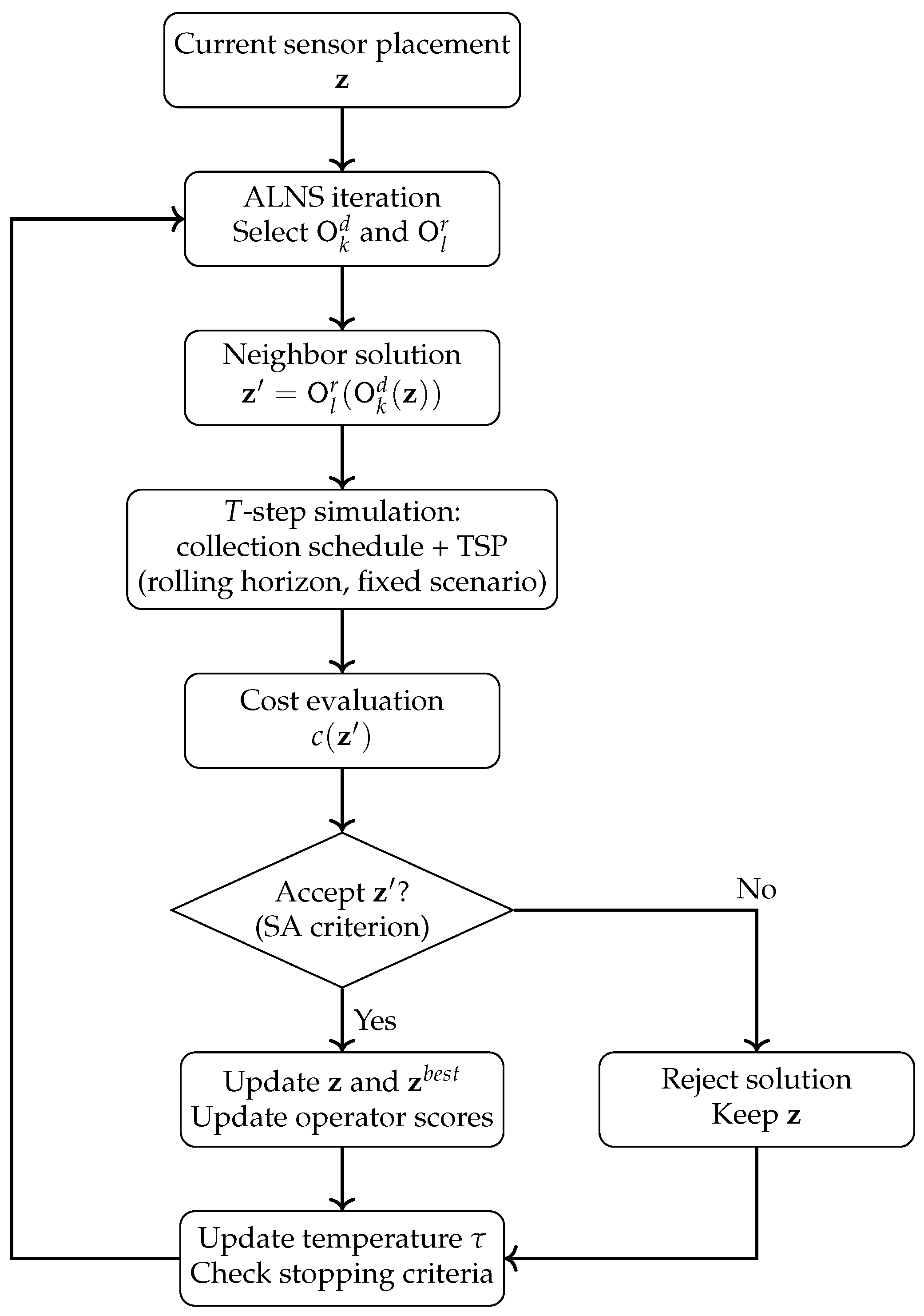
It is worth mentioning that we performed a preliminary study on different approaches to tackle the sensor placement problem, in which we also tested variable neighborhood search and large neighborhood search. Nevertheless, the best performances, which are presented in the following section, were obtained using the described ALNS. The implementations and results of the other heuristics were omitted from this study both for the sake of brevity and because they were irrelevant with respect to the aim of the paper. We report in Figure 2 the flowchart of the algorithm.

The complexity of the algorithm for the collection plan is $\mathcal{O}(\gamma ·R·U·T·I·\mathrm{TSP}(I\left)\right)$, where I is the number of dumpsters, T is the number of simulated days, U and R are the temperature reset parameters introduced in this section, $\gamma$ is the number of local search iterations until convergence, and $\mathrm{TSP}\left(I\right)$ is the complexity of the TSP algorithm with respect to the number of nodes. It is worth noting that in practice, U, R, and $\gamma$ are limited, and the algorithm runs in a reasonable time for real-world instances.

5. Numerical Experiments

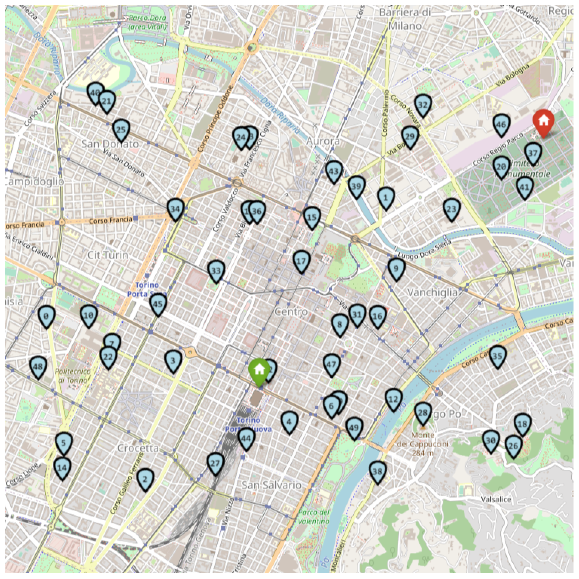
In this section, we evaluate the performance of the algorithm in realistic instances for the city of Torino. We consider 50 dumpsters which belonged to the same district and were therefore grouped together and assigned for collection to a single vehicle. We show the map of these in Figure 3. The first instance used cost parameters extracted from real data and evaluated the performance of the proposed algorithm. Then, two benchmark instances used the same parameters but equipped none and all of the dumpsters with sensors. Lastly, in Section Sensitivity Analysis, 12 further instances help us to perform sensitivity analysis with respect to the cost parameters and the standard deviation of sensor measurement errors.

Each time step t represents a collection day. We solved the routing problem using OR Tools v9.12, a freely available constraint programming solver provided by Google.

We considered each arc cost $c_{i,j}$ to be directly proportional to the time spent by the vehicle moving across the same arc; in other words, we have

$$c_{i,j}={\lambda }_{i,j}^R·t_{i,j},$$

(18)

where ${\lambda }_{i,j}^R$ is the cost per time unit spent on the road between nodes i and j for collection. According to real data provided by Cidiu S.p.A. (https://cidiu.it/, accessed on 5 January 2026), we set ${\lambda }_{i,j}^R=0.25$ €/s, the expected daily maintenance cost ${\lambda }_i^M=10$ €/sensor, and the cost per unit of overflowing waste volume ${\lambda }_i^O=10$ €/L. Since ${\lambda }_{i,j}^R$, ${\lambda }_i^M$, and ${\lambda }_i^O$ are constant and do not depend on the single dumpster, in the following, we will remove their subscripts.

We sampled the fillings of the dumpsters from a normal distribution $\mathcal{N}({}^f\mu _i,{}^f\sigma _i^2)$, where both the mean ${}^f\mu _i$ and the standard deviation ${}^f\sigma _i$ were estimated from the data of Cidiu S.p.A. This ensured that the model was realistic, even taking into account the difference in the data for dumpsters that were close together. The standard deviation of the measurement error was instead set to ${}^{m\left(v\right)}\sigma _i=0.10·Q_i$ (vehicle measurements) and ${}^{m\left(s\right)}\sigma _i=0.05·Q_i$ (sensor measurements). In this way, regardless of the considered dumpster, the ratio ${\displaystyle \frac{{}^{m\left(s\right)}\sigma _i}{{}^{m\left(v\right)}\sigma _i}}$ was equal to $0.5$.

To ensure a reasonable starting condition for the system and a sufficient amount of data to be fed to the algorithm, we employed a starting set of 14 volumetric measures for each dumpster, and we used it to perform 14 preliminary days of collection (without any sensors). Then, we decided the positions of the sensors (using the algorithm described in Section 4.2), and we set $T=60$ in Equation (14) to evaluate the solution. Finally, we tested the solution obtained in a rolling horizon fashion for 360 days.

Concerning the ALNS, we set ${\delta }_1=0.5$, ${\delta }_2=0.3$, and ${\delta }_3=0.1$. Moreover, for the SA, the best value of R was obtained empirically; while the computational time increased approximately linearly with R, the most significant improvements to the solution were always observed well before the fifth temperature reset, and thus $R=5$ was set. Based on a similar empirical campaign, we set $\alpha =2$ and $\beta =5$.

Since U controls the stopping condition for the exploration, we set it with a mathematical approach. Let us denote by $\pi$ the improvement ratio of solutions in the neighborhood. When we approached the optimal solution and $\pi$ decreased, so did the probability of picking one of those improving solutions. For a reference value of $\pi$, we chose the value of U such that there was a $50\%$ probability of finding one of those improving solutions:

$$1-{(1-\pi )}^U=50\%\Rightarrow U={\displaystyle \frac{log(50\%)}{log(1-\pi )}}.$$

(19)

A good compromise between computational time and performance was obtained by considering $\pi =3.4\%$ so that $U=20$. In other words, the chance of improving the solution was kept above 50% as long as the ratio of improving solutions in the neighborhood was above 3.4%.

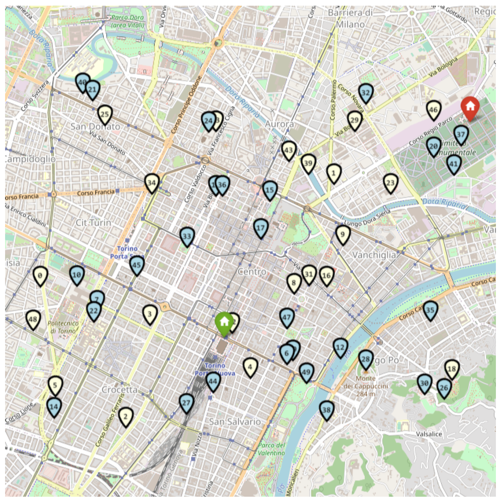
Using the parameters and the instance described above, the resulting set of sensorized dumpsters is shown in Figure 4, and it consists of 21 sensors. We compared three configurations over a 360-step-long period: no sensors (referred to as 0 sensors), representing the current solid waste collection operation; all sensors installed (50 sensors); and the recommended subset (21 sensors). The results are reported in

Table 3. Cost comparison among different sensor configurations.

	0 Sensors	21 Sensors	50 Sensors
Routing cost	636,944.90 €	538,467.80 €	426,017.65 €
Collection cost	977.08 €	6688.71 €	29,269.79 €
Sensor cost	0.00 €	75,600.00 €	180,000.00 €
Total cost	637,921.98 €	620,756.51 €	635,287.44 €

.

The use of volumetric sensors proved itself to be useful for reducing the overall waste collection process costs; according to the simulation, approximately 17,000 € could be saved yearly by strategically installing sensors in a portion of the dumpsters. The optimal solution from an economic point of view also achieves the sustainability objective of lowering the environmental impact of the operations by reducing the emissions by 15.5%. It is worth noting that the scenario with 21 sensors performed better than that with 50 sensors, proving that the cost for sensor maintenance can be more than the value of the information that it collects.

If we compare the scenarios with 21 sensors to 0 sensors, we notice that in the former, the sum of the annual collection and routing costs was lower by 92,765.47 €, while the annual maintenance costs of the sensors were higher by 75,600.00 €. This suggests that, on average, each of the 21 sensors could save approximately 4417.40 € in collection and overflow costs while only requiring 3600.00 € for maintenance. Instead, if we compare the scenario with 50 sensors against that with 21 sensors, the average savings of the additional 29 sensors was 3098.93 € each, which is lower than their maintenance cost if installed. This empirically proves that the relative worth of the sensors depends on their location.

We also notice that the collection cost increased with the number of installed sensors. While counterintuitive, this result derives from the algorithm being able to make precise choices when presented with reliable and frequent information from the sensors, resulting in more frequent low-volume overflows. On the other hand, when faced with scarcer information—when no sensors were installed in the dumpsters—the algorithm was quite conservative with respect to the possibility of high-volume overflows occurring. Additional information therefore allows the algorithm to strategically plan economically convenient waste overflows. Ultimately, the choice between more frequent collection and possible overflows is determined by the importance (economical or social) that is given to both. However, since giving an economical impact to a social issue is often difficult, in the following, we include a study on what happens when we consider different overflow penalty costs.

Sensitivity Analysis

In this section, we test the results obtained in the previous one by perturbing the costs ${\lambda }^O$, ${\lambda }^M$, and ${\lambda }^R$.

If the overflow penalty cost coefficient decreased to ${\lambda }^O=5$ €/L, then the number of sensors installed decreased to 20. This solution achieved a total cost of 611,446.19 €, which is lower than the previous one. Nevertheless, this decrease was due to the algorithm taking advantage of allowing overflows since the penalty was low. This was also confirmed in the extreme case ${\lambda }^O=0$ €/L, where the total cost was null as there was no collection, and all dumpsters were overflowing each day.

If ${\lambda }^O$ were instead increased to ${\lambda }^O=15$ €/L, then the total costs would amount to 642,570.26 €. This increase in the overflow penalty cost coefficient can potentially reflect a will to avoid overflows as much as possible, accounting for an additional social value.

In short, on the one hand, a low penalty cost allows too many overflows, but on the other, a high one can potentially incentivize the algorithm to be too conservative and aggressively visit the majority of the dumpsters each day.

Table 4. Characteristics of the proposed solution for different overflow penalty cost coefficients.

${\mathit{\lambda }}^{\mathit{O}}$	5 €/L	10 €/L	15 €/L
No. of sensors	20	21	7
Total cost	611,446.19 €	620,756.51 €	642,570.26 €
Routing cost	532,114.73 €	538,467.80 €	616,030.42 €
Collection cost	7331.47 €	6688.71 €	1339.83 €
Sensor cost	72,000.00 €	75,600.00 €	25,200.00 €
Emissions	22,640 kg CO2	22,911 kg CO2	26,201 kg CO2
Overflow	1466 L	669 L	89 L

shows the results, which include CO₂ emissions, calculated using an average emission value (https://www.ecocerved.it/media/2010-08-30_trasporto, accessed on 5 January 2026) of 765 g CO₂/km and considering an average speed of 50 km/h, as per urban area regulations.

Concerning the cost per time unit spent on the road ${\lambda }^R$, we considered it to vary in the set $\{0.20,0.24,0.25,0.26,0.30\}$ €/s, where ${\lambda }^R=0.25$ €/s is the value used in the previous section. We report the results in

Table 5. Results for different costs per time unit traveled during collection.

${\mathit{\lambda }}^{\mathit{R}}$	0.20 €/s	0.24 €/s	0.25 €/s	0.26 €/s	0.30 €/s
No. of sensors	2	18	21	22	41
Total cost	514,202.00 €	605,914.97 €	620,756.51 €	667,808.23 €	715,182.74 €
Routing cost	505,140.10 €	539,485.56 €	538,467.80 €	557,905.30 €	537,064.95 €
Collection cost	1861.90 €	1629.41 €	6688.71 €	30,702.93 €	30,517.79 €
Sensor cost	7200.00 €	64,800.00 €	75,600.00 €	79,200.00 €	147 600.00 €
Emissions	26,851 kg CO2	23,906 kg CO2	22,911 kg CO2	22,797 kg CO2	19,048 kg CO2
Overflow	187 L	163 L	669 L	3071 L	3052 L

.

It is possible to notice that the total annual emissions were lower the higher ${\lambda }^R$ became. Moreover, the total annual cost increased as ${\lambda }^R$ increased, while the annual routing cost remained almost the same. On the one hand, more overflows were allowed to happen as they became less expensive than the collection. On the other, and more prominently, the installation of a higher number of sensors enabled better collection decisions.

We varied the expected daily maintenance cost ${\lambda }^M$ in the set $\{7.5,9,10,11,12.5\}$ €/day, with ${\lambda }^M=10$ €/day being the value used in the previous section. The results are shown in

Table 6. Results for different daily sensor maintenance costs.

${\mathit{\lambda }}^{\mathit{M}}$	7.5 €/Day	9 €/Day	10 €/Day	11 €/Day	12.5 €/Day
No. of sensors	46	21	21	15	3
Total cost	591,509.90 €	613,196.51 €	620,756.51 €	637,720.66 €	641,586.67 €
Routing cost	436,981.25 €	538,467.80 €	538,467.80 €	562,920.97 €	624,957.55 €
Collection cost	30,328.65 €	6688.71 €	6688.71 €	15,399.69 €	3129.12 €
Sensor cost	124,200.00 €	68,040.00 €	75,600.00 €	59,400.00 €	13,500.00 €
Emissions	18,589 kg CO2	22,911 kg CO2	22,911 kg CO2	23,944 kg CO2	26,583 kg CO2
Overflow	3033 L	669 L	669 L	1540 L	313 L

.

When ${\lambda }^M$ increased, the total annual cost increased (as for ${\lambda }^R$), while the sensor cost decreased since the solution provided by the algorithm installed fewer sensors.

While the parameter ${\lambda }^O$ regulated the amount of waste overflow but had a small influence on the number of sensors installed, both ${\lambda }^R$ and ${\lambda }^M$ had a much bigger impact on it.

In both the analysis of ${\lambda }^R$ and ${\lambda }^M$, it is possible to notice that when a higher number of sensors was employed, the collection cost increased in favor of lowering the routing cost, thus reaching an equilibrium dictated by the relationship between ${\lambda }^R$ and ${\lambda }^O$.

Finally, we considered ${}^{m\left(s\right)}\sigma _i$ to vary in the set $\{0.05·Q_i,0.075·Q_i,0.1·Q_i\}$, resulting in the following ratios between the standard deviation of the error from the sensors and the one from the vehicle: ${\displaystyle \frac{{}^{m\left(s\right)}\sigma _i}{{}^{m\left(v\right)}\sigma _i}}\in \{0.5,0.75,1\}$.

Table 7. Results for different standard deviations of sensor measurement errors.

	${}^{\mathit{m}\left(\mathit{s}\right)}\mathit{\sigma }_{\mathit{i}}=0.05·{\mathit{Q}}_{\mathit{i}}$	${}^{\mathit{m}\left(\mathit{s}\right)}\mathit{\sigma }_{\mathit{i}}=0.075·{\mathit{Q}}_{\mathit{i}}$	${}^{\mathit{m}\left(\mathit{s}\right)}\mathit{\sigma }_{\mathit{i}}=0.1·{\mathit{Q}}_{\mathit{i}}$
No. of sensors	21	14	0
Total cost	620,756.51 €	633,444.67 €	637,921.98 €
Routing cost	538,467.80 €	577,116.40 €	636,944.90 €
Collection cost	6688.71 €	5928.27 €	977.08 €
Sensor cost	75,600.00 €	50,400.00 €	0 €
Emissions	22,911 kg CO2	24,556 kg CO2	27,081 kg CO2
Overflow	669 L	593 L	98 L

shows the results for these three cases.

The total cost increased slightly as the error’s standard deviation increased, resulting in saving approximately 17,000 € in the first case and 4500 € in the second one with respect to the zero-sensor solution. Moreover, the total emissions were lower by 15.5% and 9.4%, respectively, which is crucial when evaluating not only the economic impact but also the environmental impact of the solution.

While in the third case the best configuration consisted of not installing any sensors, we were able to find other interesting suboptimal solutions. In particular, one suggested the installation of 21 sensors and achieved a total cost of 638,590.38 € (subdivided into 560,831.75 € for routing, 2158.63 € for collection, and 75,600.00 € for sensors) with the total emissions amounting to 23,868 kg CO₂ and a total overflow of 216 L. By accepting a total cost increase of approximately 600 €, the routing cost—and emissions—could be reduced by 12.0% even if ${}^{m\left(s\right)}\sigma _i={}^{m\left(v\right)}\sigma _i$, proving that the value of the sensors is not only in the quality of the measurements but also in providing more data.

These last considerations link back to the sensitivity analysis of ${\lambda }^R$ (the cost per time unit spent on the road), with the additional possible future development of adapting this parameter to also model the environmental impact of the sector from an ethical point of view.

6. Conclusions

This study focused on the problem of deciding the optimal location for volumetric sensors as well as quantifying the value coming from the information that they collect. The main contribution of this study therefore lies in simultaneously addressing both the collection planning and the sensor placement problems, with the added asset of volumetric sensors installed directly on the vehicle. To the best of our knowledge, modeling and tackling the interdependence between the two problems constitutes a novelty in the field of solid waste collection.

To decide the positions of the sensors, we used heuristics based on adaptive large neighborhood search. We tested it over a realistic instance of 50 dumpsters in the city of Torino. The results show that equipping 21 selected dumpsters with sensors can save up to 17,000 € yearly while also reducing emissions by 15.5%.

We investigated how these results varied with respect to the parameters of the problem through a sensitivity analysis, showing that the optimal number of sensors to employ and the related economic advantages closely depend on the characteristics of the instance. For example, when the cost per time unit traveled during collection grew and the vehicle movement became more costly, the number of installed sensors increased. On the contrary, when the sensor cost was large, few sensors were installed, and the emissions increased as a consequence of poorer information. Finally, we show the benefits of the installation of sensors even when their measurements’ uncertainty was equal to the vehicle’s. In this setting, no cost saving was achieved with respect to not employing any sensor. Nonetheless, the total emissions were reduced by 12%. This highlights how the value of sensors resides not only in the measurements’ quality but also in their quantity.

An obvious limitation of this study is the restriction imposed by how municipality waste collection is currently managed by the city of Torino, where the dumpsters are divided into clusters, with each visited by a single vehicle. An interesting future expansion of this work could be adaptation of the developed methodology to a context where a fleet of vehicles serves a greater number of dumpsters (thus transforming the traveling salesman problem into a vehicle routing problem) to study how it would perform in larger instances with a more complex model.

In the context of possible future developments, we also identified a promising direction for this study in the development of a more reinforcement learning-oriented heuristic method, especially for dealing with the tactical and operational aspects of the problem.