Disparate Environmental Monitoring as a Barrier to the Availability and Accessibility of Open Access Data on the Tidal Thames


Abstract
1. Introduction
- Locating sources of environmental data to determine which data are publicly available, as there is no centralized data hub in place;
- Identifying barriers and accessibility issues, such as ease of use and interpretation of the data;
- Analyzing the collated data to assess its ability to act as a long-term data set and suitability to be used by a citizen.
2. Materials and Methods
2.1. Study Area
2.2. Collation
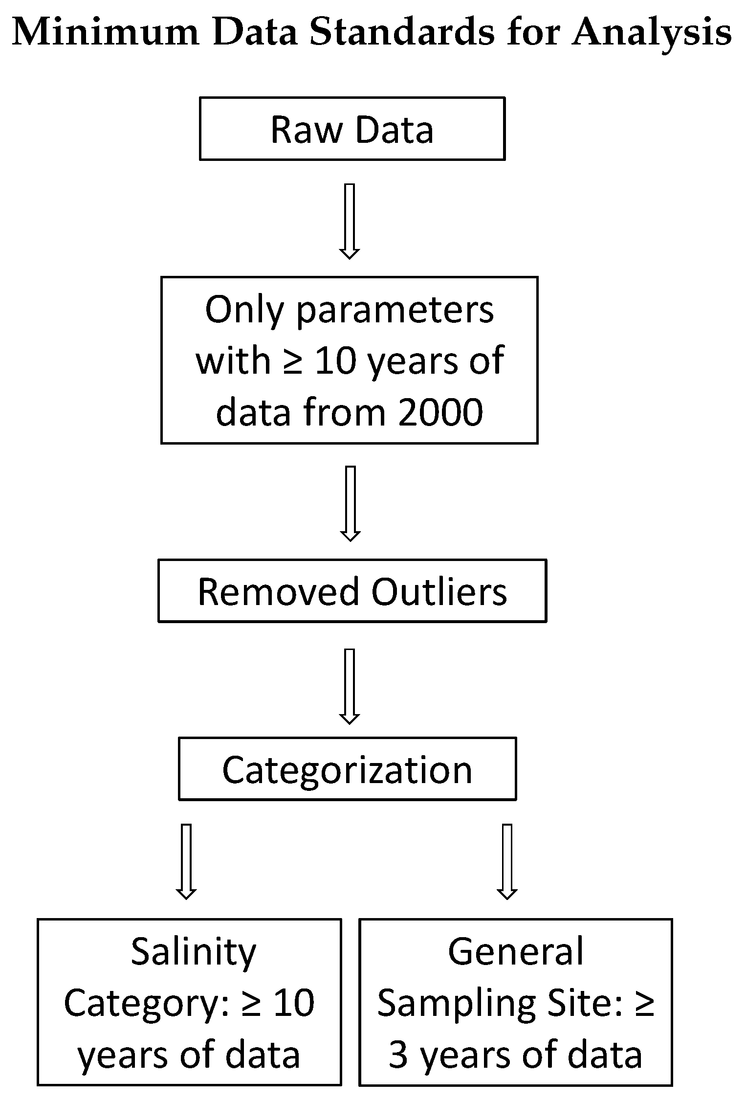
2.3. Analysis
3. Results
3.1. Collation
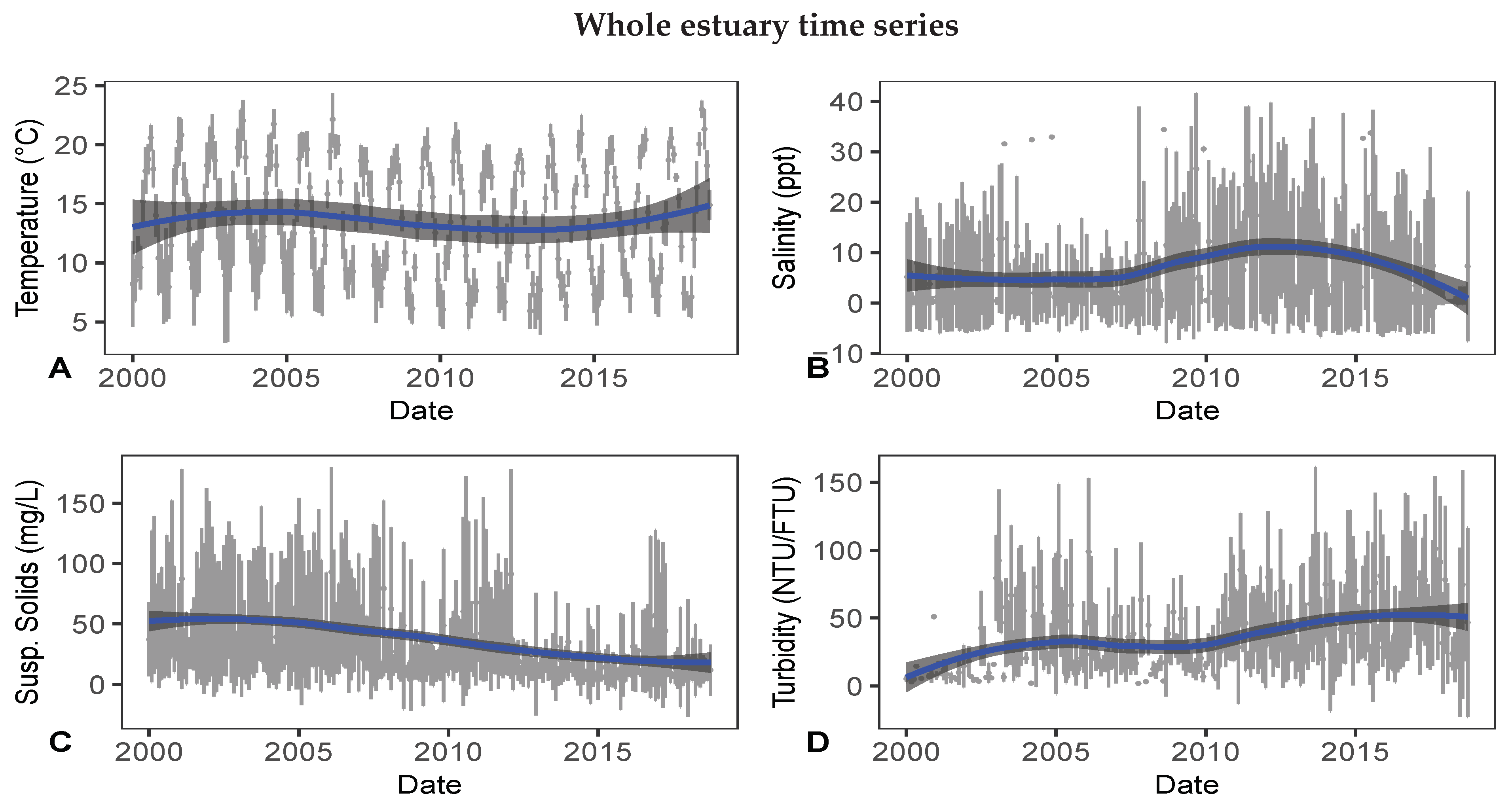
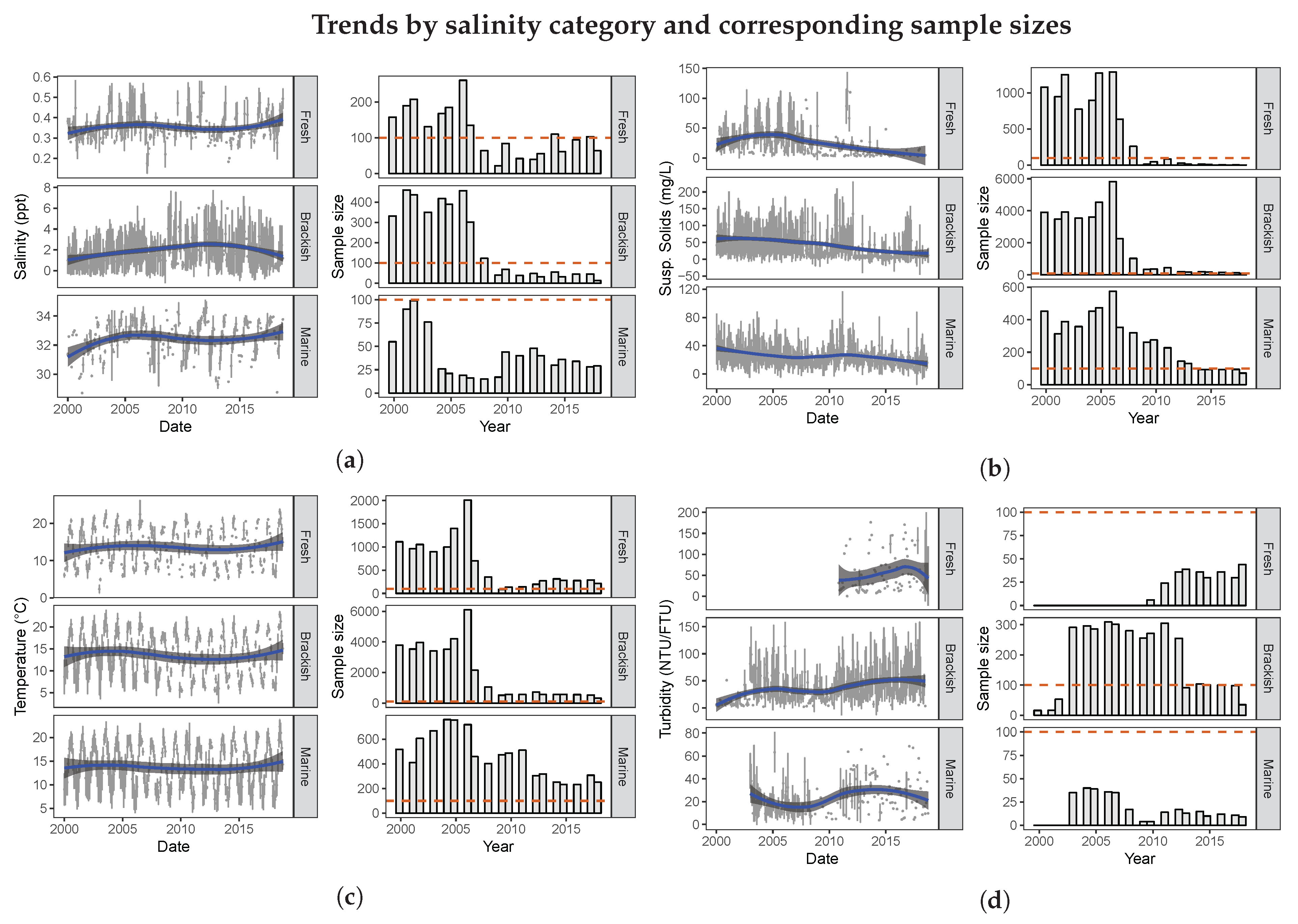
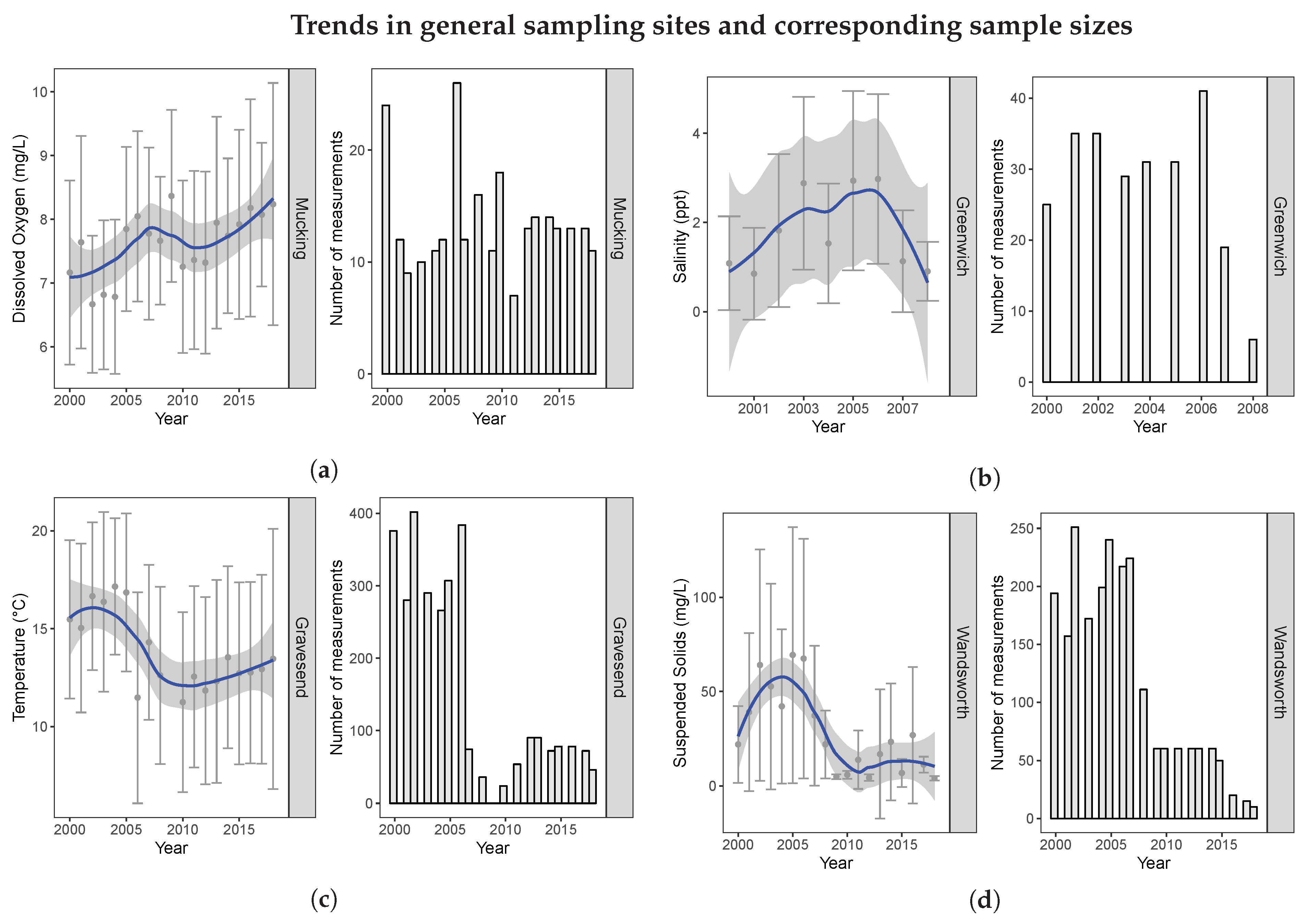
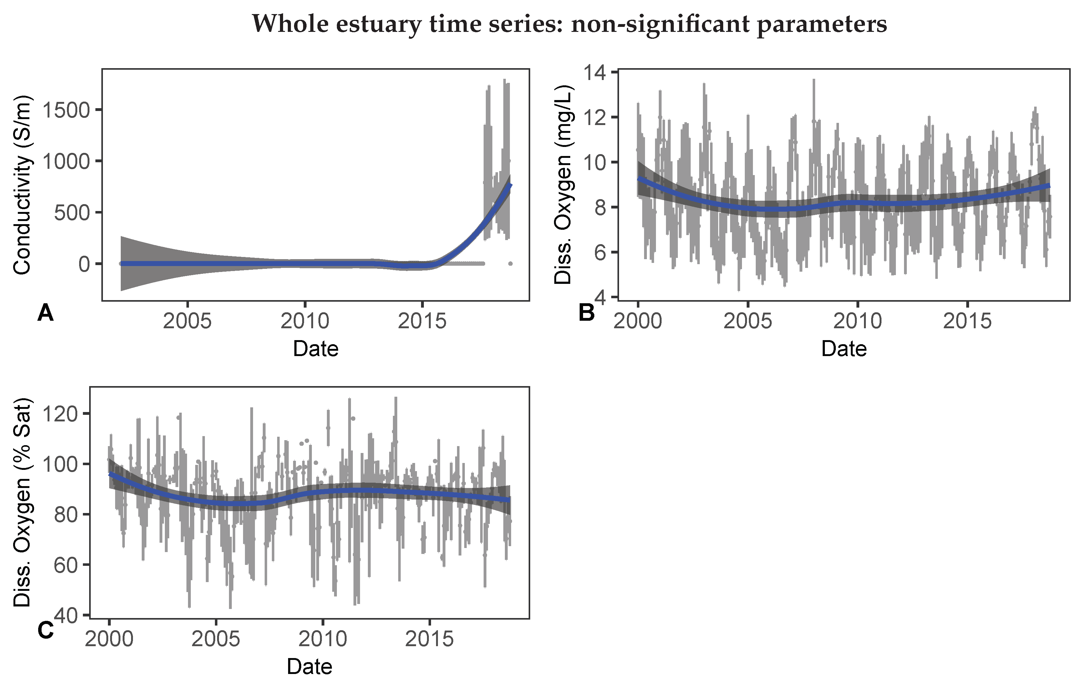
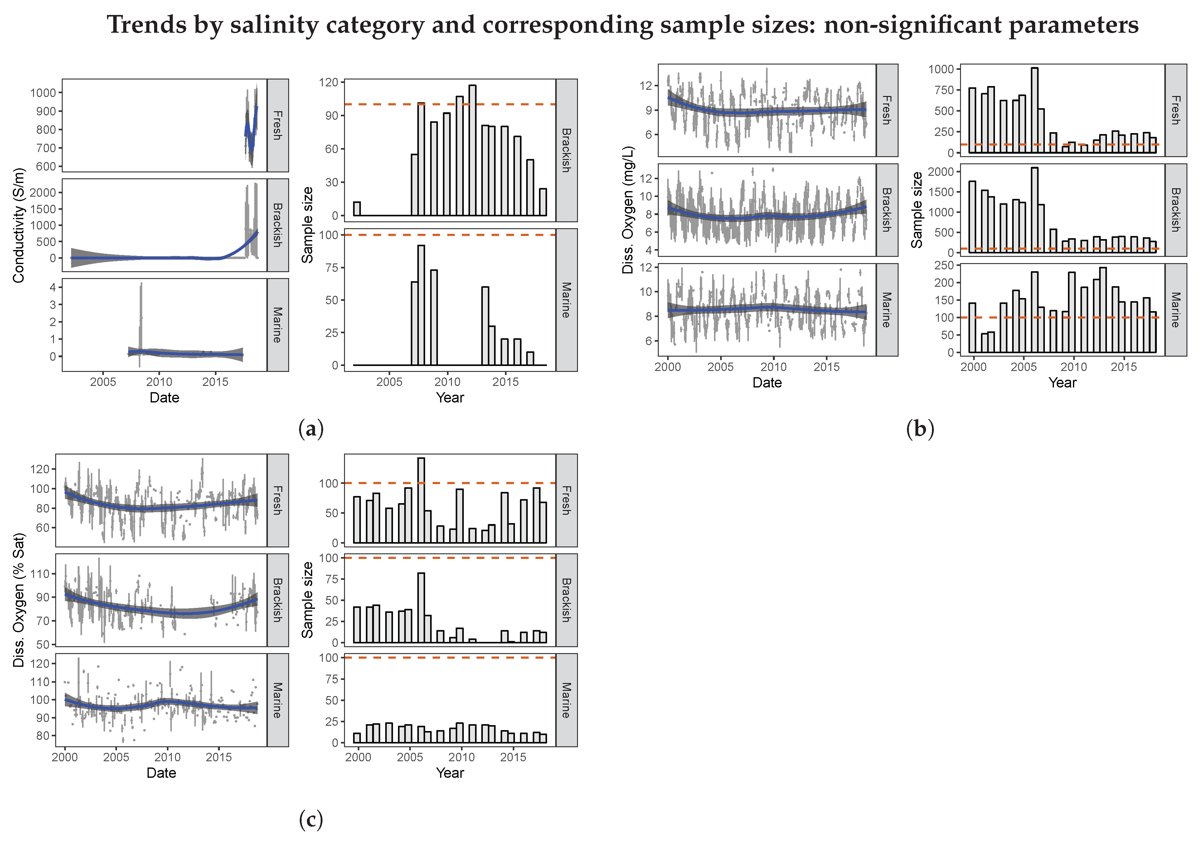
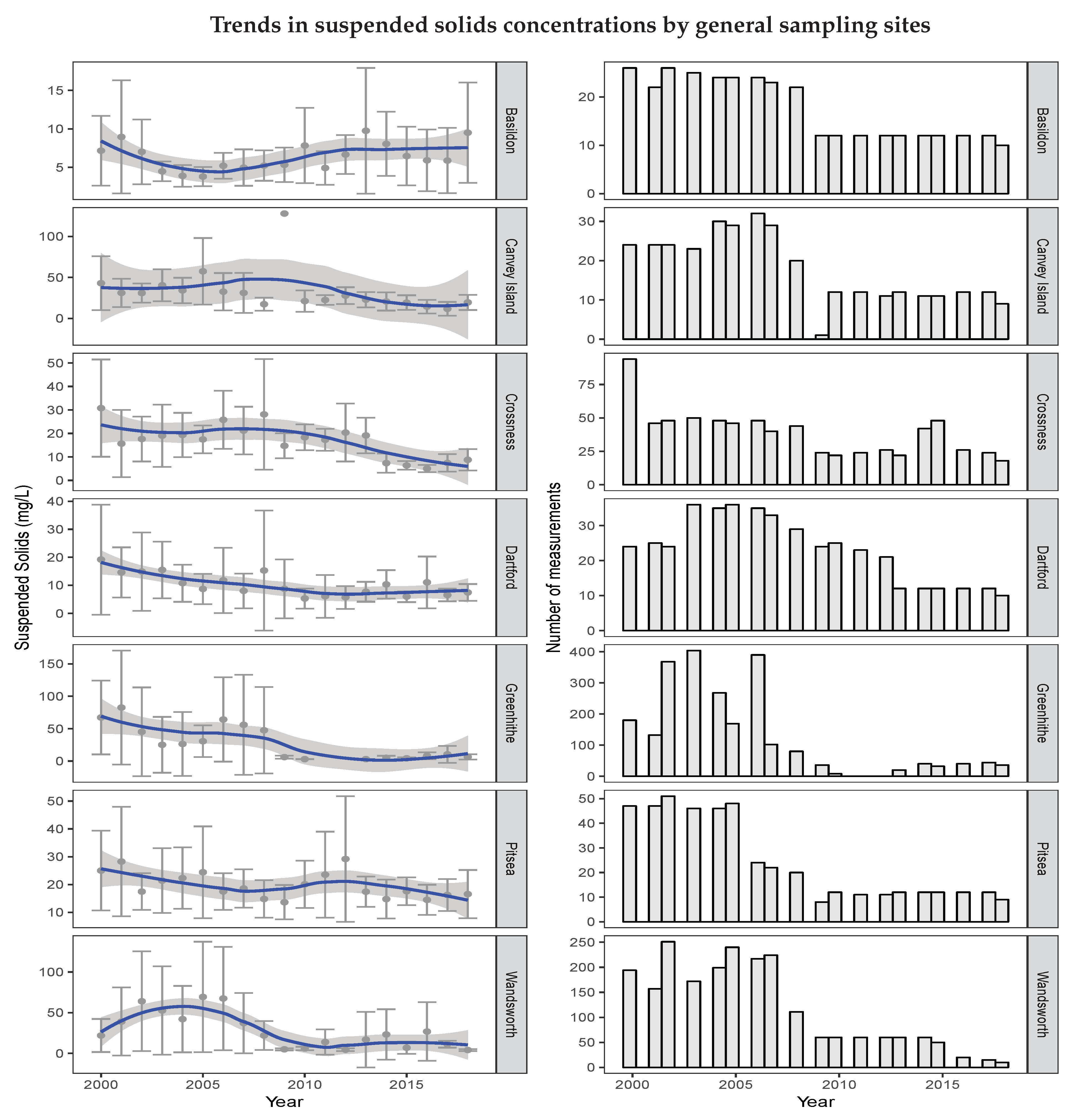
3.2. Seasonal Mann–Kendall
4. Discussion
- Metadata must have defined minimum standards. These standards should include information on instrumentation, tidal cycles, sampling depth, and background on the monitoring program.
- Data should be stored in a centralized data system to increase availability and accessibility, promote standardization and quality control, and provide a standard which can be applied nationally. Examples of this data structure can be seen in the National Estuarine Research Reserve (NERR) system in the United States [73,74] and the South African Environmental Observation Network (SAEON) in South Africa [18,75]. In both programs, centralized databases are established in conjunction with national monitoring programs to ensure data are collected consistently and the database is maintained by frequent checks for quality control.
- Basic physical parameters, such as temperature, salinity, dissolved oxygen, and suspended solids, should be consistently monitored [38]. These parameters have been ignored in monitoring on the Thames, creating a data gap which must be filled as these parameters influence the structure and function of the Thames.
- Future monitoring programs should be guided by question-driven study design. Question-driven designs often involve the creation of a conceptual model which can lead to the formation of hypotheses. This can, in turn, lead to a better understanding of ecosystems through hypothesis-testing instead of only accumulating data points. This opens opportunities for additional research questions and encourages partnerships between other organizations [17].
5. Conclusions
Funding
Acknowledgments
Conflicts of Interest
Appendix A


References
- Fischer, F.; Pellow, D. Citizens, Experts, and the Environment: The Politics of Local Knowledge. Contemp. Sociol. 2002, 31, 578. [Google Scholar] [CrossRef]
- Mayo, E.; Steinburg, T. The Power of Information: An Independent Review. Available online: http://www.opsi.gov.uk/advice/poi/power-ofinformation-review.pdf (accessed on 20 March 2019).
- Attard, J.; Orlandi, F.; Auer, S. Value creation on open government data. In Proceedings of the Annual Hawaii International Conference on System Sciences, Kauai, HI, USA, 5–8 January 2016; pp. 2605–2614. [Google Scholar] [CrossRef]
- Silvertown, J. A new dawn for citizen science. Trends Ecol. Evol. 2009, 24, 467–471. [Google Scholar] [CrossRef]
- Carvalho, A. Ideological cultures and media discourses on scientific knowledge: Re-reading news on climate change. Public Underst. Sci. 2007, 16, 223–243. [Google Scholar] [CrossRef]
- Brandt, J.; Gutbrod, M.; Wellnitz, O.; Wolf, L. Plagiarism detection in open access publications. In Proceedings of the 4th International Plagiarism Conference, Newcastle-Upon-Tyne, UK, 21–23 June 2010. [Google Scholar]
- Bautista-Puig, N.; De Filippo, D.; Mauleón, E.; Sanz-Casado, E. Scientific Landscape of Citizen Science Publications: Dynamics, Content and Presence in Social Media. Publications 2019, 7, 12. [Google Scholar] [CrossRef]
- Theobald, E.; Burgess, H.; Ettinger, A.; Froehlich, H.; HilleRisLambers, J.; DeBey, L.; Wagner, C.; Schmidt, N.; Harsch, M.; Tewksbury, J.; et al. Global change and local solutions: Tapping the unrealized potential of citizen science for biodiversity research. Biol. Conserv. 2014, 181, 236–244. [Google Scholar] [CrossRef]
- Leonelli, S.; Spichtinger, D.; Prainsack, B. Sticks and carrots: Encouraging open science at its source. Geo Geogr. Environ. 2015, 2, 12–16. [Google Scholar] [CrossRef] [PubMed]
- European Commission. Directorate-General for Research and Innovation; European Commission: Brussels, Belgium, 2016; Volume 39, pp. 311–316. [Google Scholar] [CrossRef]
- Parrish, J.K.; Burgess, H.; Weltzin, J.F.; Fortson, L.; Wiggins, A.; Simmons, B. Exposing the Science in Citizen Science: Fitness to Purpose and Intentional Design. Integr. Comp. Biol. 2018, 58, 150–160. [Google Scholar] [CrossRef] [PubMed]
- Burgess, J.; Harrison, C.M.; Filius, P. Environmental communication and the cultural politics of environmental citizenship. Environ. Plan. A 1998, 30, 1445–1460. [Google Scholar] [CrossRef]
- Bäckstrand, K. Civic Science for Sustainability: Reframing the Role of Experts, Policy-Makers and Citizens in Environmental Governance. Glob. Environ. Politics 2004, 3, 24–41. [Google Scholar] [CrossRef]
- Ottinger, G. Buckets of resistance: Standards and the effectiveness of citizen science. Sci. Technol. Hum. Values 2010, 35, 244–270. [Google Scholar] [CrossRef]
- Janssen, M.; Charalabidis, Y.; Zuiderwijk, A. Benefits, Adoption Barriers and Myths of Open Data and Open Government. Inf. Syst. Manag. 2012, 29, 258–268. [Google Scholar] [CrossRef]
- Zuiderwijk, A.; Janssen, M.; Choenni, S.; Meijer, R.; Alibaks, R.S. Socio-technical Impediments of Open Data. Electron. J. E-Gov. 2012, 10, 156–172. [Google Scholar] [CrossRef]
- Lindenmayer, D.B.; Likens, G.E. The science and application of ecological monitoring. Biol. Conserv. 2010, 143, 1317–1328. [Google Scholar] [CrossRef]
- Cilliers, G.; Adams, J. Development and implementation of a monitoring programme for South African estuaries. Water SA 2016, 42, 279–290. [Google Scholar] [CrossRef]
- Máchová, R.; Hub, M.; Lnenicka, M. Usability evaluation of open data portals: Evaluating data discoverability from a stakeholders’ perspective. Aslib J. Inf. Manag. 2018, 70, 252–268. [Google Scholar] [CrossRef]
- Kubler, S.; Robert, J.; Neumaier, S.; Umbrich, J.; Le Traon, Y. Comparison of metadata quality in open data portals using the Analytic Hierarchy Process. Gov. Inf. Q. 2018, 35, 13–29. [Google Scholar] [CrossRef]
- Port of London Authority. Maintenance Dredge Protocol and Water Framework Directive Baseline Document. Available online: http://pla.co.uk/assets/r2238afinalmdpbaselinedocument7oct2014.compressed1.pdf (accessed on 1 April 2019).
- Attrill, M.J.; Power, M. Partitioning of temperature resources amongst an estuarine fish assemblage. Estuar. Coast. Shelf Sci. 2004, 61, 725–738. [Google Scholar] [CrossRef]
- Orr, H.; des Clers, S.; Simpson, G.; Hughes, M.; Batterbee, R.; Cooper, L.; Dunbar, M.; Evans, R.; Hannaford, J.; Hannah, D.; et al. Changing Water Temperatures: A Surface Water Archive for England and Wales; BHS Third International Symposium; Managing Consequences of a Changing Global Environment: Newcastle, UK, 2010; pp. 1–8. [Google Scholar]
- Garner, G.; Hannah, D.M.; Sadler, J.P.; Orr, H.G. River temperature regimes of England and Wales: Spatial patterns, inter-annual variability and climatic sensitivity. Hydrol. Process. 2014, 28, 5583–5598. [Google Scholar] [CrossRef]
- Garner, G.; Hannah, D.M.; Watts, G. Climate change and water in the UK: Recent scientific evidence for past and future change. Prog. Phys. Geogr. 2017, 41, 154–170. [Google Scholar] [CrossRef]
- Tidal Thames Fish Conservation. Available online: https://www.zsl.org/conservation/regions/uk-europe/tidal-thames-fish-conservation (accessed on 25 November 2019).
- Eel Conservation. Available online: https://www.zsl.org/conservation/regions/uk-europe/eel-conservation (accessed on 25 November 2019).
- Gilbert, N. Salmons Brook Healthy River Challenge: The Start-Up Performance of Three Constructed Wetlands at Improving Water Quality. Available online: http://www.thames21.org.uk/wp-content/uploads/2013/11/Salmons-Brook-constructed-wetlands-impact-assessment-FINAL.pdf (accessed on 25 November 2019).
- Folini, S.; Lubello, C.; Katsou, E.; Gori, R. Monitoring of Sustainable Drainage Systems in the Salmons Brook Catchment. Available online: http://www.thames21.org.uk/wp-content/uploads/2017/01/Monitoring-of-Sustainable-Drainage-Systems-in-the-Salmons-Brook-Catchmen....pdf (accessed on 25 November 2019).
- Greater Thames Fish Migration Roadmap. Available online: https://thamesestuarypartnership.org/our-projects/greater-thames-estuary-fish-migration-roadmap/ (accessed on 20 December 2019).
- Paerl, H.W. Assessing and managing nutrient-enhanced eutrophication in estuarine and coastal waters: Interactive effects of human and climatic perturbations. Ecol. Eng. 2006, 26, 40–54. [Google Scholar] [CrossRef]
- Elliott, M.; Whitfield, A.K. Challenging paradigms in estuarine ecology and management. Estuar. Coast. Shelf Sci. 2011, 94, 306–314. [Google Scholar] [CrossRef]
- Dittmann, S.; Baring, R.; Baggalley, S.; Cantin, A.; Earl, J.; Gannon, R.; Keuning, J.; Mayo, A.; Navong, N.; Nelson, M.; et al. Drought and flood effects on macrobenthic communities in the estuary of Australia’s largest river system. Estuar. Coast. Shelf Sci. 2015, 165, 36–51. [Google Scholar] [CrossRef]
- Environment Agency Thames Region. The Water Quality of the Tidal Thames. 1997. Available online: http://www.environmentdata.org/archive/ealit:1710 (accessed on 15 July 2019).
- Best, M.; Wither, A.; Coates, S. Dissolved oxygen as a physico-chemical supporting element in the Water Framework Directive. Mar. Pollut. Bull. 2007, 55, 53–64. [Google Scholar] [CrossRef] [PubMed]
- Bauer, J.E.; Bianchi, T.S. Dissolved Organic Carbon Cycling and Transformation; Elsevier Inc.: Amsterdam, The Netherlands, 2012; Volume 5, pp. 7–67. [Google Scholar] [CrossRef]
- Attrill, M.J. (Ed.) A Rehabilitated Estuarine Ecosystem; Springer: Boston, MA, USA, 1998. [Google Scholar] [CrossRef]
- Borja, A.; Basset, A.; Bricker, S.; Dauvin, J.C.; Elliot, M.; Harrison, T.; Marques, J.; Weisberg, S.; West, R. Classifying ecological quality and integrity of estuaries. Treatise Estuar. Coast. Sci. 2012, 125–162. [Google Scholar] [CrossRef]
- Ross, A.C.; Najjar, R.G.; Li, M.; Mann, M.E.; Ford, S.E.; Katz, B. Sea-level rise and other influences on decadal-scale salinity variability in a coastal plain estuary. Estuar. Coast. Shelf Sci. 2015, 157, 79–92. [Google Scholar] [CrossRef]
- Robins, P.E.; Skov, M.W.; Lewis, M.J.; Giménez, L.; Davies, A.G.; Malham, S.K.; Neill, S.P.; McDonald, J.E.; Whitton, T.A.; Jackson, S.E.; et al. Impact of climate change on UK estuaries: A review of past trends and potential projections. Estuar. Coast. Shelf Sci. 2016, 169, 119–135. [Google Scholar] [CrossRef]
- Frost, M.; Bayliss-Brown, G.; Buckley, P.; Cox, M.; Dye, S.R.; Sanderson, W.G.; Stoker, B.; Withers Harvey, N. A review of climate change and the implementation of marine biodiversity legislation in the United Kingdom. Aquat. Conserv. Mar. Freshw. Ecosyst. 2016, 26, 576–595. [Google Scholar] [CrossRef]
- Jonkers, A.R.; Sharkey, K.J. The differential warming response of Britain’s rivers (1982–2011). PLoS ONE 2016, 11, e0166247. [Google Scholar] [CrossRef]
- Werner, A.D.; Simmons, C.T. Impact of sea-level rise on sea water intrusion in coastal aquifers. Groundwater 2009, 47, 197–204. [Google Scholar] [CrossRef]
- Veríssimo, H.; Lane, M.; Patrício, J.; Gamito, S.; Marques, J.C. Trends in water quality and subtidal benthic communities in a temperate estuary: Is the response to restoration efforts hidden by climate variability and the Estuarine Quality Paradox? Ecol. Indic. 2013, 24, 56–67. [Google Scholar] [CrossRef]
- Werner, A.D.; Bakker, M.; Post, V.E.; Vandenbohede, A.; Lu, C.; Ataie-Ashtiani, B.; Simmons, C.T.; Barry, D.A. Seawater intrusion processes, investigation and management: Recent advances and future challenges. Adv. Water Resour. 2013, 51, 3–26. [Google Scholar] [CrossRef]
- McLeod, A. Kendall: Kendall Rank Correlation and Mann–Kendall Trend Test, R Package Version 2.2; 2011. Available online: https://CRAN.R-project.org/package=Kendall (accessed on 15 July 2019).
- R Core Team. R: A Language and Environment for Statistical Computing; R Foundation for Statistical Computing: Vienna, Austria, 2018. [Google Scholar]
- Hirsch, R.M.; Slack, J.R.; Smith, R.A. Techniques for trend assessment for monthly water quality data. Water Resour. Res. 1982, 18, 107–121. [Google Scholar] [CrossRef]
- Hirsch, R.M.; Slack, J.R. A Nonparametric Trend Test for Seasonal Data with Serial Dependence. Water Resour. 1984, 20, 727–732. [Google Scholar] [CrossRef]
- Kosanic, A.; Harrison, S.; Anderson, K.; Kavcic, I. Present and historical climate variability in South West England. Clim. Chang. 2014, 124, 221–237. [Google Scholar] [CrossRef]
- Kahya, E.; Kalaycı, S. Trend analysis of streamflow in Turkey. J. Hydrol. 2004, 289, 128–144. [Google Scholar] [CrossRef]
- Levinton, J.S.; Levinton, J.S. Marine Biology: Function, Biodiversity, Ecology; Oxford University Press: New York, NY, USA, 1995; Volume 420. [Google Scholar]
- Francis, R.A.; Hoggart, S.P.; Gurnell, A.M.; Coode, C. Meeting the challenges of urban river habitat restoration: Developing a methodology for the River Thames through central London. Area 2008, 40, 435–445. [Google Scholar] [CrossRef]
- Boyd, S.E.; Limpenny, D.S.; Rees, H.L.; Cooper, K.M. The effects of marine sand and gravel extraction on the macrobenthos at a commercial dredging site (results 6 years post-dredging). ICES J. Mar. Sci. 2005, 62, 145–162. [Google Scholar] [CrossRef]
- Nicholson, A.; Meakins, N.; Mcnulty, S.; Pieris, M. Dredging Conservation Assessment for the Thames Estuary Status Final Report. Available online: https://www.pla.co.uk/assets/9t7480dredgingconservationassessmentupdatefinalversion.pdf (accessed on 1 April 2019).
- Taylor, V. London’s River? The Thames as Contested Environmental Space. Lond. J. 2015, 40, 183–195. [Google Scholar] [CrossRef]
- Jones, H.P.; Schmitz, O.J. Rapid recovery of damaged ecosystems. PLoS ONE 2009, 4, e5653. [Google Scholar] [CrossRef]
- Borja, Á.; Dauer, D.M.; Elliott, M.; Simenstad, C.A. Medium-and Long-term Recovery of Estuarine and Coastal Ecosystems: Patterns, Rates and Restoration Effectiveness. Estuaries Coasts 2010, 33, 1249–1260. [Google Scholar] [CrossRef]
- Sokal, R.R.; Rohlf, F.J. Biometry; Freeman Co.: San Francisco, CA, USA, 1981; p. 776. [Google Scholar]
- Water Quality Data Archive. Available online: https://environment.data.gov.uk/water-quality/view/landing (accessed on 8 January 2019).
- Colclough, S.; Gray, G.; Bark, A.; Knights, B. Fish and fisheries of the tidal Thames: Management of the modern resource, research aims and future pressures. J. Fish Biol. 2002, 61, 64–73. [Google Scholar] [CrossRef]
- Thorson, J.T.; Jensen, O.P.; Hilborn, R. Probability of stochastic depletion: An easily interpreted diagnostic for stock assessment modelling and fisheries management. ICES J. Mar. Sci. 2015, 72, 428–435. [Google Scholar] [CrossRef]
- Voulvoulis, N.; Arpon, K.D.; Giakoumis, T. The EU Water Framework Directive: From great expectations to problems with implementation. Sci. Total Environ. 2017, 575, 358–366. [Google Scholar] [CrossRef] [PubMed]
- Borja, A.; Elliott, M.; Henriksen, P.; Marbà, N. Transitional and coastal waters ecological status assessment: Advances and challenges resulting from implementing the European Water Framework Directive. Hydrobiologia 2013, 704, 213–229. [Google Scholar] [CrossRef]
- UKTAG. UK Environmental Standards and Conditions (Phase 1). Available online: https://www.wfduk.org/sites/default/files/Media/Environmental standards/Environmental standards phase 1_Finalv2_010408.pdf (accessed on 29 July 2019).
- UKTAG. UK Environmental Standards and Conditions (Phase 2). Available online: https://www.wfduk.org/sites/default/files/Media/Environmental standards/Environmental standards phase 2_Final_110309.pdf (accessed on 30 July 2019).
- Collins, A.; Ohandja, D.G.; Hoare, D.; Voulvoulis, N. Implementing the Water Framework Directive: A transition from established monitoring networks in England and Wales. Environ. Sci. Policy 2012, 17, 49–61. [Google Scholar] [CrossRef]
- Borja, Á.; Rodríguez, J.G. Problems associated with the ‘one-out, all-out’ principle, when using multiple. Mar. Pollut. Bull. 2010, 60, 1143–1146. [Google Scholar] [CrossRef]
- Carvalho, L.; Mackay, E.B.; Cardoso, A.C.; Baattrup-Pedersen, A.; Birk, S.; Blackstock, K.L.; Borics, G.; Borja, A.; Feld, C.K.; Ferreira, M.T.; et al. Protecting and restoring Europe’s waters: An analysis of the future development needs of the Water Framework Directive. Sci. Total Environ. 2019, 658, 1228–1238. [Google Scholar] [CrossRef]
- Carstensen, J.; Lindegarth, M. Confidence in ecological indicators: A framework for quantifying uncertainty components from monitoring data. Ecol. Indic. 2016, 67, 306–317. [Google Scholar] [CrossRef]
- Gamito, R.; Pasquaud, S.; Courrat, A.; Drouineau, H.; Fonseca, V.F.; Gonçalves, C.I.; Wouters, N.; Costa, J.L.; Lepage, M.; Costa, M.J.; et al. Influence of sampling effort on metrics of fish-based indices for the assessment of estuarine ecological quality. Ecol. Indic. 2012, 23, 9–18. [Google Scholar] [CrossRef]
- Van Puijenbroek, P.; Evers, C.; van Gaalen, F. Evaluation of Water Framework Directive metrics to analyse trends in water quality in The Netherlands. Sustain. Water Qual. Ecol. 2015, 6, 40–47. [Google Scholar] [CrossRef]
- Buskey, E.J.; Bundy, M.; Ferner, M.C.; Porter, D.E.; Reay, W.G.; Smith, E.; Trueblood, D. System-wide monitoring program of the National Estuarine Research Reserve System: Research and monitoring to address coastal management issues. In Coastal Ocean Observing Systems; Elsevier: Amsterdam, The Netherlands, 2015; pp. 392–415. [Google Scholar] [CrossRef]
- National Oceanic and Atmospheric Administration. National Estuarine Research Reserve System: System Wide Monitoring Program Plan. Available online: https://coast.noaa.gov/data/docs/nerrs/Research_2011SWMPPlan.pdf (accessed on 28 August 2019).
- Hallett, C.S.; Valesini, F.; Elliott, M. A review of Australian approaches for monitoring, assessing and reporting estuarine condition: I. International context and evaluation criteria. Environ. Sci. Policy 2016, 66, 260–269. [Google Scholar] [CrossRef]


| Data Set | Time Range | Key Parameter Units | Resolution |
|---|---|---|---|
| EA queried | 1989–2018 | Temperature, salinity (ppt, conductivity), dissolved oxygen (mg/L, % saturation), turbidity (Nephelometric Turbidity Units (NTU)/Formazin Turbidity Unit (FTU), suspended solids). | Daily, weekly, or monthly |
| WIMS | 2000–2018 | Temperature, salinity (ppt, conductivity), dissolved oxygen (mg/L, % saturation), turbidity (NTU/FTU, suspended solids). | Weekly |
| AQMS | 2017–2018 | Temperature, salinity (ppt, conductivity), dissolved oxygen (mg/L), turbidity (NTU/FTU). | Fifteen minute intervals |
| Parameter | p-Value | |
|---|---|---|
| Temperature (°C) | −0.247 | 5.19 × 10⁻⁷ |
| Salinity (ppt) | 0.104 | 0.0352 |
| Suspended Solids (mg/L) | −0.457 | <2.22 × 10⁻⁶ |
| Turbidity (NTU/FTU) | 0.328 | 2.80 × 10⁻¹¹ |
| Conductivity (S/m) | −0.0587 | 0.234 |
| Dissolved Oxygen (mg/L) | 0.0388 | 0.431 |
| Dissolved Oxygen (% sat) | −0.021 | 0.671 |
| Parameter | Salinity Category | p-Value | |
|---|---|---|---|
| Temperature (°C) | Fresh | 0.053 | 0.278 |
| Brackish | −0.271 | 3.63 × 10⁻⁸ | |
| Marine | −0.171 | 5.27 × 10⁻⁴ | |
| Salinity (ppt) | Fresh | 0.034 | 0.496 |
| Brackish | 0.145 | 3.34 × 10⁻³ | |
| Marine | 0.045 | 0.360 | |
| Suspended Solids (mg/L) | Fresh | −0.155 | 1.65 × 10⁻³ |
| Brackish | −0.420 | <0.001 | |
| Marine | −0.402 | 2.22 × 10⁻¹⁶ | |
| Turbidity (NTU/FTU) | Fresh | 0.039 | 0.425 |
| Brackish | 0.276 | 2.23 × 10⁻⁸ | |
| Marine | −0.0503 | 0.307 | |
| Conductivity (S/m) | Fresh | 0.0363 | 0.468 |
| Brackish | 0.0210 | 0.671 | |
| Marine | 0.00238 | 0.963 | |
| Dissolved Oxygen (mg/L) | Fresh | −0.0314 | 0.523 |
| Brackish | 0.0608 | 0.217 | |
| Marine | −0.0514 | 0.297 | |
| Dissolved Oxygen (% sat) | Fresh | 0.0126 | 0.799 |
| Brackish | −0.0367 | 0.457 | |
| Marine | −0.0288 | 0.559 |
| Parameter | General Sampling Site | p-Value | |
|---|---|---|---|
| Dissolved Oxygen (mg/L) | Mucking | 0.105 | 0.0334 |
| Salinity (ppt) | Greenwich | 0.180 | 0.0268 |
| Temperature (°C) | Gravesend | −0.126 | 0.0107 |
| Suspended Solids (mg/L) | Basildon | 0.115 | 0.0211 |
| Canvey Island | −0.217 | 1.24 × 10⁻⁵ | |
| Crossness | −0.288 | 5.76 × 10⁻⁹ | |
| Dartford | −0.298 | 1.54 × 10⁻⁹ | |
| Greenhithe | −0.164 | 8.98 × 10⁻⁴ | |
| Pitsea | −0.129 | 9.32 × 10⁻³ | |
| Wandsworth | −0.130 | 8.34 × 10⁻³ |
© 2020 by the author. Licensee MDPI, Basel, Switzerland. This article is an open access article distributed under the terms and conditions of the Creative Commons Attribution (CC BY) license (http://creativecommons.org/licenses/by/4.0/).
Share and Cite
Lanoue, J. Disparate Environmental Monitoring as a Barrier to the Availability and Accessibility of Open Access Data on the Tidal Thames. Publications 2020, 8, 6. https://doi.org/10.3390/publications8010006
Lanoue J. Disparate Environmental Monitoring as a Barrier to the Availability and Accessibility of Open Access Data on the Tidal Thames. Publications. 2020; 8(1):6. https://doi.org/10.3390/publications8010006
Chicago/Turabian StyleLanoue, Julia. 2020. "Disparate Environmental Monitoring as a Barrier to the Availability and Accessibility of Open Access Data on the Tidal Thames" Publications 8, no. 1: 6. https://doi.org/10.3390/publications8010006
APA StyleLanoue, J. (2020). Disparate Environmental Monitoring as a Barrier to the Availability and Accessibility of Open Access Data on the Tidal Thames. Publications, 8(1), 6. https://doi.org/10.3390/publications8010006