Deep Learning-Based Robust Visible Light Positioning for High-Speed Vehicles

 and
and 
Abstract
:1. Introduction
2. The Proposed DL-Based Robust VLP Systems
2.1. System Architecture
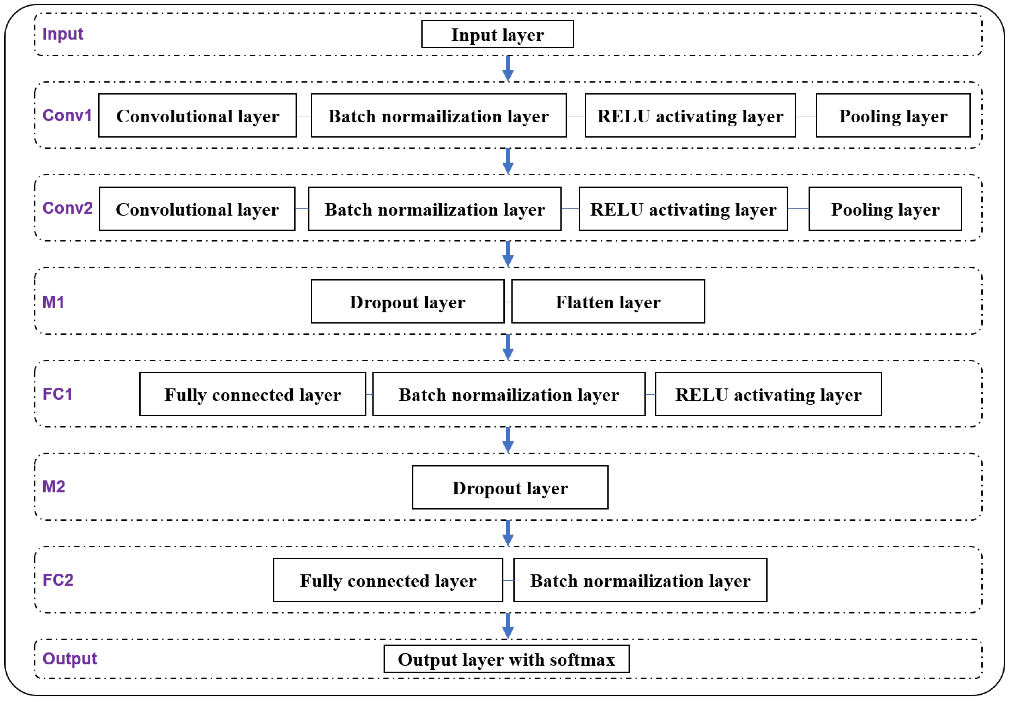
2.2. The Proposed DL-Based Decoder with BN-CNN
- 1
- The first layer is the Input layer, which is read in VLP-LED stripe images with the size of 800 × 800 pixels.
- 2
- In Layer Conv1, the convolutional layer uses 32 convolutional kernels of 3 × 3 size with the step of (1, 1) to extract features and generate 32 feature maps. Let the input array be and the output array be , then, the convolutional layer performs the extraction of feature maps according to the following equation.where is the bias of the neuron, is the weight of the neuron, and * denotes the convolution operations.After the feature mapping in the convolutional layer, we use zero to fill the edge pixels of the 798 × 798 feature maps and obtain 32 feature maps with the size of 800 × 800. A batch normalization layer is utilized to normalize the feature maps output from the convolution layer and then the average value and variance of the feature maps are limited to the range of [0, 1]. It helps accelerate the convergence speed of the proposed BN-CNN model and improve the generalization ability of the model.Here, the batch normalization layer introduces the mean and variance of each batch into the convolutional neural network, while the mean and variance of different batches are generally different. Therefore, the batch normalization layer is equivalent to adding random noise to the process of convolutional neural network training, which can play a role in preventing model overfitting. On the other hand, the batch normalization layer adjusts the input of any neuron of the neural network to a standard normal distribution with mean 0 and variance 1, so that the input value of the activation layer falls in the region where the nonlinear function is more sensitive to the input, i.e., a smaller input change leads to a larger gradient change, which avoids the vanishing gradient problem and speeds up the convergence of the neural network.Further, with the excitation function of the RELU activating layer, the output of the batch normalization layer is mapped nonlinearly into the max pooling layer in Layer Conv1. The max pooling layer uses a max pooling with the step of (2, 2) to calculate and output the maximum value of the data corresponding to the sliding process of the polling window. The max pooling layer implements a separate dimensionality reduction of each feature map to reduce the connection between layers, as well as the amount of data to be computed and stored. It also reduces the risk of model overfitting. After the max pooling layer, the size of the output feature map is reduced to 400 × 400.
- 3
- Layer Conv2 has a similar structure to that of Layer Conv1, while it employs 64 convolutional kernels of 3 × 3 size with the step of (1, 1) to further extract higher-dimension features from the 32 feature maps generated by Layer Conv1 and to generate 64 feature maps. After the batch normalization layer, RELU activation layer and max pooling layer in Layer Conv2, 64 feature maps with the size of 200 × 200 will be generated for next processing.
- 4
- In Layer M1, the dropout layer is introduced to randomly discardsome hidden neurons to avoid overfitting of the training model. Through randomly discarding 50% of hidden neurons during forward propagation, the dropout layer can reduce the complex co-adaptive relationships between neurons and avoid relying on the linkage relationships between neurons. As a result, the dropout layer can alleviate the occurrence of overfitting and improve the robustness of CNN training. Additionally, randomly discarding some neurons in the network is equivalent to averaging over many different neural networks and it can significantly improve the generalization ability of the CNN model.After the dropout layer, the flatten layer transforms the 64 × 200 × 200 feature maps into a 64 × 200 × 200 one-dimensional feature array, which will be fed into the fully connected layer.
- 5
- In Layer FC1, the fully connected layer uses 512 connected nodes to convert the input feature array into 512 scored values, which are propagated forward to the batch normalization layer. The batch normalization layer is used to adjust the input of the RELU activation layer to a standard normal distribution, which can speed up network training and prevent the vanishing gradient problem. The normalized scored values are input into the RELU activation layer to add nonlinear factors into the neural network, which makes the neural network can adapt to more complex problems.
- 6
- Layer M2 only contains a dropout layer, which is used to further reduce the co-adaptive relationship between the neurons of the neural network. There is no need for adding a flatten layer between layer FC1 and layer FC2.
- 7
- Layer FC2 uses a fully connected layer and a batch normalization layer, as in the layer FC1. After the last fully connected layer with the number of connected nodes of N, the feature values are finally output as N classification results corresponding to N LED-UIDs.
- 8
- Finally, we input the N classification outputs from layer FC2 to the Output layer. In order to obtain the accurate results of the 9 classification outputs for backpropagation and simplify the calculation of the loss function, we use softmax to calculate in the output layer. The output layer uses a softmax classifier to convert the N classification outputs into a classification percentage that sums to 1. The softmax classifier equation is:is the ith input signal in the output layer, the denominator indicates that there are j output signals (neurons) in the output layer, and the exponential sum of all the input signals in the output layer is calculated. is the output of the ith neuron, and the formula is used to calculate the probability distribution of the original input image data after feature extraction of the convolutional neural network to finally obtain the closest to each identifier. The probability distribution is then used in the classifier to obtain the loss value L of the current model calculated according to Equation (3) to back-propagate the convolution kernel (weight matrix) of the optimized convolution layer so that the loss value L keeps decreasing.
2.3. Lightweight Fast ROI Detection Algorithm for Extracting VLP-LED Stripe Images
- 1
- First, the captured image is scanned from left to right with an initial step length (denoted as la, which is 9 pixels in this paper) to detect whether the column under scanning contains enough number of bright pixels. If so, the column is inside a VLP-LED stripe image region since the low exposure setting of the CMOS camera makes sure that only the VLP-LED stripe image region contains bright pixels;
- 2
- Then, from the “bright” column which is detected, we use a smaller step length, denoted as lb, which is 1 pixel in this paper)to scan the image back and forth to precisely determine the left edge and the right edge of the VLP-LED stripe image region;
- 3
- Similarly, the upper edge and the lower edge of the VLP-LED stripe image region can be determined. The VLP-LED stripe image can also be extracted, as shown in Figure 5.
3. Experimental Results
3.1. Experimental Setup
3.2. Success Rate of UID Decoding for Normal Clear Images
3.3. Success Rate of UID Decoding for Motion-Blurred Images
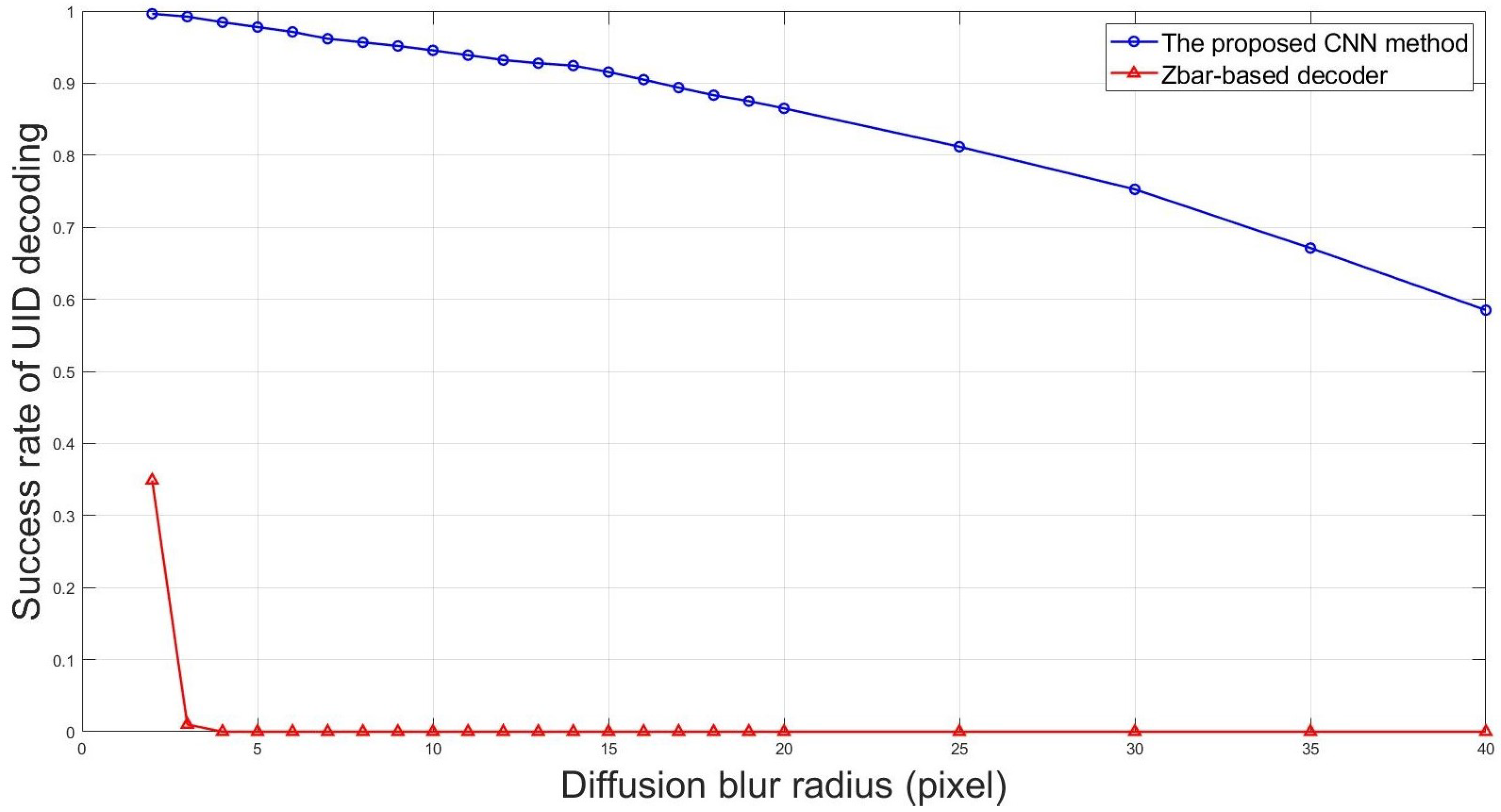
3.4. Success Rate of UID Decoding for Diffusion-Blurred Images
3.5. Positioning Time
4. Conclusions
Author Contributions
Funding
Data Availability Statement
Conflicts of Interest
References
- He, J.; Zhou, B. Vehicle positioning scheme based on visible light communication using a CMOS camera. Opt. Express 2021, 29, 27278–27290. [Google Scholar] [CrossRef] [PubMed]
- Guan, W.; Chen, S.; Wen, S.; Tan, Z.; Song, H.; Hou, W. High-accuracy robot indoor localization scheme based on robot operating system using visible light positioning. IEEE Photonics J. 2020, 12, 7901716. [Google Scholar] [CrossRef]
- Hussain, B.; Wang, Y.; Chen, R.; Cheng, H.; Yue, C. LiDR: Visible Light Communication-Assisted Dead Reckoning for Accurate Indoor Localization. IEEE Internet Things J. 2022, 9, 15742–15755. [Google Scholar] [CrossRef]
- Armstrong, J.; Sekercioglu, Y.A.; Neild, A. Visible light positioning: A roadmap for international standardization. IEEE Commun. Mag. 2013, 51, 68–73. [Google Scholar] [CrossRef]
- Yasir, M.; Ho, S.W.; Vellambi, B.N. Indoor position tracking using multiple optical receivers. J. Lightwave Technol. 2015, 34, 1166–1176. [Google Scholar] [CrossRef]
- Steendam, H. A 3-D positioning algorithm for AOA-based VLP with an aperture-based receiver. IEEE J. Sel. Areas Commun. 2017, 36, 23–33. [Google Scholar] [CrossRef]
- Wu, Y.C.; Chow, C.W.; Liu, Y.; Lin, Y.S.; Hong, C.Y.; Lin, D.C.; Song, S.H.; Yeh, C.H. Received-signal-strength (RSS) based 3D visible-light-positioning (VLP) system using kernel ridge regression machine learning algorithm with sigmoid function data preprocessing method. IEEE Access 2020, 8, 214269–214281. [Google Scholar] [CrossRef]
- Meng, X.; Jia, C.; Cai, C.; He, F.; Wang, Q. Indoor High-Precision 3D Positioning System Based on Visible-Light Communication Using Improved Whale Optimization Algorithm. Photonics 2022, 9, 93. [Google Scholar] [CrossRef]
- Martínez-Ciro, R.A.; López-Giraldo, F.E.; Luna-Rivera, J.M.; Ramírez-Aguilera, A.M. An Indoor Visible Light Positioning System for Multi-Cell Networks. Photonics 2022, 9, 146. [Google Scholar] [CrossRef]
- You, X.; Yang, X.; Jiang, Z.; Zhao, S. A Two-LED Based Indoor Three-Dimensional Visible Light Positioning and Orienteering Scheme for a Tilted Receiver. Photonics 2022, 9, 159. [Google Scholar] [CrossRef]
- Zhu, B.; Zhu, Z.; Wang, Y.; Cheng, J. Optimal optical omnidirectional angle-of-arrival estimator with complementary photodiodes. J. Lightwave Technol. 2019, 37, 2932–2945. [Google Scholar] [CrossRef]
- Do, T.H.; Yoo, M. An in-depth survey of visible light communication based positioning systems. Sensors 2019, 16, 678. [Google Scholar] [CrossRef] [PubMed]
- Hsu, C.W.; Liu, S.; Lu, F.; Chow, C.W.; Yeh, C.H.; Chang, G.K. Accurate indoor visible light positioning system utilizing machine learning technique with height tolerance. In Proceedings of the 2018 Optical Fiber Communications Conference and Exposition (OFC), San Diego, CA, USA, 11–15 March 2018; Volume 3, pp. 1–3. [Google Scholar]
- Chuang, Y.C.; Li, Z.Q.; Hsu, C.W.; Liu, Y.; Chow, C.W. Visible light communication and positioning using positioning cells and machine learning algorithms. Opt. Express 2019, 27, 16377–16383. [Google Scholar] [CrossRef] [PubMed]
- Lin, P.; Hu, X.; Ruan, Y.; Li, H.; Fang, J.; Zhong, Y.; Zheng, H.; Fang, J.; Jiang, Z.L.; Chen, Z. Real-time visible light positioning supporting fast moving speed. Opt. Express 2020, 28, 14503–14510. [Google Scholar] [CrossRef]
- Li, H.; Huang, H.; Xu, Y.; Wei, Z.; Yuan, S.; Lin, P.; Wu, H.; Lei, W.; Fang, J.; Chen, Z. A fast and high-accuracy real-time visible light positioning system based on single LED lamp with a beacon. IEEE Photonics J. 2020, 12, 7906512. [Google Scholar] [CrossRef]
- Guan, W.; Huang, L.; Wen, S.; Yan, Z.; Liang, W.; Yang, C.; Liu, Z. Robot Localization and Navigation Using Visible Light Positioning and SLAM Fusion. J. Lightwave Technol. 2021, 39, 7040–7051. [Google Scholar] [CrossRef]
- Lin, D.C.; Chow, C.W.; Peng, C.W.; Hung, T.Y.; Chang, Y.H.; Song, S.H.; Lin, Y.S.; Lin, Y.; Lin, K.H. Positioning unit cell model duplication with residual concatenation neural network (RCNN) and transfer learning for visible light positioning (VLP). J. Lightwave Technol. 2021, 39, 6366–6372. [Google Scholar] [CrossRef]
- Xie, C.; Guan, W.; Wu, Y.; Fang, L.; Cai, Y. The LED-ID detection and recognition method based on visible light positioning using proximity method. IEEE Photonics J. 2018, 10, 7902116. [Google Scholar] [CrossRef]
- Guan, W.; Chen, X.; Huang, M.; Liu, Z.; Wu, Y.; Chen, Y. High-speed robust dynamic positioning and tracking method based on visual visible light communication using optical flow detection and Bayesian forecast. IEEE Photonics J. 2018, 10, 7904722. [Google Scholar] [CrossRef]
- Su, S.; Heidrich, W. Rolling shutter motion deblurring. In Proceedings of the IEEE Conference on Computer Vision and Pattern Recognition, Boston, MA, USA, 7–12 June 2015; pp. 1529–1537. [Google Scholar]
- Schöberl, M.; Fößel, S.; Bloss, H.; Kaup, A. Modeling of image shutters and motion blur in analog and digital camera systems. In Proceedings of the 2009 16th IEEE International Conference on Image Processing (ICIP), Cairo, Egypt, 7–10 November 2009. [Google Scholar]
- Ioffe, S.; Szegedy, C. Batch normalization: Accelerating deep network training by reducing internal covariate shift. In Proceedings of the International Conference on Machine Learning (ICML), Lile, France, 6–11 July 2015; pp. 448–456. [Google Scholar]
- Santurkar, S.; Tsipras, D.; Ilyas, A.; Mądry, A. How does batch normalization help optimization? In Proceedings of the 32nd International Conference on Neural Information Processing Systems (NIPS’18), Montréal, QC, Canada, 3–8 December 2018; pp. 2488–2498. [Google Scholar]
- ZBar Bar Code Reader. Available online: http://zbar.sourceforge.net/ (accessed on 29 June 2022).
- Lin, H.Y.; Li, K.J.; Chang, C.H. Vehicle speed detection from a single motion blurred image. Image Vis. Comput. 2008, 26, 21327–21337. [Google Scholar] [CrossRef]
- Xu, T.-F.; Zho, P. Object’s translational speed measurement using motion blur information. Measurement 2010, 43, 1173–1179. [Google Scholar]
- Mohammadi, J.; Akbari, R. Vehicle speed estimation based on the image motion blur using radon transform. In Proceedings of the 2010 2nd International Conference on Signal Processing Systems (ICSPS), Dalian, China, 5–7 July 2010. V1-243. [Google Scholar]
- Orieux, F.; Giovannelli, J.F.; Rodet, T. Bayesian estimation of regularization and point spread function parameters for Wiener–Hunt deconvolution. J. Opt. Soc. Am. A 2010, 27, 1593–1607. [Google Scholar] [CrossRef] [PubMed] [Green Version]


| UID Decoding Method | Success Rate |
|---|---|
| The proposed BN-CNN for 1440 images in train set | 99.9% |
| The proposed BN-CNN for 360 images in test set | 99.2% |
| Zbar-based decoder for 1800 images in data set | 99.9% |
| Diagonal Motion Blur Length K (Pixel) | (km/h) |
|---|---|
| 2 | 1.5 |
| 3 | 2.3 |
| 4 | 3.0 |
| 5 | 3.8 |
| 6 | 4.6 |
| 7 | 5.4 |
| 8 | 6.2 |
| 9 | 6.9 |
| 10 | 7.7 |
| 11 | 8.5 |
| 12 | 9.2 |
| 13 | 10.0 |
| 14 | 10.7 |
| 15 | 11.5 |
| 20 | 15.4 |
| 25 | 19.2 |
| 30 | 23.1 |
| 35 | 26.9 |
| 40 | 30.8 |
| 45 | 34.6 |
| 50 | 38.5 |
| VLP Algorithm | Used Time of ROI Detection (ms) | Used Time of UID Decoding (ms) | Overall Positioning Time (ms) |
|---|---|---|---|
| DL-based VLP | 1.01 | 8.18 | 9.19 |
| Zbar-based VLP | 1.01 | 98.53 | 99.54 |
Publisher’s Note: MDPI stays neutral with regard to jurisdictional claims in published maps and institutional affiliations. |
© 2022 by the authors. Licensee MDPI, Basel, Switzerland. This article is an open access article distributed under the terms and conditions of the Creative Commons Attribution (CC BY) license (https://creativecommons.org/licenses/by/4.0/).
Share and Cite
Li, D.; Wei, Z.; Yang, G.; Yang, Y.; Li, J.; Yu, M.; Lin, P.; Lin, J.; Chen, S.; Lu, M.; et al. Deep Learning-Based Robust Visible Light Positioning for High-Speed Vehicles. Photonics 2022, 9, 632. https://doi.org/10.3390/photonics9090632
Li D, Wei Z, Yang G, Yang Y, Li J, Yu M, Lin P, Lin J, Chen S, Lu M, et al. Deep Learning-Based Robust Visible Light Positioning for High-Speed Vehicles. Photonics. 2022; 9(9):632. https://doi.org/10.3390/photonics9090632
Chicago/Turabian StyleLi, Danjie, Zhanhang Wei, Ganhong Yang, Yi Yang, Jingwen Li, Mingyang Yu, Puxi Lin, Jiajun Lin, Shuyu Chen, Mingli Lu, and et al. 2022. "Deep Learning-Based Robust Visible Light Positioning for High-Speed Vehicles" Photonics 9, no. 9: 632. https://doi.org/10.3390/photonics9090632
APA StyleLi, D., Wei, Z., Yang, G., Yang, Y., Li, J., Yu, M., Lin, P., Lin, J., Chen, S., Lu, M., Chen, Z., Jiang, Z. L., & Fang, J. (2022). Deep Learning-Based Robust Visible Light Positioning for High-Speed Vehicles. Photonics, 9(9), 632. https://doi.org/10.3390/photonics9090632