Article

Binary Computer-Generated Holograms by Simulated-Annealing Binary Search

1
Department of Photonics, Feng Chia University, 100 Wenhwa Rd., Seatwen, Taichung 40724, Taiwan
2
Digital Optics Center, Feng Chia University, 100 Wenhwa Rd., Seatwen, Taichung 40724, Taiwan
*
Author to whom correspondence should be addressed.
Photonics 2022, 9(8), 581; https://doi.org/10.3390/photonics9080581
Submission received: 30 June 2022 / Revised: 14 August 2022 / Accepted: 16 August 2022 / Published: 18 August 2022
(This article belongs to the Special Issue Computer Holography)

Abstract

:
The binary computer-generated hologram (BCGH) has attracted much attention recently because it can address the high-speed binary spatial light modulator (SLM), such as a digital micromirror device (DMD) SLM. In this paper, our concern is the development of an algorithm to produce high-quality BCGHs. In particular, simulated annealing (SA) is an efficient algorithm used to produce a phase-only computer-generated hologram. In the study of SA for the production of a BCGH, we found some inherent shortcomings of SA, and the quality of the produced BCGHs is limited. Accordingly, we have modified SA and propose the simulated-annealing binary search (SABS) algorithm. We have also proposed a method to quickly determine the parameters for SABS. In the comparison with SA, the mean square error of the SABS BCGHs decreases by 32% on average. Therefore, the SABS is a promising technique for a high-quality holographic display by DMD.

1. Introduction

The computer-generated hologram (CGH) has been widely applied for two-dimensional (2D) display and three-dimensional (3D) display [1]. Usually, a phase-modulation spatial light modulator (SLM), such as a liquid-crystal-on-silicon (LCoS) SLM, is applied for the display of the CGHs [2,3,4]. Alternatively, a holographic display can also be realized by using a digital micromirror device (DMD) [5]. The DMD is a binary-modulation SLM, and thus it must be addressed by binary computer-generated holograms (BCGHs). Although the display quality of a BCGH is usually worse than that of a phase-only CGH, the BCGH-based holographic display is still attractive because the modulation speed of a binary-modulation SLM is much faster than that of a LCoS SLM. This feature advances various holographic display techniques, including the time multiplexing [6,7,8], the space multiplexing [9,10], the angular multiplexing [9,11,12], the color-sequence display [13], and the intensity-accumulation display [14,15,16].
Considering the production of a Fresnel BCGH for free-space 3D display, we can produce the complex field of the object light and then binarize the field by direct sign-thresholding (DST) [17,18,19,20]. This method is fast, but the produced hologram always contains serious quantization errors. Error diffusion (ER) is an efficient method used to redistribute the quantization error to high frequency region, and thus can improve the image quality [21,22,23,24]. However, the best parameters for ER BCGHs must be found by trial and error. For the DST BCGHs, the display quality can be improved by an intensity-accumulation display [14,15,16], i.e., multiple holograms of the same scene are quickly displayed to average the random noise (speckle). A good display quality can be achieved by using several tens of BCGHs for a scene. Hence, the holographic system also needs several tens of larger storage space and transmission bandwidth. This is an apparent shortcoming for a portable holographic display system. To produce a single BCGH with good quality, iterative algorithms are usually applied. The iterative Fourier transform algorithm (IFTA) is one of the most widely applied methods [25,26,27]. It applies constraints on both the hologram plane and the image plane, and iteratively calculates the light fields on the two planes to optimize the resulting BCGH. However, the computing time of IFTA is long, and its performance is limited [16]. Pixelwise iterative algorithms, such as direct binary search (DBS), can produce a BCGH with a relatively high quality [28,29,30,31]. DBS evaluates the contribution of the light emitted from every pixel of the BCGH and determines the on/off state of every pixel. The quality of the DBS BCGH is the best among the discussed methods, while its computing time is also the longest. In this paper, our concern is another pixelwise iterative algorithm, the simulated annealing (SA) method. SA has been applied to the generation of a phase-only CGH [32], but, to the best of our knowledge, it has never been applied to the generation of a BCGH. While the computing complexity of SA is roughly the same as that of DBS, the performance of SA should be better than that of DBS. Nevertheless, in the study of SA, we found some inherent problems of SA; thus, we propose a new method: the simulated-annealing binary search (SABS).
The remainder of this paper is organized as follows. In Section 2, we introduce the principle of DBS and SA. Because there is a severe shortcoming in SA, we also introduce our proposed simulated-annealing binary search (SABS). In Section 3, we discuss the methodology for the determination of the parameters in SABS. Simulation results and discussions are provided in Section 4, followed by concluding remarks in Section 5.

2. Method

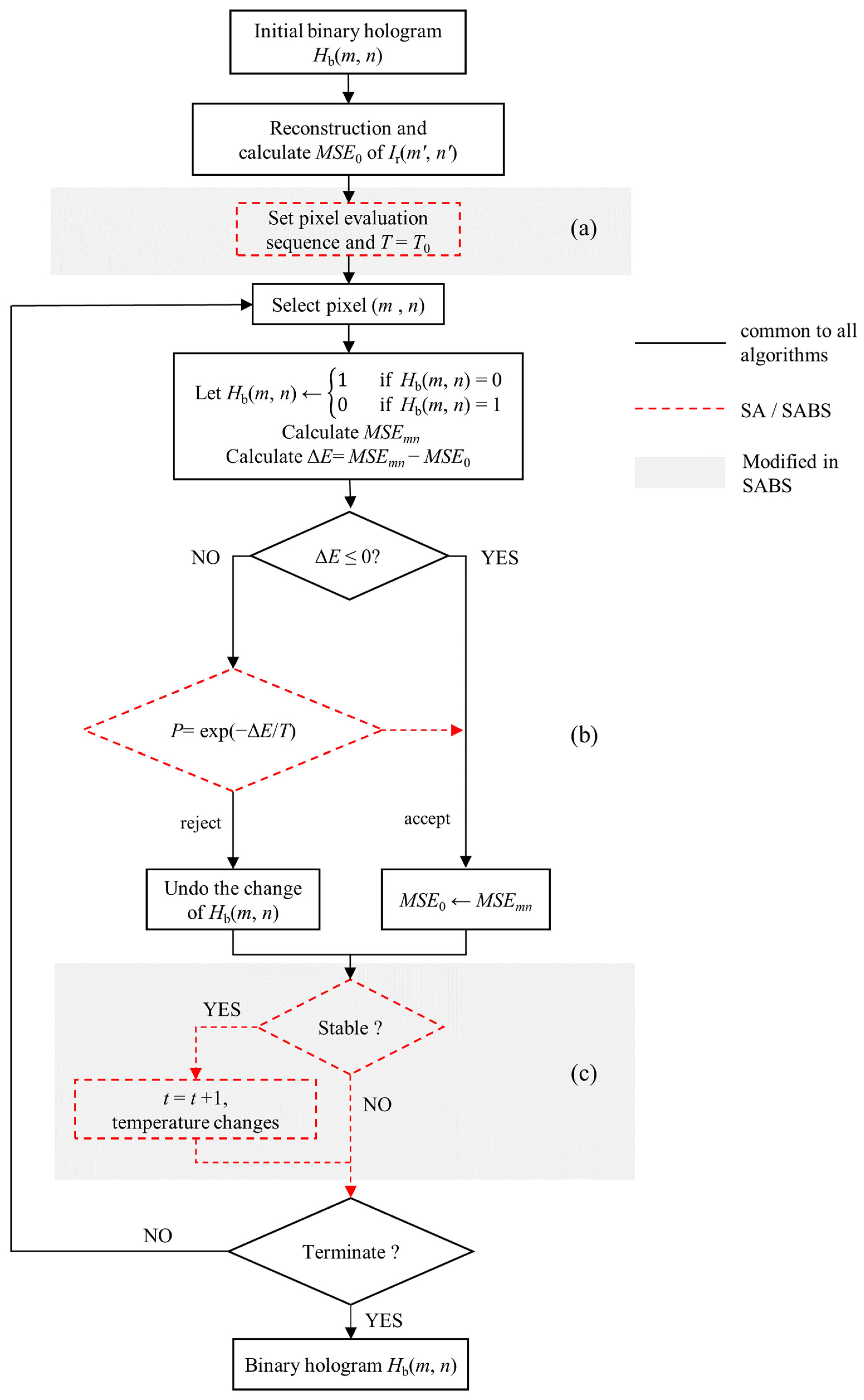
2.1. Direct Binary Search

The flowchart of the DBS is shown in Figure 1, while the steps in red are bypassed. First, an initial binary hologram (typically a binary random function) H b ( m , n ) with size M × N is produced. The variables ( m , n ) are the indices of the hologram pixels. The hologram is then reconstructed by the scalar diffraction formula [33] to obtain the reconstructed field. The mean square error (MSE) of the reconstructed image I r ( m , n ) with size M × N is measured as
M S E = 1 M N m n O ( m , n ) I r ( m , n ) 2 ,
and is regarded as the initial cost function M S E 0 . Here, the variables ( m , n ) are the indices of the reconstructed image, and O ( m , n ) is the target image. In the next step, the hologram pixels are evaluated one by one by a raster-scan order. For every pixel, the pixel value is changed according to
H b ( m , n ) 1 if H b ( m , n ) = 0 0 if H b ( m , n ) = 1 ,
where “ ” means that the value on the left side is replaced by the value on the right side. The updated binary hologram is reconstructed again to measure the MSE ( M S E m n ) of the new reconstructed image. Subsequently, the difference in M S E m n and M S E 0 is calculated by
Δ E = M S E m n M S E 0 .
If Δ E is larger than zero, the change in pixel value is negative and thus the change is undone. Otherwise, the change is accepted, and the cost function M S E 0 is updated by M S E m n . In one round of evaluation, every pixel of the hologram is evaluated once in the same manner. The algorithm terminates after finishing the preset rounds. Usually, after three to five rounds of evaluations, the binary hologram will converge, i.e., nearly all of the pixel values are unchanged in one round of evaluation.

2.2. Simulated Annealing

Simulated annealing (SA) is an optimization algorithm and has been applied to the production of a phase-only Fourier CGH [32]. Here, we applied SA to the production of a Fresnel BCGH. Because the procedures of SA are similar to those of DBS, the flowchart of the SA is also shown in Figure 1. For simplification, here, we only explain the steps that are not involved in the DBS. In step (a), an initial temperature ( T 0 ) is given, which will be used in step (b). In addition, the pixels are not evaluated in the raster-scan order. Instead, the pixels are randomly selected in SA. The pixel-selection sequence is also generated in step (a). The next step is pixel evaluation [(Equation (3)], and the SA also accepts the pixel-value change if Δ E 0 . However, if Δ E > 0 , SA moves to step (b), which will accept the negative pixel-value change according to the probability
P = exp ( Δ E / T ) ,
where T is the current temperature of the status. In step (c), the status of the calculation is evaluated. In the conventional SA, if the Δ E of any pixel is less than the preset value, e.g., 0.05 of the initial Δ E at the same temperature, then the calculation is regarded to be stable, and the temperature decreases according to the annealing function
T = T 0 1 + t ,
where t 0 , 1 , 2 is the count of temperature changes. This step avoids too fast convergence of the calculation, and thus it is possible to find a BCGH with better quality. However, this algorithm never converges on occasion. In the subsection, we will address this issue in detail.

2.3. Stimulated Annealing Binary Search

The SA can directly produce a BCGH. However, we found some shortcomings of SA, and thus its performance is unstable, which also motivated us to propose the SABS method. The flowchart of the proposed simulated annealing binary search (SABS) method is also shown in Figure 1. It is basically the same as SA, except for some modification in steps (a) and (c). In step (a), conventional SA produces a random sequence of pixels for evaluation. In other words, one pixel is probably evaluated several times, but another pixel was probably never evaluated in the whole calculation. For this reason, the sequence is modified to be “pseudo random”: every pixel must be evaluated once in a round of evaluation with a random sequence, and the random sequence of every evaluation round is different.
The second modification is in step (c). The condition of stability in conventional SA depends on the initial Δ E of the first evaluated pixel in that round. If the initial Δ E is very small, it is nearly impossible to satisfy the condition of stability. When this situation occurs, the temperature will be kept high, and the probability for accepting the negative pixel-value change never decreases. An example of this situation is shown in Figure 2 (the detail of the calculation will be explained in the next section). In Figure 2a, the temperature count for SA is frozen at t = 1561 , and the corresponding probability is shown in Figure 2b. The curve of P is plotted using the average of every 1000 pixel-evaluations to clearly show the trajectory. In Figure 2b, it is noted that the probability for SA does not decrease but increases slightly as the temperature has been frozen. The reason for this is that Δ E gradually decreases with the calculation, which results in a slightly increased p [Equation (4)]. Consequently, the hologram always contains pixels with negative pixel values even at the end of the calculation. To avoid the temperature-frozen problem, we made two modifications. First, we directly change the temperature after evaluating q pixels. In addition, we set T = 0 , i.e., P = 0 , at the last round of the evaluation. In other words, the last round of evaluation bypasses the annealing processing (step (b) and (c) in Figure 1) for converging the calculation. Because the method is not the same as the conventional SA, we call the proposed method the simulated-annealing binary search (SABS) method. As a comparison, the t and P (excluded last round) curves of the SABS are also shown in Figure 2a,b, respectively. The problem of being temperature-frozen in the SA was solved in SABS.

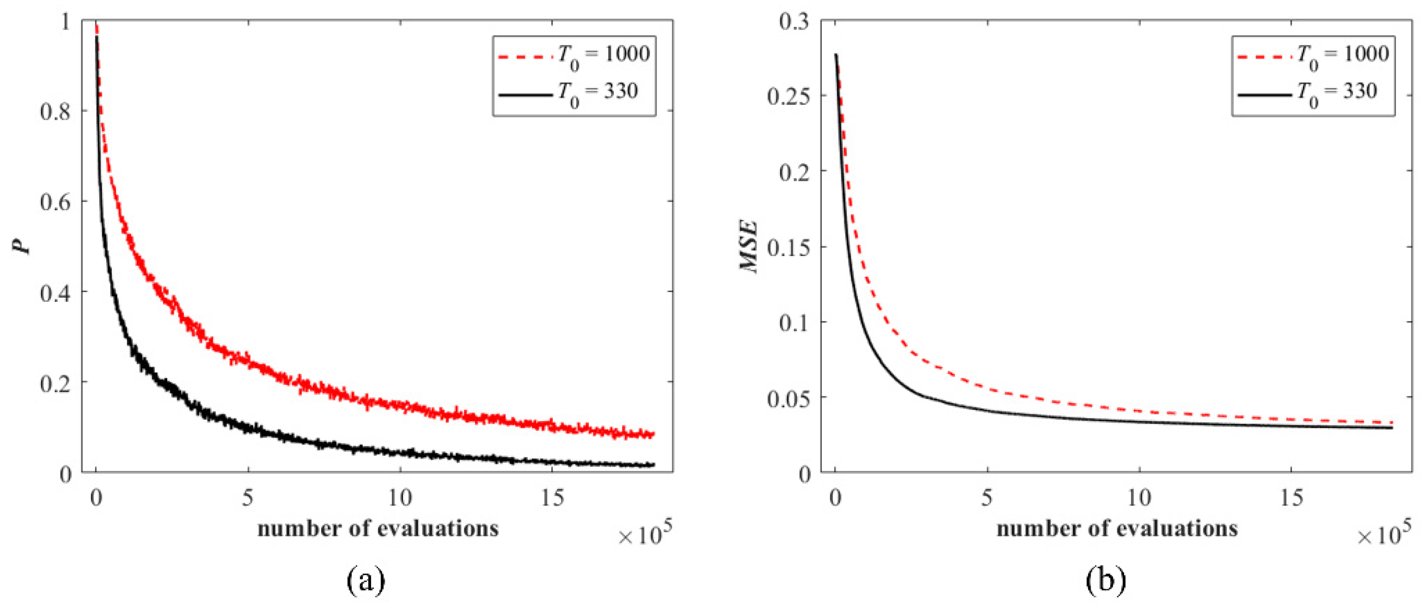
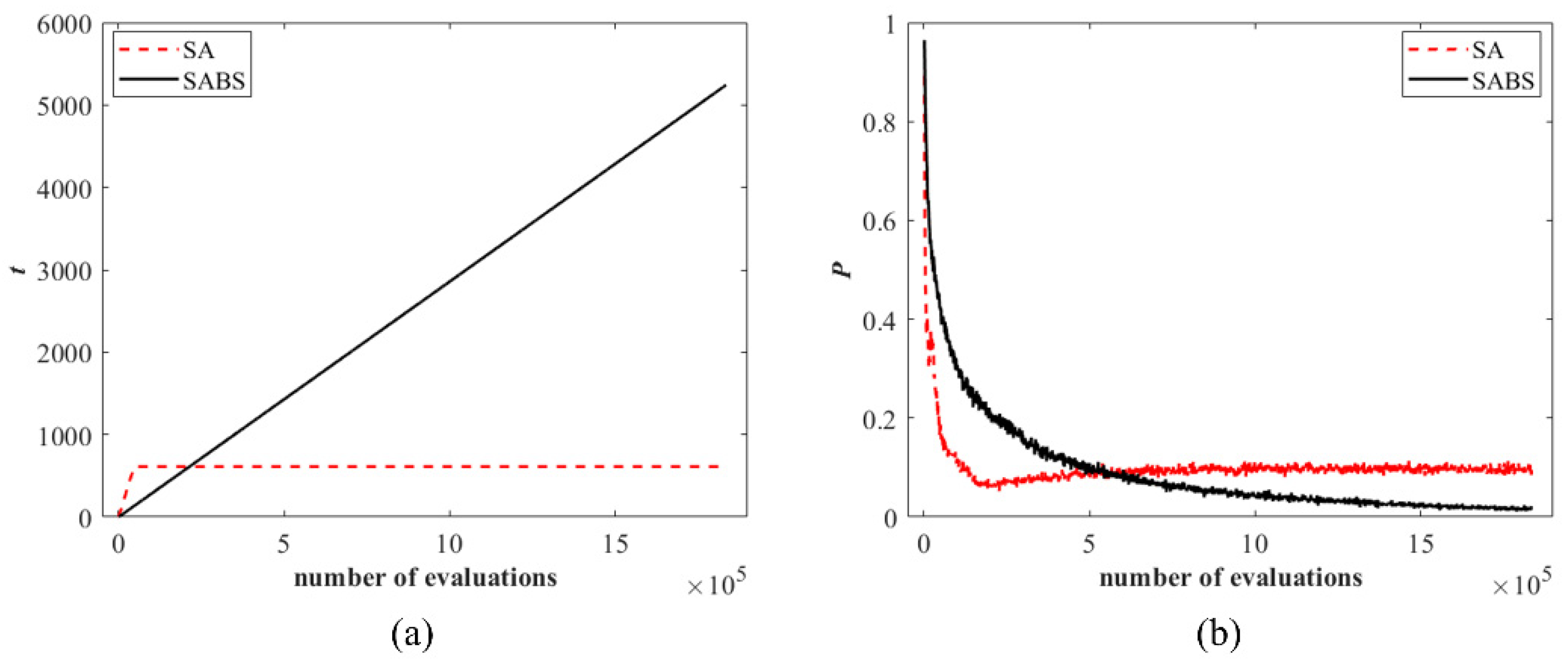
3. Determination of the Parameters in SABS

Although the procedure of SABS was revealed in the last section, the use of SABS is not straightforward because the parameters T 0 and q must be properly set to control the probability P . However, P is a function of Δ E [Equation (4)], which means that the algorithm is sensitive to not only the environmental conditions (wavelength, object distance, etc.), but also the object function. In other words, the parameters must be found by trial and error for every hologram, which is time-consuming and impractical for display applications. For this reason, we developed a methodology to determine the parameters quickly. The discussion comes with some simulations using the following setup. The hologram size, as well as the size of the object (i.e., the target image), is 512 × 512 pixels, with a pixel pitch of 7.6 μ m . The distance between the hologram and the object is 300 mm , and the wavelength is 0.635 μ m . The algorithms can be applied to produce either on-axis holograms or the off-axis holograms. For producing an off-axis hologram, a plane wave with a 1.6 ° off-set angle was applied as the reference light. In the evaluation of every pixel value, the method of look-up table was applied to speed up the computing [30]. The reconstruction of the resulting BCGH was implemented by the angular spectrum method.
To begin with, the number of rounds of evaluations was set according to the tradeoff between the hologram quality and the computing time. In the demonstration, we adopted eight rounds of evaluations, i.e., seven rounds of the modified SA and the last round of binary search. The parameter q is to be determined. It should be noted that the probability [Equations (4) and (5)] is a function of T 0 , Δ E , and t . Therefore, the range of t can be flexible (e.g., t = 0 ~ 6000 ), whereas the probability curve is kept the same by adjusting T 0 . From this point of view, we set q = 350 and the corresponding maximum t is 5243 ( 512 × 512 × 7 / 350 ). Finally, a suitable T 0 was determined. The probability curves for two different T 0 ’s are shown in Figure 3a. The MSE curves corresponding to the two probability curves are shown in Figure 3b. In this example, T 0 = 1000 is not a good choice because its probability curve is still high at the end of the evaluation, which results in a larger MSE. The probability curve can be lowered by using a smaller T 0 for the next trail. As a rule of thumb, the probability at the end of evaluation is better in the range of 0.01~0.02. The curve for T 0 = 333 in Figure 3a is the resulting good probability curve. Usually, the suitable T 0 can be found within some trials.
The above procedure to find the suitable parameters is effective. However, if this procedure must be carried out every time a new hologram is produced, the time cost will be substantial. Fortunately, it is possible to use the same parameters for producing other BCGHs with the same setup. The key point is still the control of the probability, which is a function of Δ E . It is noted that MSE is proportional to the squared intensity of the target image, so as Δ E . This can be expressed as Δ E O ¯ 2 , where O ¯ is the average of the target image. Because Δ E is the numerator in the argument of the probability function [Equation(4)], we can let the denominator be proportional to O ¯ 2 in order to eliminate the influence of different target images. Explicitly, we only need to use a modified initial temperature T ˜ 0 ,
T ˜ 0 = O ¯ 2 O ¯ 0 2 T 0 ,
where O ¯ 0 is the average of the target image for finding the parameter T 0 . In this way, the probability curves corresponding to different target images will be nearly the same.

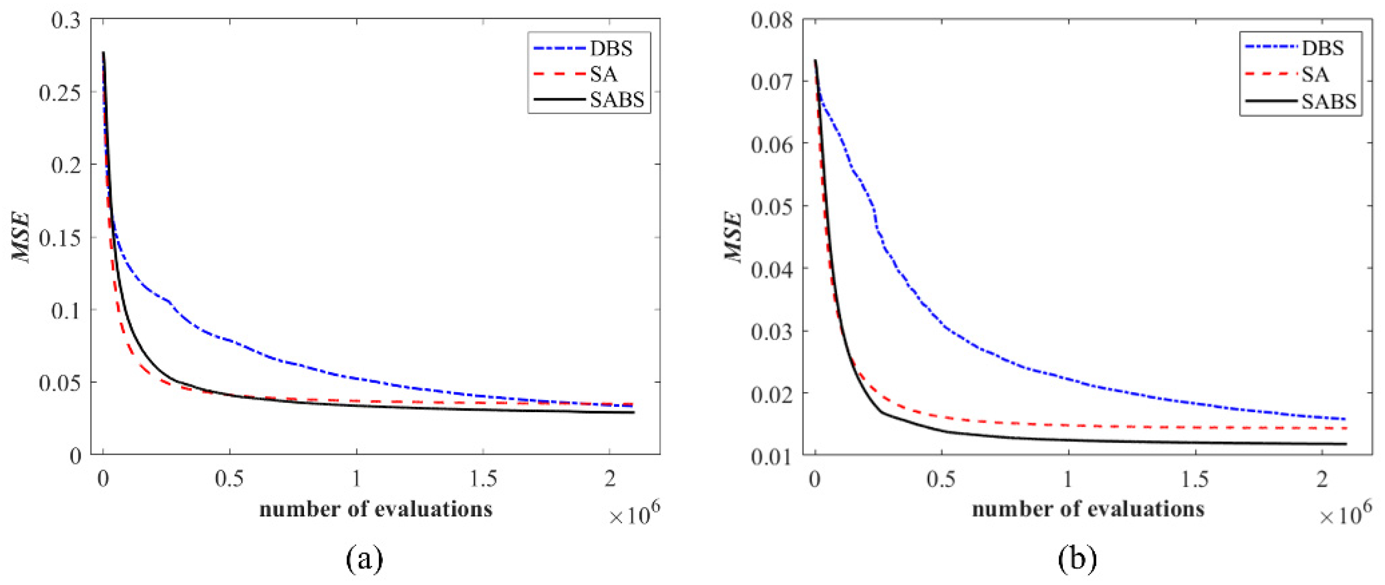
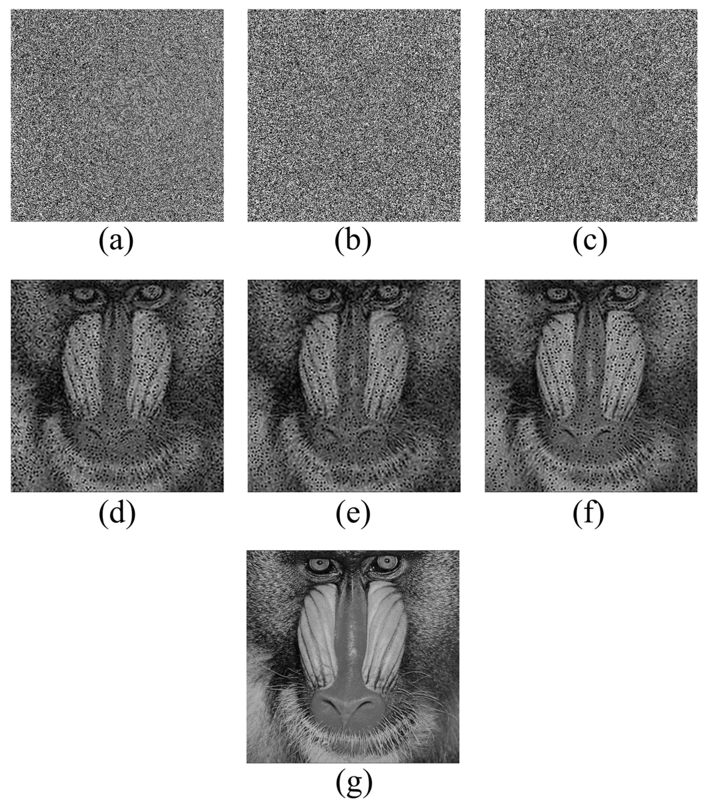
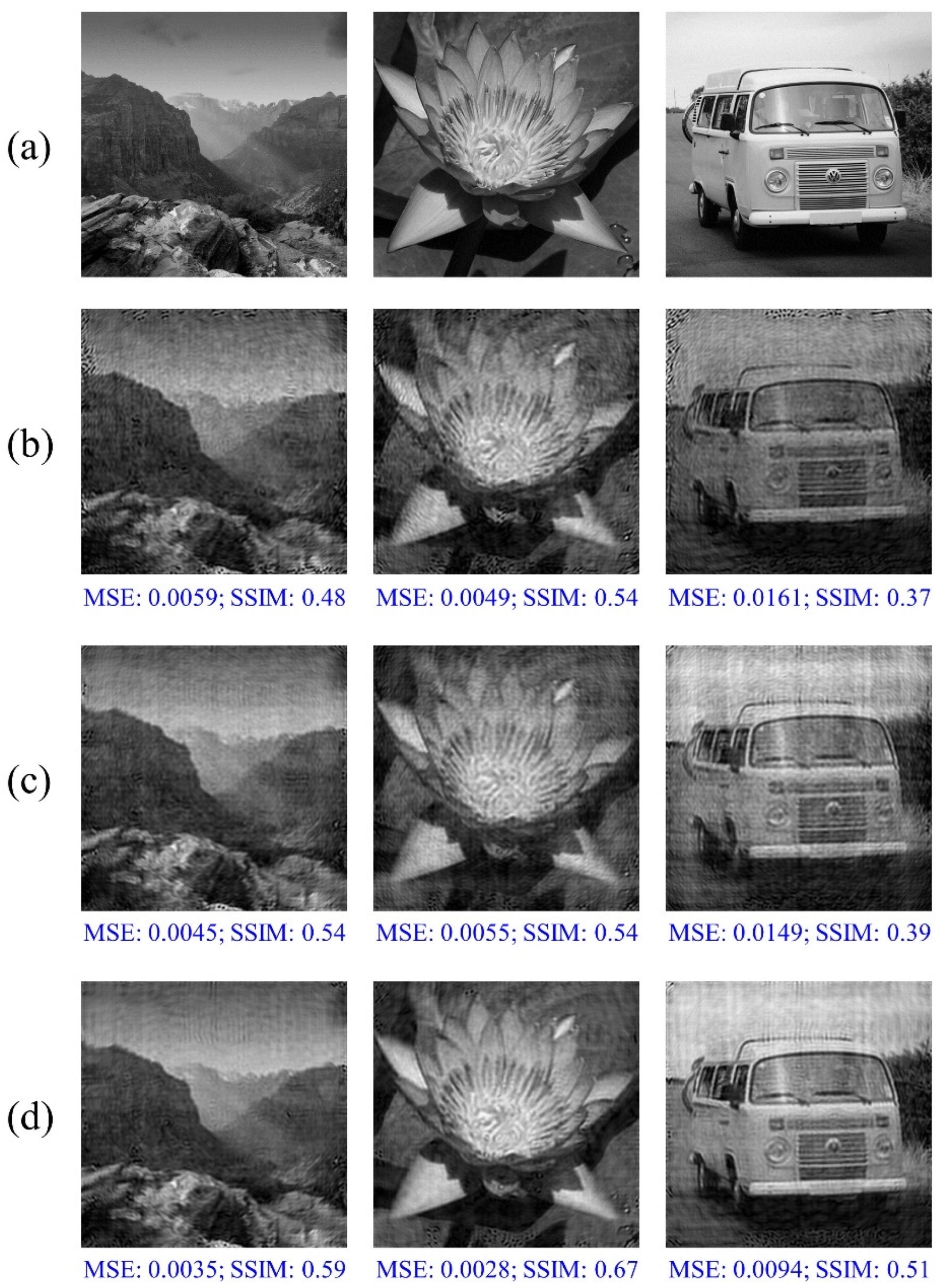
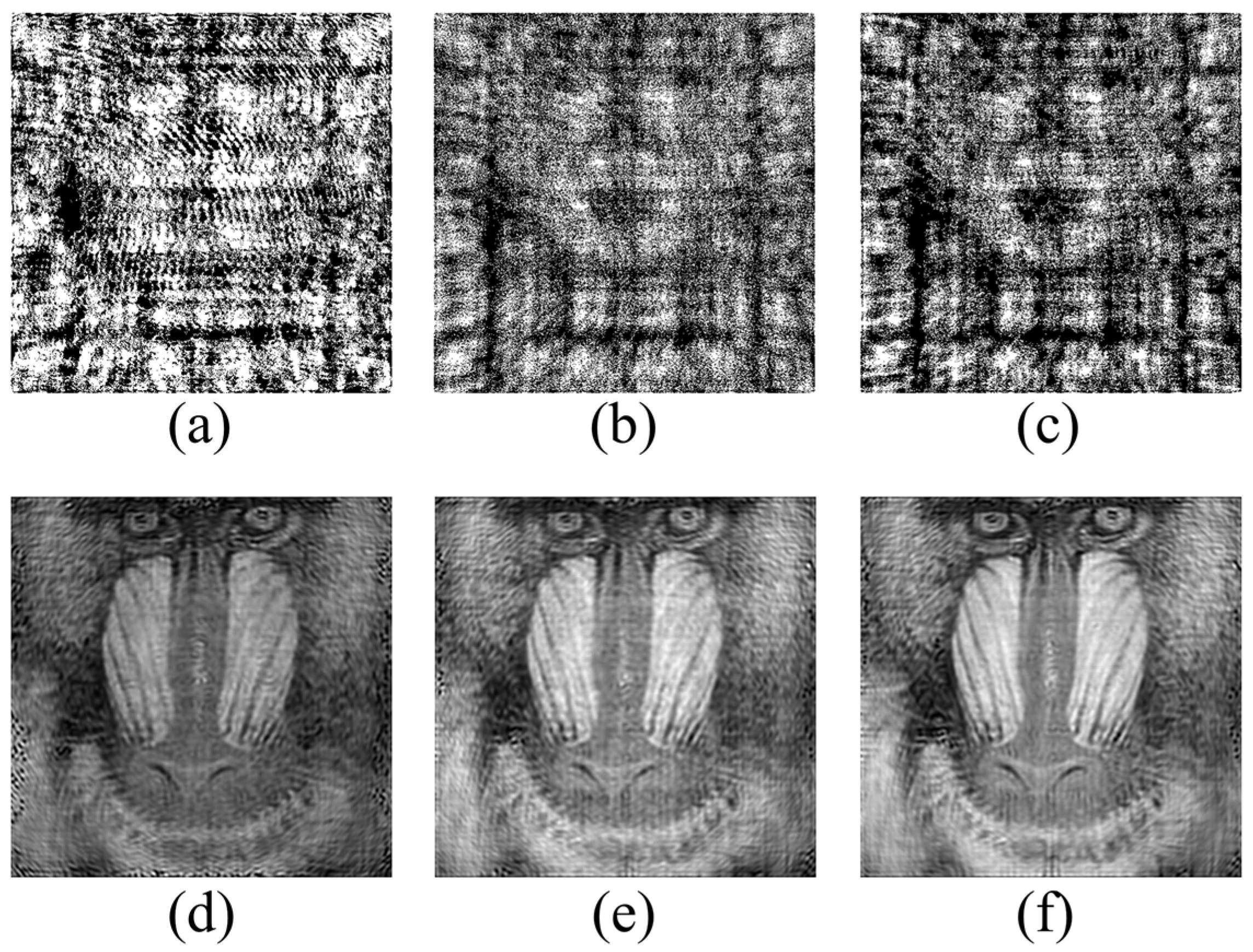
4. Results and Discussions

We compared the performance of the DBS, the SA, and the proposed SABS with both the off-axis scheme and the on-axis scheme, respectively. The MSE curves versus the number of evaluations are shown in Figure 4. The resulting BCGHs and the corresponding reconstructed images are shown in Figure 5 (off-axis) and Figure 6 (on-axis), while the performance metrics, including the MSE, the structural similarity (SSIM) index [34], and the diffraction efficiency, are listed in Table 1. Here, the diffraction efficiency is defined as the ratio of the light energy in the region of interest (ROI) and the total incident light energy. According to the definition, the maximum diffraction efficiency of the BCGHs cannot exceed 50% because the binary-amplitude CGH will typically absorb 50% of the incident light energy.
For the off-axis BCGHs [Figure 4a], the MSE for SA drops quickly in the forepart, but then does not change much. At the end of the evaluation, SA is even worse than that of the DBS. The reason for this is that the conventional SA always retains negative-influence pixels as the temperature is frozen. In contrast, both DBS and SABS can continuously improve the quality up until the end of the evaluations. At the end of the calculation, the quality of the SABS BCGH is the best among the three methods. It should be noted that the diffraction efficiency of the off-axis holograms is low. This is the reason for why the speckle noise is apparent in the reconstructed images (Figure 5d–f). The diffraction efficiency of the DBS BCGH is higher than that of the SA BCGH and the SABS BCGH. It is reasoned that there is a trade-off between the diffraction efficiency and the image quality for the BCGHs. As the SABS focuses on the improvement in the quality, it sacrifices the diffraction efficiency.
For the on-axis BCGHs (Figure 4b), the difference between the three methods is clearer, and the SABS is always better than DBS and SA in all calculation stages. Similarly, the diffraction efficiency of the DBS BCGH is the highest. It is noted that all of the discussed methods are optimization-based algorithms. In the production of the on-axis BCGHs, both the zeroth-order light and the twin image are in the region of interest, and thus are taken into account in the optimization based on the MSE. For this reason, both the image quality and the diffraction efficiency in the on-axis scheme are better than those in the off-axis scheme.
The parameter T 0 was found by using the target image in Figure 5g. By using the modification method in Equation (6), we produced more BCGHs of different target images. The reconstructed images of the BCGHs are shown in Figure 7. The quality of the reconstructed images of SABS BCGHs are also the best, which proves the ability of the control of the probability curve.

5. Conclusions

In this paper, we have proposed and investigated the simulated-annealing binary search (SABS) for the production of binary computer-generated holograms. Being similar to the simulated annealing (SA), SABS allows for negative pixel-value changes in the early stage of the calculation. This enables SABS to find a better solution than DBS. On the other hand, SABS uses a fixed temperature change rate, which avoids the problem of being temperature-frozen in SA. Finally, SABS bypasses the step of accepting negative pixel-value changes in the last round of the evaluation, which minimizes the error of the produced BCGHs. The determination of the initial temperature is a time-consuming procedure. We have also proven that, as an ideal initial temperature has been found from a target image, the initial temperatures for other target images can be easily found without additional simulation trials. On average, the MSE of the SABS holograms decreases by 38% and 32%, respectively, in comparison with the DBS holograms and the SA holograms. It should be noted that the number of evaluation rounds is large in our simulation, and thus the calculation of all methods converges. For a smaller number of evaluation rounds, the difference between DBS and SABS should be larger, as shown in Figure 4b. The only shortcoming of the SABS BCGHs is that its diffraction efficiency is lower than that of the DBS BCGHs, which is believed to be the cost in achieving the extremely low MSE. Finally, we only discussed the production of binary-amplitude CGHs in this paper. According to our preliminary study, the SABS can be also applied to produce binary-phase CGHs. This will be investigated in the future.

Author Contributions

Conceptualization, J.-P.L. and C.-M.T.; methodology, C.-M.T.; investigation, C.-M.T.; writing—original draft preparation, J.-P.L.; project administration, J.-P.L.; funding acquisition, J.-P.L. All authors have read and agreed to the published version of the manuscript.

Funding

This research was funded by Ministry of Science and Technology of Taiwan (MOST), grant number 109-2221-E-035-076-MY3.

Data Availability Statement

Not applicable.

Conflicts of Interest

The authors declare no conflict of interest.

References

  1. Poon, T.-C. (Ed.) Digital Holography and Three-Dimensional Display; Springer: Berlin, Germany, 2006. [Google Scholar]
  2. He, Z.; Sui, X.; Jin, G.; Chu, D.; Cao, L. Optimal quantization for amplitude and phase in computer-generated holography. Opt. Express 2021, 29, 119–133. [Google Scholar] [CrossRef] [PubMed]
  3. Zhang, H.; Zhao, Y.; Cao, L.; Jin, G. Layered holographic stereogram based on inverse Fresnel diffraction. Appl. Opt. 2016, 55, A154–A159. [Google Scholar] [CrossRef] [PubMed]
  4. Zhang, Z.; Liu, J.; Gao, Q.; Duan, X.; Shi, X. A full-color compact 3D see-through near-eye display system based on complex amplitude modulation. Opt. Express 2019, 27, 7023–7035. [Google Scholar] [CrossRef] [PubMed]
  5. Park, M.-C.; Lee, B.-R.; Son, J.-Y.; Chernyshov, O. Properties of DMDs for holographic displays. J. Mod. Opt. 2015, 62, 1600–1607. [Google Scholar] [CrossRef]
  6. Takaki, Y.; Yokouchi, M. Speckle-free and grayscale hologram reconstruction using time-multiplexing technique. Opt. Express 2011, 19, 7567–7579. [Google Scholar] [CrossRef]
  7. Mori, Y.; Fukuoka, T.; Nomura, T. Speckle reduction in holographic projection by random pixel separation with time multiplexing. Appl. Opt. 2014, 53, 8182–8188. [Google Scholar] [CrossRef]
  8. Lee, B.; Yoo, D.; Jeong, J.; Lee, S.; Lee, D.; Lee, B. Wide-angle speckleless DMD holographic display using structured illumination with temporal multiplexing. Opt. Lett. 2020, 45, 2148–2151. [Google Scholar] [CrossRef]
  9. Sando, Y.; Barada, D.; Yatagai, T. Full-color holographic 3D display with horizontal full viewing zone by spatiotemporal-division multiplexing. Appl. Opt. 2018, 57, 7622–7626. [Google Scholar] [CrossRef]
  10. Takahashi, T.; Shimobaba, T.; Kakue, T.; Ito, T. Time-Division Color Holographic Projection in Large Size Using a Digital Micromirror Device. Appl. Sci. 2021, 11, 6277. [Google Scholar] [CrossRef]
  11. Takaki, Y.; Matsumoto, Y.; Nakajima, T. Color image generation for screen-scanning holographic display. Opt. Express 2015, 23, 26986–26998. [Google Scholar] [CrossRef]
  12. Li, J.; Smithwick, Q.; Chu, D. Full bandwidth dynamic coarse integral holographic displays with large field of view using a large resonant scanner and a galvanometer scanner. Opt. Express 2018, 26, 17459–17476. [Google Scholar] [CrossRef] [PubMed]
  13. Chlipala, M.; Kozacki, T. Color LED DMD holographic display with high resolution across large depth. Opt. Lett. 2019, 44, 4255–4258. [Google Scholar] [CrossRef] [PubMed]
  14. Masuda, K.; Saita, Y.; Toritani, R.; Xia, P.; Nitta, K.; Matoba, O. Improvement of Image Quality of 3D Displayby Using Optimized Binary Phase Modulation and Intensity Accumulation. J. Disp. Technol. 2016, 12, 472–477. [Google Scholar] [CrossRef]
  15. Liu, J.-P.; Wu, M.-H.; Tsang, P.W.M. 3D display by binary computer-generated holograms with localized random down-sampling and adaptive intensity accumulation. Opt. Express 2020, 28, 24526–24537. [Google Scholar] [CrossRef]
  16. Liu, J.-P.; Lin, Y.-C.; Jiao, S.; Poon, T.-C. Performance Estimation of Intensity Accumulation Display by Computer-Generated Holograms. Appl. Sci. 2021, 11, 7729. [Google Scholar] [CrossRef]
  17. Cheung, W.K.; Tsang, P.; Poon, T.-C.; Zhou, C. Enhanced method for the generation of binary Fresnel holograms based on grid-cross downsampling. Chin. Opt. Lett. 2011, 9, 120005. [Google Scholar] [CrossRef]
  18. Tsang, P.; Poon, T.-C.; Cheung, W.K.; Liu, J.-P. Computer generation of binary Fresnel holography. Appl. Opt. 2011, 50, B88–B95. [Google Scholar] [CrossRef]
  19. Tsang, P.; Cheung, W.K.; Poon, T.-C.; Liu, J.-P. An enhanced method for generation of binary Fresnel hologram based on adaptive and uniform grid-cross down-sampling. Opt. Commun. 2012, 285, 4027–4032. [Google Scholar] [CrossRef]
  20. Tsang, P.W.M.; Poon, T.-C.; Jiao, A.S.M. Embedding intensity image in grid-cross down-sampling (GCD) binary holograms based on block truncation coding. Opt. Commun. 2013, 304, 62–70. [Google Scholar] [CrossRef]
  21. Yang, G.; Jiao, S.; Liu, J.-P.; Lei, T.; Yuan, X. Error diffusion method with optimized weighting coefficients for binary hologram generation. Appl. Opt. 2019, 58, 5547–5555. [Google Scholar] [CrossRef]
  22. Jiao, S.; Zhang, D.; Zhang, C.; Gao, Y.; Lei, T.; Yuan, X. Complex-Amplitude Holographic Projection With a Digital Micromirror Device (DMD) and Error Diffusion Algorithm. IEEE J. Sel. Top. Quantum Electron. 2020, 26, 1–8. [Google Scholar] [CrossRef]
  23. Min, K.; Park, J.-H. Quality enhancement of binary-encoded amplitude holograms by using error diffusion. Opt. Express 2020, 28, 38140–38154. [Google Scholar] [CrossRef] [PubMed]
  24. Cheremkhin, P.A.; Kurbatova, E.A.; Evtikhiev, N.N.; Krasnov, V.V.; Rodin, V.G.; Starikov, R.S. Comparative analysis of off-axis digital hologram binarization by error diffusion. J. Opt. 2021, 23, 075703. [Google Scholar] [CrossRef]
  25. Wyrowski, F.; BryngdahI, O. Iterative Fourier-transform algorithm applied to computer holography. J. Opt. Soc. Am. A 1988, 5, 1058–1965. [Google Scholar] [CrossRef]
  26. Wu, C.-H.; Chen, C.-L.; Fiddy, M.A. Iterative procedure for improved computer-generated-hologram reconstruction. Appl. Opt. 1993, 32, 5135–5140. [Google Scholar] [CrossRef] [PubMed]
  27. Piestun, R.; Spektor, B.; Shamir, J. On-axis binary-amplitude computer generated holograms. Opt. Commun. 1997, 136, 85–92. [Google Scholar] [CrossRef]
  28. Seldowitz, M.A.; Allebach, J.P.; Sweeney, D.W. Synthesis of digital holograms by direct binary search. Appl. Opt. 1987, 26, 2788–2798. [Google Scholar] [CrossRef]
  29. Jennison, B.K.; Allebach, J.P.; Sweeney, D.W. Efficient design of direct-binary-search computer-generated holograms. J. Opt. Soc. Am. A 1991, 8, 652–660. [Google Scholar] [CrossRef]
  30. Liu, J.-P.; Yu, C.-Q.; Tsang, P.W.M. Enhanced direct binary search algorithm for binary computer-generated Fresnel holograms. Appl. Opt. 2019, 58, 3735–3741. [Google Scholar] [CrossRef]
  31. Cheremkhin, P.A.; Evtikhiev, N.N.; Krasnov, V.V.; Starikov, R.S.; Zlokazov, E.Y. Iterative synthesis of binary inline Fresnel holograms for high-quality reconstruction in divergent beams with DMD. Opt. Lasers Eng. 2022, 150, 106859. [Google Scholar] [CrossRef]
  32. Yoshikawa, N.; Yatagai, T. Phase optimization of a kinoform by simulated annealing. Appl. Opt. 1994, 33, 863–868. [Google Scholar] [CrossRef] [PubMed]
  33. Liu, J.-P. Controlling the aliasing by zero-padding in the digital calculation of the scalar diffraction. J. Opt. Soc. Am. A 2012, 29, 1956–1964. [Google Scholar] [CrossRef] [PubMed]
  34. Wang, Z.; Bovik, A.C.; Sheikh, H.R.; Simoncelli, E.P. Image Quality Assessment: From Error Visibility to Structural Similarity. IEEE Trans. Image Process. 2004, 13, 600–612. [Google Scholar] [CrossRef] [PubMed]
Figure 1. Flowchart of direct binary search (DBS), simulated annealing (SA), and simulated annealing binary search (SABS).
Photonics 09 00581 g001
Figure 2. The comparison between SA and SABS. (a) The count of temperature change versus the number of evaluations. (b) The probability versus the number of evaluations.
Photonics 09 00581 g002
Figure 3. The SABS using different T 0 . (a) The probability versus the number of evaluations. (b) The MSE versus the number of evaluations.
Photonics 09 00581 g003
Figure 4. The comparison with DBS, SA, and SABS. (a) The MSE versus the number of evaluations for the off-axis scheme. (b) The MSE versus the number of evaluations for the off-axis scheme.
Photonics 09 00581 g004
Figure 5. Off-axis BCGHs and the reconstructed images. The BCGHs are produced by DBS (a), SA (b), and SABS (c), respectively. Their reconstructed images are in (d), (e), and (f), respectively. (g) is the target image.
Photonics 09 00581 g005
Figure 6. On-axis BCGHs and the reconstructed images. The BCGHs are produced by DBS (a), SA (b), and SABS (c), respectively. Their reconstructed images are in (d), (e), and (f), respectively.
Photonics 09 00581 g006
Figure 7. Reconstructed images of three different target images. (a) The target images. (obtained from Pixabay) (b) The reconstructed images of DBS BCGHs. (c) The reconstructed images of SA BCGHs. (d) The reconstructed images of SABS BCGHs.
Photonics 09 00581 g007
Table 1. Performances of different BCGH methods.
MetricsDBSSASABS
off-axis BCGHMSE0.03340.03490.0290
SSIM0.2220.2090.246
diffraction efficiency3.51%1.34%1.73%
on-axis BCGHMSE0.01580.01440.0118
SSIM0.3290.3340.380
diffraction efficiency32.2%19.9%17.8%
Publisher’s Note: MDPI stays neutral with regard to jurisdictional claims in published maps and institutional affiliations.

