Novel Measurement-Based Efficient Computational Approach to Modeling Optical Power Transmission in Step-Index Polymer Optical Fiber

Abstract

Polymer optical fibers (POFs) are playing an important role in industrial applications nowadays due to their ease of handling and resilience to bending and environmental effects. A POF can tolerate a bending radius of less than 20 mm, it can work in environments with temperatures ranging from −55 °C to +105 °C, and its lifetime is around 20 years. In this paper, we propose a novel, rigorous, and efficient computational model to estimate the most important parameters that determine the characteristics of light propagation through a step-index polymer optical fiber (SI-POF). The model uses attenuation, diffusion, and mode group delay as functions of the propagation angle to characterize the optical power transmission in the SI-POF. Taking into consideration the mode group delay allows us to generalize the computational model to be applicable to POFs with different index profiles. In particular, we use experimental measurements of spatial distributions and frequency responses to derive accurate parameters for our SI-POF simulation model. The experimental data were measured at different fiber lengths according to the cut-back method. This method consists of taking several measurements such as frequency responses, angular intensity distributions, and optical power measurements over a long length of fiber (>100 m), then cutting back the fiber while maintaining the same launching conditions and repeating the measurements on the shorter lengths of fiber. The model derivation uses an objective function to minimize the differences between the experimental measurements and the simulated results. The use of the matrix exponential method (MEM) to implement the SI-POF model results in a computationally efficient model that is suitable for POF-based system-level studies. The efficiency gain is due to the independence of the calculation time with respect to the fiber length, in contrast to the classic analytical solutions of the time-dependent power flow equation. The robustness of the proposed model is validated by calculating the goodness-of-fit of the model predictions relative to experimental data.

1. Introduction

Plastic optical fiber (POF) frequently uses polymethyl methacrylate (PMMA) as core material and fluorinated PMMA as a cladding material. Apart from advantages shared with glass optical fibers such as their lightweight and electromagnetic interference (EMI) immunity, PMMA POFs have large numerical apertures (0.5) and sizes (1 mm diameter). Usually, 96% or more of the cross section is the core. This enhances the transmission characteristic of the POFs and the tolerable variability of lateral connector misalignment and other localized disturbances such as bends [1,2,3].

POFs are currently widely used in industry due to their physical and design characteristics that make the installation and maintenance process more efficient, positively impacting its total cost. The main applications of POFs are in data networks and sensors. The data networks applications are focused primarily on domestic networks [4,5], vehicular networks [6], avionics platforms [7], and industrial controls and automation (ProfiBus, ProfiNet, and industrial Ethernet over POF [8]). The sensors applications [9,10,11,12,13,14] use mainly three common methods for measuring, intensity modulation, phase modulation, and Bragg wavelength shift, and take advantage of POFs’ high fracture toughness, high flexibility in bending, high sensitivity to strain, and potential negative thermo-optic coefficients.

According to their index profiles, there are two types of POFs. The first one is the step-index (SI) POF, which has the same refractive index throughout the core. The second one is the graded-index (GI) POF in which the refractive index gradually changes from the center of the core through the junction of the core and the cladding, reducing its large modal dispersion [15]. The SI-POF is the most used type in different industrial applications and has its lowest losses at 520 nm (green), 560 nm (yellow), and 650 nm (red). Its bandwidth at 50 m is approximately 100 MHz, but multi-gigabit rates are possible when using spectral efficiency modulation techniques [16,17]. In the last decades, polyperfluoro-butenylvinylether materials, commercially known as CYTOP, have played a relevant role in the manufacturing of POFs. This polymer has allowed SI-POFs to overcome their limitations, showing a low attenuation in the infrared spectrum (~10 dB/km), and supporting transmission rates up to 10 Gbit/s for fiber length of 100 m [18].

In the case of PMMA POF, its tight power budget and its limited capacity motivate the need for a flexible and dynamic system-level simulation framework. This will allow testing of different layouts and scenarios before the deployment of POF links in order to evaluate the entire system performance. However, the traditional methods for the solution of Gloge’s power flow equation have proved to require a large computational time [19,20,21] due to their dependence on the fiber length. The time consumed by calculations plays a relevant role in longer fiber lengths. Mateo et al. [22] proposed an approach based on a recurrent matrix equation to model POF and passive components such as connectors [23]. In this approach, light propagation throughout the fiber is modeled by a matrix that is calculated from the fiber’s characteristic functions. These functions are different for each fiber type. However, this method shows the same limitations as the traditional methods for longer fiber lengths. Stepniak et al. proposed a method to solve Gloge’s power equation based on the matrix exponential [24]. The main advantage is that its computational calculations do not depend on the fiber length. Therefore, this method is computationally efficient for longer fiber lengths.

Taking into consideration the drawbacks and advantages of the previous methods in order to develop a flexible and accurate simulation framework, the present article proposes a computational algorithm to estimate the fiber characteristic functions, i.e., diffusion, attenuation, and mode group delay, as functions of the propagation angle. These functions are obtained from experimental measurements, intensity distributions and frequency responses, which are obtained for different fiber lengths. The novelty of this approach in comparison to previous methods [22,25] is trifold. Firstly, we combine measurements in both the spatial and frequency domains to estimate the fiber characteristic functions. Secondly, we incorporate the mode group delay function to model fibers with different index profiles. Thirdly, we solve the power propagation differential equation using the matrix exponential method (MEM), which provides a more computationally efficient implementation [24]. The fiber characteristic functions are described as functions of the propagation angle using a set of estimated parameters to minimize the differences between the experimental measurements and the simulated results.

This article is organized as follows: Firstly, Section 2 contains a description of the fiber types used in the experiment and the protocol to obtain the received or output optical powers, S₂₁ transmission parameters, and far field pattern (FFP) images. Secondly, Section 3 contains a mathematical explanation of the proposed computational algorithm. Thirdly, Section 4 contains a detailed description and analysis of the results obtained in Section 2. Finally, Section 5 contains the conclusions.

2. Materials and Methods

The present section contains an explanation of the fiber types, experimental setup, and experimental methodology. The described procedures allow us to obtain the intensity distributions as a function of the angle at the fiber output from the measurements of FFP images, the frequency responses from the measurements of the S₂₁ transmission parameter, and the received optical power. The cut-back method [26] is used as a measuring technique to ensure that all the measurements as a function of the fiber length are kept under the same launching conditions. This methodology has been thoroughly described by Losada et al. [27]. This section only provides a summary of it.

2.1. Fiber Types and Experimental Setup

The two PMMA SI-POFs used in the experiment were of 1 mm core diameter with different numerical apertures (NAs) to test the ability of the model to describe their different results. They were both manufactured by Mitsubishi Chemical Company. The first one was BH4001 [28], which is a simplex fiber with a NA of 0.58 and a core refractive index of 1.49. This fiber is also called Eska Simplex High-Performance Plastic Optical Fiber Cable, and it is used at temperatures up to 105 °C in industrial data applications. The second one was MH4001 [29], which is a simplex fiber with a NA of 0.3 and a core refractive index of 1.49. This fiber is also called Eska Mega High-Performance Plastic Optical Fiber Cable, and due to its reduced aperture, it is used for high bandwidth applications. The reduced aperture is achieved by a double-cladding structure [1].

Figure 1 depicts the experimental setup. This system was subdivided into three subsystems to acquire the optical power, the FFP images, and the S₂₁ transmission parameters shown in Figure 1a, 1b, and 1c respectively. First and foremost, the fiber input end was connected to the laser diode source using a straight tip (ST) connector. It remained in this position throughout the whole experiment to guarantee that all fiber lengths were tested under the same launching conditions. The fiber output end was connected to a specific device depending on the measurement that was acquired according to the subsystems shown in Figure 1a–c.

The optical source was a laser diode (L520P50) that emits light at 520 nm and it was mounted in a LDM9T, both from Thorlabs. The current bias of the laser was set at 80 mA by a laser diode controller LDC205 from Thorlabs as well. The green light was selected for the experiments because the PMMA POFs have lower attenuation at the 520 nm region of the spectrum than in the red wavelength region. Therefore, we were able to measure longer fiber lengths. Moreover, it was shown that the changes in fiber frequency response with wavelength are small and lower than fiber variability [27].

Figure 1a depicts the method to acquire the optical power independently of the subsystems (b) and (c). It used the power meter PM100USB equipped with a sensor S150C. Both were manufactured by Thorlabs.

Figure 1b depicts the method to acquire the FFP images that are reflected on a white screen placed in front of the fiber output end [22]. The fiber end was inserted into a VersaLink (VL) connector and placed on a pedestal at 7.5 cm from the white screen. The reflected images on the white screen were captured by a 12 bit monochrome cooled digital camera QICAM FAST 1394 manufactured by QImaging. The whole procedure was computer controlled.

Figure 1c depicts the method used to acquire measurements of the S₂₁ transmission parameter. The laser diode mount LDM9T had a radio frequency (RF) input for modulating the laser diode L520P50 with an external RF source. The experiment used the RF output of a vector network analyzer (VNA) E5071C from Agilent to drive the RF input of the laser source. The fiber output end was connected to a silicon PIN photodetector SPD-2 manufactured by Graviton with a nominal bandwidth of 1.2 GHz. The RF output of the photodetector was connected to the VNA to acquire the S₂₁ transmission parameter.

2.2. Experimental Methodology

The experimental methodology was formulated on the application of the cut-back method [26]. This method is well-known in the industry, and it consists of comparing the optical power transmitted or another magnitude through varying lengths of longer spans of fiber to a reference short span of fiber. The process started with a long fiber length. We measured the FFP images, S₂₁ transmission parameter, and received optical power. All these measurements were taken several times calculating their average and their standard deviation. After all the measurements were collected, we proceeded to cut-back the initial long fiber length from the fiber output end. After this, the measurement protocol started again.

The two different types of fibers were reeled over 20 cm spools and they were subjected to the same measurement protocol. The starting fiber length for the BH4001 fiber was 100 m, and the MH4001 fiber was 150 m. In the case of the BH4001 fiber, the measurements were taken considering fiber lengths of 1, 5, 10, 15, 20, 30, 40, 50, 60, 70, 85, and 100 m. In the case of the MH4001 fiber, the fiber lengths were 1, 3, 10, 15, 20, 30, 40, 50, 60, 70, 85, 100, 110, 130, and 150 m.

The radial profile extracted from the FFP images is equivalent to the angular intensity distribution at the fiber output [22]. These profiles were a function of the propagation angle for our experimental conditions, and they had 260 data points in the range of 0° to 45°. The frequency response was obtained from two measurements of the S₂₁ parameter. The first one used a long fiber segment (such as those obtained from the cut-back experiment). The second one used the last measurement of the cut-back experiment (1 m in both fibers). This last S₂₁ measurement was used as a reference and represented the degradation introduced by the optoelectronic devices (transmitter/receiver) as the effects of the fiber can be neglected in the shortest fiber measurements [30]. The frequency response measurements had 1601 data points in the range of 4.5 GHz. These were the maximum quantity of data points and frequency span allowed by the VNA used in the experiment. However, it was limited to a maximum value of ~1.18 GHz, which was suitable for the limits imposed by optoelectronic devices. In order to improve the computational time, the data of the BH4001 and MH4001 fibers were subsampled and limited, as is explained in more detail in Section 3.

3. Computational Model and Fitting Algorithm

This section contains the explanation of the computation algorithm. We propose to estimate the fiber characteristic functions by fitting some of their parameters to experimental measurements. The first part describes the propagation model based on the resolution of the differential power equation using the MEM approach. The second part defines the fiber characteristic functions, i.e., the diffusion, differential mode attenuation, and mode group delay that depend on the propagation angle. These functions vary for different fiber types. Additionally in this subsection, we propose a cost function to obtain the parameters of the characteristic functions from the experimental measurements using an optimization algorithm.

3.1. Computational Model

Gloge’s power flow equation [19,31] is the starting point to develop the computational algorithm proposed in the present paper, and it is given by:

$$\frac{\partial p\left(\theta ,z,t\right)}{\partial z}+\frac{\partial t}{\partial z}\frac{\partial p\left(\theta ,z,t\right)}{\partial t}=-\alpha \left(\theta \right)p\left(\theta ,z,t\right)+\frac{1}{\theta }\frac{\partial }{\partial \theta }\left[\theta D\left(\theta \right)\frac{\partial p\left(\theta ,z,t\right)}{\partial \theta }\right],$$

(1)

where $p\left(\theta ,z,t\right)$ is the optical intensity distribution that describes the power at each propagation angle (mode) at distance $z$ and time $t$; $\theta$ is the propagation angle; $\alpha \left(\theta \right)$ is the differential mode attenuation; and $D\left(\theta \right)$ is the mode coupling or diffusion function. The derivative $\partial t/\partial z$ is the inverse of the group velocity of a mode with propagation angle $\theta$. It is related to the material speed of light, $c/n_{core}$, multiplied by a function to account for the increased path length depending on the propagation angle [31] and it is termed the mode group delay function:

$$\tau \left(\theta \right)=\frac{\partial t}{\partial z}.$$

(2)

Applying the Fourier transform in Equation (1) to work in the frequency domain, and substituting Equation (2) into Equation (1) leads to Equation (3):

$$\frac{\partial P\left(\theta ,z,\omega \right)}{\partial z}=\left[-\alpha \left(\theta \right)-j\omega \tau \left(\theta \right)\right]P\left(\theta ,z,\omega \right)+\frac{1}{\theta }\frac{\partial }{\partial \theta }\left[\theta D\left(\theta \right)\frac{\partial P\left(\theta ,z,\omega \right)}{\partial \theta }\right],$$

(3)

where $P\left(\theta ,z,t\right)$ is the Fourier transform of $p\left(\theta ,z,t\right)$ and both functions contain all the necessary information to obtain the fiber transmission parameters such as the total optical power and bandwidth for a given length.

There are a few analytical approaches to solve differential Equation (3) [31,32]. The standard procedure is based on converting the power flow equation into a recurrent equation and using different methods to reduce computation time [20,22,33,34]. However, these methods share the same drawback. They require more computational time for longer fiber lengths because the calculations are performed iteratively, i.e., the data obtained for the distance $z$ are used to calculate the data at the distance $z+\mathit{\Delta }z$. In addition, the calculation step, $\mathit{\Delta }z$, should not exceed a certain value, otherwise, the solution may not converge [20]. In the case of the MEM proposed by Stepniak, the power flow equation is represented and solved using matrix formalism [24]. Since in MEM the computation time is independent of the fiber length, this approach is computationally more efficient than the standard methods, and it does not have convergence issues.

Expressing Equation (3) in its matrix form leads us to Equation (4):

$$\frac{d{\mathbb{P}}_{\omega }\left(z\right)}{dz}=\left({\mathbb{G}}_{\omega }+ℍ\right){\mathbb{P}}_{\omega }\left(z\right),$$

(4)

where ${\mathbb{P}}_{\omega }\left(z\right)$ is the Fourier transform of the optical intensity distribution $p\left(\theta ,z,t\right)$ in vector form relative to the angular coordinate. It is given by:

$${\mathbb{P}}_{\omega }\left(z\right)={\left[P\left({\theta }_1,z,\omega \right), P\left({\theta }_2,z,\omega \right), \dots ,P\left({\theta }_M,z,\omega \right), \right]}^T,$$

(5)

while ${\mathbb{G}}_{\omega }$ is the diagonal matrix that introduces the effects of differential mode attenuation, and it is independent of the fiber length $z$. However, it depends on frequency ω. Its complex elements are given by:

$${\mathbb{G}}_{m,m}=-\alpha \left({\theta }_m\right)-j\omega \tau \left({\theta }_m\right).$$

(6)

Finally, $ℍ$ is a tridiagonal matrix that models mode coupling or optical power transfer between adjacent modes. Its elements do not depend on fiber length or frequency. It is given by:

$$\begin{gathered} H_{m,m-1}=\frac{D\left({\theta }_m\right)}{\mathit{\Delta }{\theta }^2}-\frac{D\left({\theta }_m\right)}{2{\theta }_m\mathit{\Delta }\theta } \\ {H}_{m,m}=-\frac{2D\left({\theta }_m\right)}{\mathit{\Delta }{\theta }^2} \\ {H}_{m,m+1}=\frac{D\left({\theta }_m\right)}{2{\theta }_m\mathit{\Delta }\theta }+\frac{D\left({\theta }_m\right)}{\mathit{\Delta }{\theta }^2} \end{gathered}$$

(7)

Usually, the sum of the matrices ${\mathbb{G}}_{\omega }$ and $ℍ$ is called fiber characteristic matrix or propagation matrix, ${\mathbb{M}}_{\omega }$, and it is a three-dimensional matrix due to the frequency dependence. Therefore, a different tridiagonal matrix has to be calculated for each frequency.

Given that the propagation matrix ${\mathbb{M}}_{\omega }$ is independent of $z$, the solution of Equation (4) for a fiber of length $L$ can be expressed as follows:

$${\mathbb{P}}_{\omega }\left(z=L\right)={\mathbb{P}}_{\omega }\left(z=0\right).e^{{\mathbb{M}}_{\omega }\ast L},$$

(8)

where ${\mathbb{P}}_{\omega }\left(z=0\right)$ is the initial condition that represents the launching intensity distribution. It takes the same values at all frequencies. We applied the same boundary conditions proposed by Mateo et al. This prevents power diffusion to nonexistent negative angles but permits power transmission by angles above the critical angle [22].

3.2. Fitting Algorithm

The main goal of the proposed computational algorithm was to estimate the fiber characteristic functions (diffusion, attenuation, and mode group delay) as functions of the propagation angle from experimental measurements (intensity distributions and frequency responses) as functions of the fiber length. Firstly, we define the analytical forms of the characteristic functions. Second, we propose a cost function. Finally, we use a fitting algorithm to find the parameter values to minimize the cost function.

Constant diffusion has been used in most works to simplify calculations [20,24,31]. In our approach, the diffusion function was a sigmoid function of the squared inner propagation angle that was proposed by Mateo et al. [22]:

$$D\left(\theta \right)=D_0+\frac{D_1}{1+D_2{e}^{{\sigma }_d^2{\theta }^2}}.$$

(9)

The differential mode attenuation $\alpha \left(\theta \right)$ is usually modeled as a polynomial function of the propagation angle [20,31]. However, we calculated it from the diffusion function and the steady-state distribution (SSD). The SSD is reached for long optical fibers (>=100 m for most SI-POFs [35]). Once the SSD is reached, the shape of the angular intensity distribution, $Q\left(\theta \right)$, does not change with propagation. The dependency of the fiber length is given by a decreasing exponential function that represents the overall attenuation through a coefficient parameter called $\gamma$. This dependency leads to a solution of Gloge’s power flow equation [31] for a given fiber length $L$, and it is given by:

$$P_{SSD}\left(\theta ,z\right)=Q\left(\theta \right)e^{-\gamma L}.$$

(10)

Substituting Equation (10) into Equation (1) leads to Equation (11):

$$\alpha \left(\theta \right)=\gamma +\frac{1}{Q\left(\theta \right)}\frac{\partial }{\theta \partial \theta }\left[\theta D\left(\theta \right)\frac{\partial Q\left(\theta \right)}{\partial \theta }\right].$$

(11)

Therefore, in order to calculate the angular attenuation function, it is necessary to first estimate the overall attenuation coefficient $\gamma$, the SSD $Q\left(\theta \right)$, and the diffusion function $D\left(\theta \right)$. Mateo et al. [32] proposed the product of two sigmoid functions of the squared inner propagation angle to fit the normalized SSD, $Q_N\left(\theta \right)$, as follows:

$$Q_N\left(\theta \right)=\frac{\left(1+e^{-{\sigma }_1^2{\theta }_1^2}\right)\left(1+e^{-{\sigma }_2^2{\theta }_2^2}\right)}{\left(1+e^{-{\sigma }_1^2\left({\theta }_1^2-{\theta }^2\right)}\right)\left(1+e^{-{\sigma }_2^2\left({\theta }_2^2-{\theta }^2\right)}\right)}.$$

(12)

This function is suitable to describe the angular dependence of the SSD due to its flat asymptotic behavior at the origin and infinity. In addition, it decreases monotonically, and it is continuously derivable which is necessary for the calculation of the attenuation function.

Finally, the mode group delay is also a function of the propagation angle that has units of delay per unit length. Although it has been modeled by simplified functions [31], it can be calculated assuming straight-line ray-trajectories for step-index fibers [20,24], in which case it is given by:

$$\tau \left(\theta \right)=m_d\frac{n_{core}}{c}\left(\frac{1}{\cos \theta }-1\right).$$

(13)

We introduced a parameter termed $m_d$ in the mode delay function. This parameter accounts for different effects that tend to reduce the path difference among different modes, apart from diffusion and differential mode attenuation. We propose that the mode group delay function can be modeled using other functions of the propagation angle. We argue that this allows us to reproduce more accurate results for fibers with different sizes, apertures, and index profiles.

We selected a set of parameters to be fit: the four parameters shown in Equation (9) that describe the diffusion function $\left(D_0, D_1, D_2,{\sigma }_d\right)$, the overall attenuation $\gamma$, and the parameter $m_d$ in the mode group delay function shown in Equation (13).

In order to obtain this set of parameters, the fitting algorithm used as input data both the measurements of intensity distributions to obtain the total power and the measurements of frequency response. These data were collected for different fiber lengths as described in Section 2. The input data were subsampled with the aim of reducing the computational time. This led to angular and frequency steps of 0.0121 radians and 61.7375 MHz, respectively. Although the frequency response measurements were obtained for a maximum range of VNA (4.5 GHz), the upper limit was set to 1.18 GHz since the fiber responses considered in the fit have very small values above 1.18 GHz with a low signal-to-noise ratio (SNR).

We assumed that the SSD of the BH4001 and MH4001 fibers were achieved at 100 m and 150 m, respectively. Therefore, we used the experimental intensity distribution at the longest measured fiber lengths (100 m and 150 m for BH4001 and MH4001 fibers, respectively) to fit the parameters of Equation (12) for both fibers. This produced four parameters $\left({\sigma }_1, {\theta }_1, {\sigma }_2, {\theta }_2\right)$ that depicted the behavior of the modeled SSDs. These parameters are shown in

Table 1. Parameters for the fit of the SSD measurements for the BH4001 and MH4001 fibers.

Fiber	${\mathit{\sigma }}_1\left({\mathbf{rad}}^{-1}\right)$	${\mathit{\theta }}_1\left(\mathbf{rad}\right)$	${\mathit{\sigma }}_2\left({\mathbf{rad}}^{-1}\right)$	${\mathit{\theta }}_2\left(\mathbf{rad}\right)$	RMSE
BH4001	22.9036	0.0566	32.4676	0.1276	1.668 × 10−3
MH4001	45.3986	0.0185	72.9936	0.6564	7.0874 × 10−3

and the normalized SSD function for BH4001 (at 100 m) and MH4001 (at 150 m) fibers are shown in Figure 2a,b, respectively. The measurements are represented by the blue lines, and the results generated from the model are represented by the red lines. Additionally, the parameters obtained for the SSD were used in the proposed fitting algorithm to calculate the differential attenuation function.

The optical intensity distribution for the steady state is much narrower for the MH4001 fiber than for the BH4001, consistent with their different NAs.

We built a cost function that was in charge of assessing the error between the model and the experimental measurements. The cost function, $ℱ\left(v\right)$, had to be minimized to obtain the values of the fiber characteristic parameters, $\left\{v\right\}$, that produced the best fit to the experimental data. After trying different scenarios, we finally opted to use a cost function that combined the frequency responses and the total power calculated from the intensity distributions. In addition, we selected the measurements for the longer lengths (from 40 m up to the maximum measured length). We left out the measurements for shorter lengths because they displayed a large variability due to the influence of the output end terminations, curvatures, and other disturbances. These produced a large impact on the fiber transmission properties [36].

In order to obtain the total power, $P_T\left(z\right)$, and the frequency response, $H\left(\omega ,z\right)$, we needed to calculate the propagation matrix ${\mathbb{M}}_{\omega }$ for each frequency first. Subsequently, we calculated ${\mathbb{P}}_{\omega }\left(z\right)$ for each frequency and length using Equation (8). The MEM played a crucial role in this process since the optimization algorithm is an iterative procedure. Therefore, the calculation must be repeated several times. We assumed that the launching intensity distribution ${\mathbb{P}}_{\omega }\left(z=0\right)$ was the angular intensity distribution obtained from the measured FFP for the shortest fiber (1 m). The intensity distribution, $I\left(z\right)$, for a fiber length $z$ was obtained as follows:

$$I\left(z\right)={\mathbb{P}}_{\omega =0}\left(z\right).$$

(14)

The total power was the weighted sum equivalent to the integral of the intensity distribution over the total solid angle $\mathsf{\Omega }$:

$$P_T\left(z\right)=2\pi {\displaystyle \sum }_{m=1}^{m=M}{I}_m\left(z\right)\frac{\sin {\theta }_m}{co{s}^2\left({\theta }_m\right)}\mathit{\Delta }\theta ,$$

(15)

where $I_m\left(z\right)$ represents the m-component of the intensity distribution $I\left(z\right)$ defined in Equation (14), i.e., $I_m\left(z\right)=P\left({\theta }_m,z,\omega =0\right)$.

The complex fiber transfer function was obtained in a similar way from ${\mathbb{P}}_{\omega }\left(z\right)$. Its modulus (absolute value) is the fiber frequency response, and it can be obtained as follows:

$$H\left(\omega ,z\right)=\left|2\pi {\displaystyle \sum }_{m=1}^{m=M}{\mathrm{P}}_{m,\omega }\left(z\right)\frac{\sin {\theta }_m}{co{s}^2\left({\theta }_m\right)}\mathit{\Delta }\theta \right|,$$

(16)

where $P_{m,\omega }\left(z\right)$ represents the m-component of the frequency-domain optical intensity distribution in vector form, defined in Equation (5).

Notice that $P_T\left(z\right)$ has a value for each length, while $H\left(\omega ,z\right)$ is a function of the frequency for each length. Finally, the cost function was the sum of the norm of the error between the modeled frequency responses and the frequency response measurements $H_{exp}\left(\omega ,z\right)$, and the norm of the total power estimated using the modeled intensity distributions and the power estimated from intensity distribution measurements $P_{T,exp}\left(z\right)$, as follows:

$$ℱ\left(v\right)=||H\left(\omega ,z\right)-H_{exp}\left(\omega ,z\right)+P_T\left(z\right)-P_{T,exp}\left(z\right)||,$$

(17)

in which $v=[D_0,D_1,D_2,{\sigma }_d,\gamma ,m_d]$ contains the fitting parameters that were used to calculate the propagation vector ${\mathbb{P}}_{\omega }\left(z\right)$. The propagation vector was used to obtain the modeled total power and modeled frequency responses.

In order to minimize $ℱ\left(v\right)$, we used a computer function that implemented a multidimensional unconstrained nonlinear minimization based on the Nelder–Mead simplex algorithm as described by Lagarias et al. [37]. This algorithm tries several sets of initial parameters selecting those for which the final value of the cost function is minimum and the obtained characteristic functions meet with their physical meaning. These characteristic functions for the two fibers are shown in the following section.

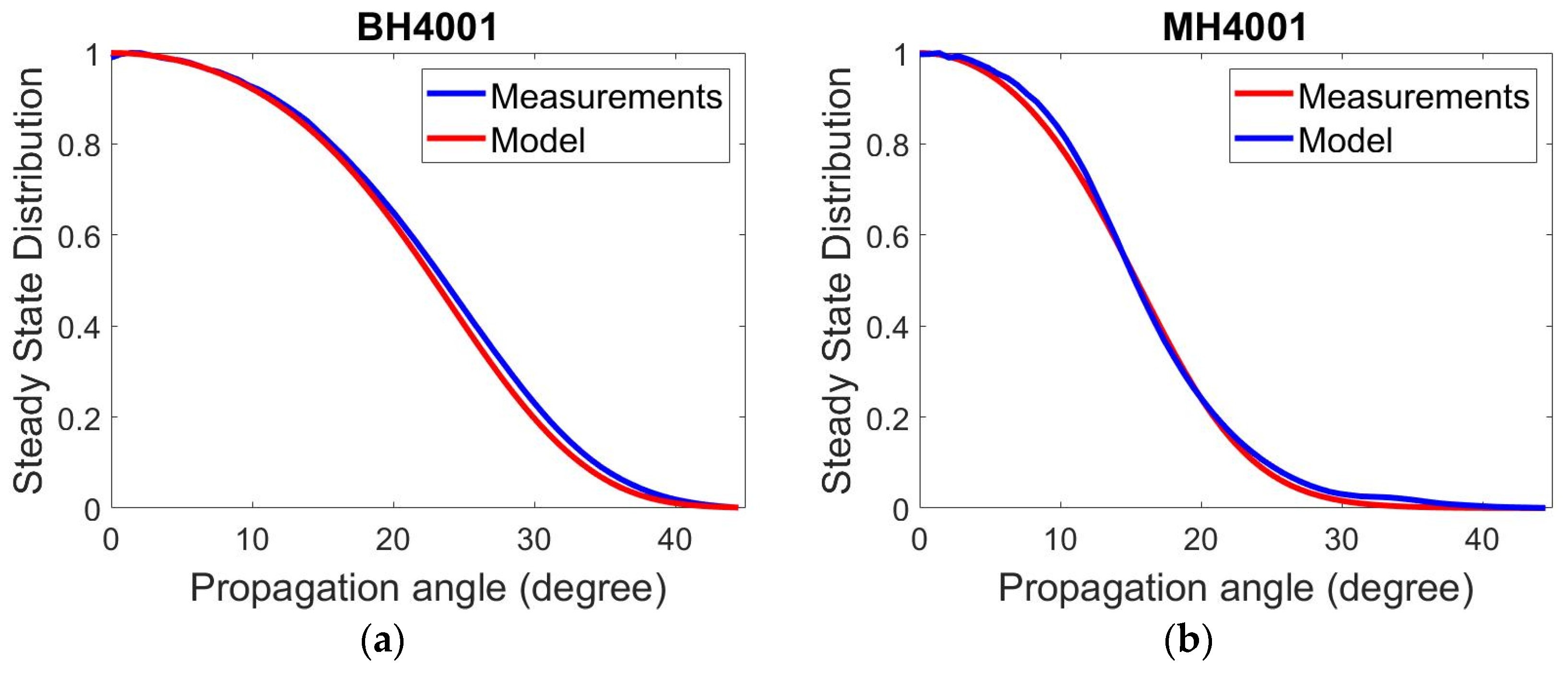
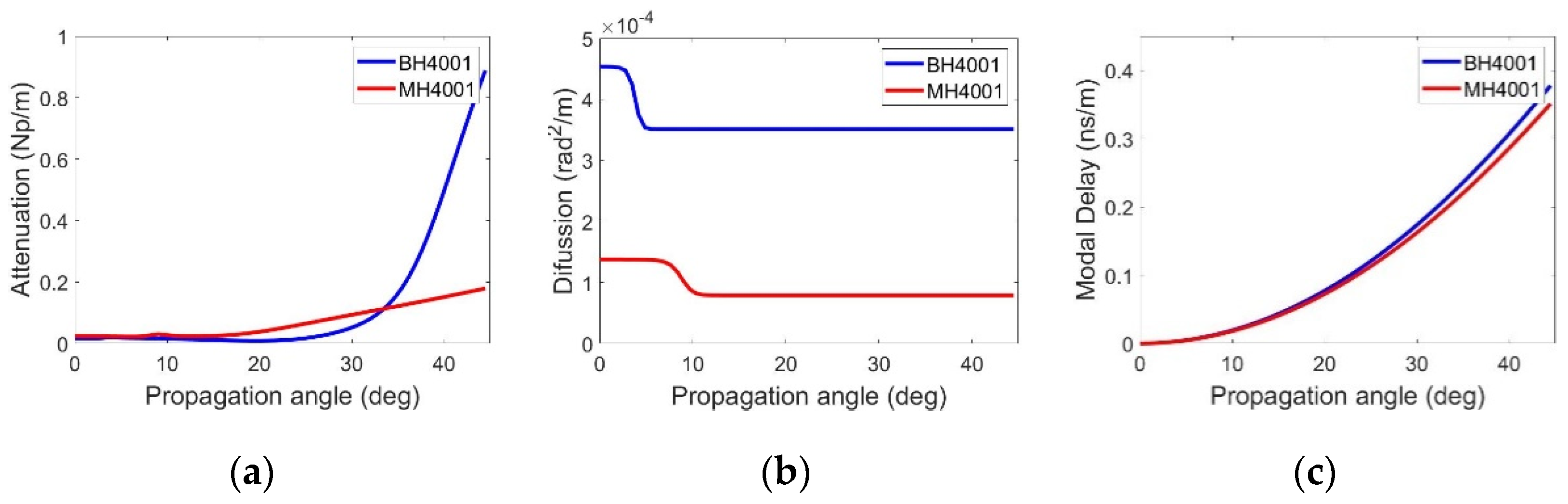
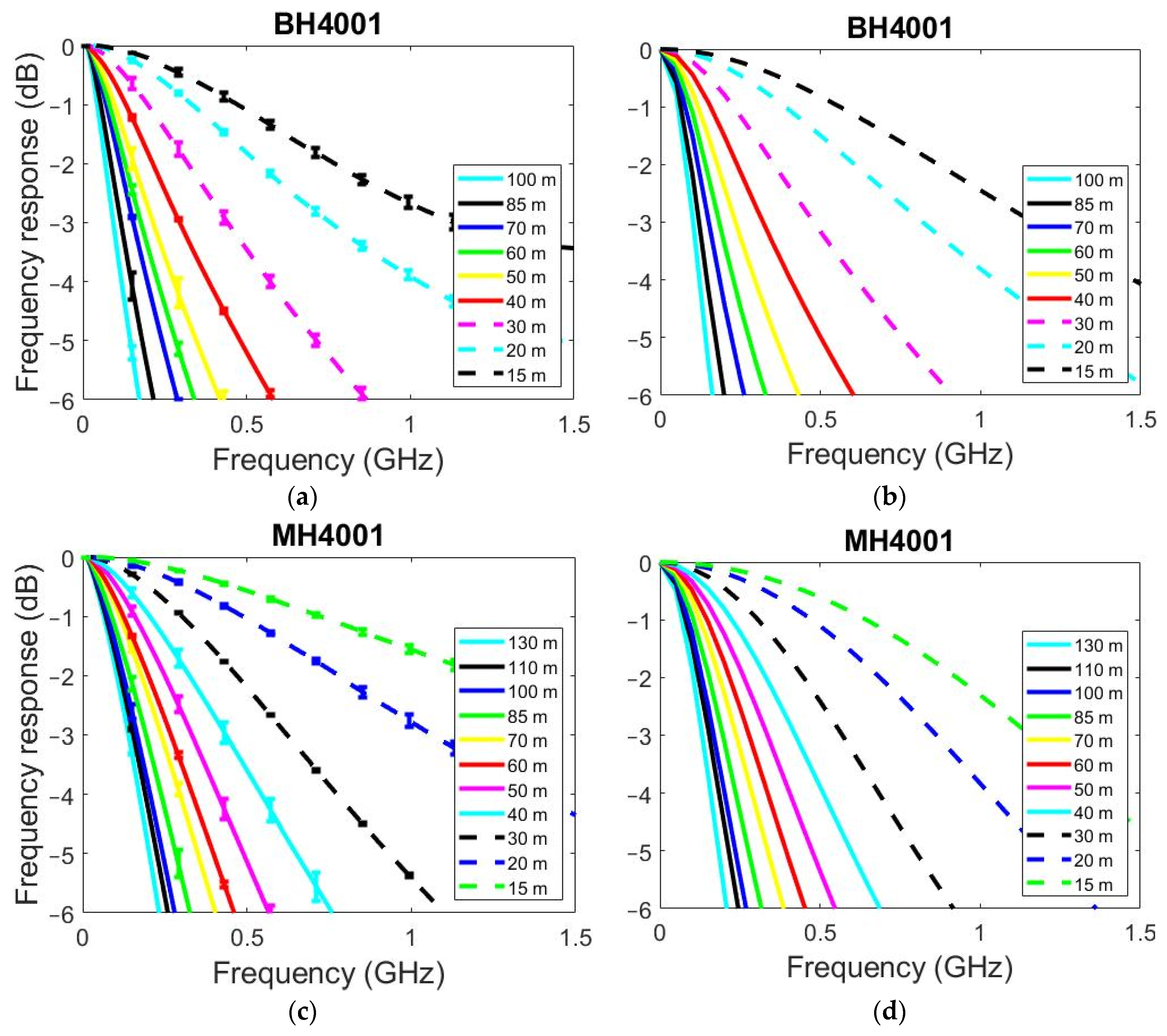
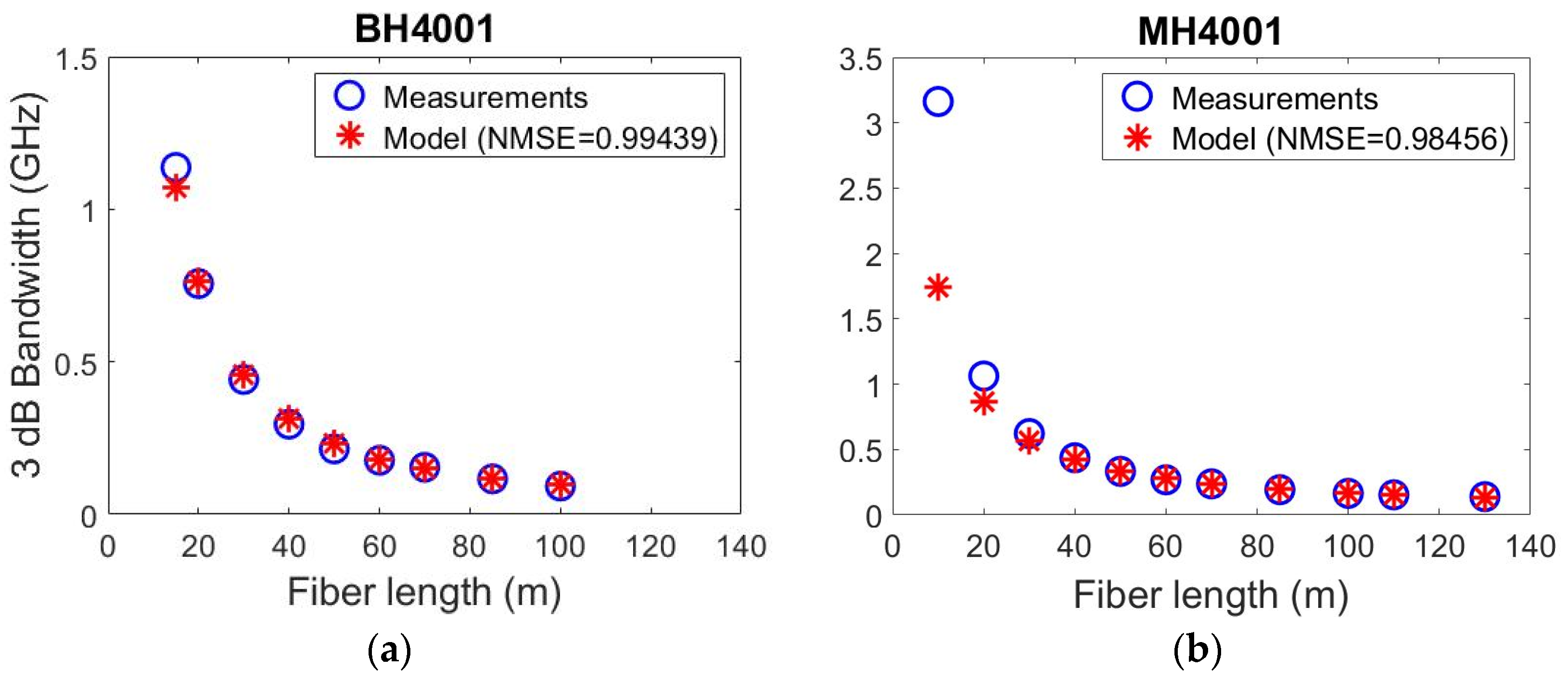
4. Results and Discussion

In this section, we show the characteristic functions for the two fibers that are calculated using the parameters obtained for the best fits. Additionally, a comparison of the experimental and model results is shown including measurements not used in the fitting algorithm.

In the proposed algorithm, the termination tolerance was set to 10⁻⁸ in order to satisfy the convergence criteria of the cost function. This tolerance is a threshold selected to guarantee that the iterative cycle breaks and the cost function can converge to an optimum value. This value is directly related to the set of parameters that best fit the characteristic functions.

Figure 3a depicts the attenuation function considering the SSD at 100 m for the BH4001 fiber (NA = 0.58 and $n_{core}$ = 1.49), and at 150 m for the MH4001 fiber (NA = 0.3 and $n_{core}$= 1.49), respectively. The attenuation function for the BH4001 and MH4001 fibers shows a relatively steady behavior for angles less than their critical angles (${\theta }_c$= 22.91° and ${\theta }_c$= 11.61° for BH4001 and MH4001 fibers, respectively). Both attenuation functions start to increase consistently around their critical angles.

Figure 3b depicts the diffusion functions for the BH4001 and MH4001 fibers, respectively, considering the same characteristics as in the attenuation functions. Firstly, the diffusion function for the BH4001 fiber is flat (constant diffusion) for angles less than 2.5°, and above 5°. Secondly, in the case of MH4001 fiber, the diffusion function is flat (constant diffusion) for angles less than 7° and above 10.5°. The most noticeable aspect is the difference in the maximum diffusion level between the two fibers. It is nearly triple for the BH4001 fiber. We argue that this behavior can be explained in view of the fact that the BH4001 is a temperature-resistant fiber with a thermoset jacket, while the MH4001 has a polyethylene jacket and a double cladding structure to reduce its aperture. These differences are also revealed by the parameters obtained for the diffusion functions described in Equation (9) and given in

Table 2. Parameters for the fit of the sigmoid diffusion function for the BH4001 and MH4001 fibers.

Fiber	${\mathit{D}}_0({\mathbf{rad}}^2/\mathbf{m})$	${\mathit{D}}_1({\mathbf{rad}}^2/\mathbf{m})$	${{\mathit{D}}_2}_{ }$	${\mathit{\sigma }}_{\mathit{d}}\left({\mathbf{rad}}^{-1}\right)$
BH4001	3.5114 × 10−4	1.0250 × 10−4	3 × 10−3	52.8281
MH4001	7.8954 × 10−5	5.8804 × 10−5	8.2867 × 10−4	26.0533

.

Finally, Figure 3c depicts the group delay as a function of the propagation angle for the BH4001 and MH4001 fibers, respectively revealing only slight differences.

The parameters that best fit the overall attenuation $\gamma$ and the $m_d$ factor are given in

Table 3. Parameters of the overall attenuation and mode delay characteristic functions for the BH4001 and MH4001 fibers.

Fiber	$\mathit{\gamma }$ (Np/m)	$\mathit{\gamma }$ (dB/m)	${\mathit{m}}_{\mathit{d}}$
BH4001	0.0258	0.0961	0.5496
MH4001	0.0307	0.1513	0.5310

. These parameters are described in Equations (11) and (13). Table 3 reveals a difference in the overall attenuation between the two fibers for a 520 nm wavelength. These results are consistent with previous estimates [1,27] and lower than the attenuation in the red region of the spectrum for both fibers (see characteristic sheets). In the case of the $m_d$ parameter that weights the mode delay, the results for the two fibers are quite similar.

In order to show the goodness of the fit, we compared measured and modeled frequency responses for the two fibers. Figure 4a,b depict the frequency response measurements and modeled frequency responses for the BH4001 fiber, respectively. Figure 4c,d depict the frequency response measurements and modeled frequency responses for the MH4001 fiber, respectively. The parameters shown in the previous tables were used to estimate the modeled results shown in Figure 4b,d.

Notice that only fiber lengths from 40 m to 100 m for the BH4001 and 40 m to 130 m for the MH4001 were used in the fits. These curves are shown with solid lines. The frequency responses for fiber lengths of 30, 20, and 15 m that were not introduced in the fitting algorithm are shown with dashed lines in all figures. The results show the expected behavior of the frequency response for the two types of fibers. Due to the effect of modal dispersion, the results tend to narrow with the increase of the fiber lengths. A comparison among the frequency responses reveals that the MH4001 fiber has a flatter tendency at all lengths. This is due to its lower numerical aperture (NA = 0.3) that reduces its modal dispersion.

Figure 4 shows that the model closely follows the trend of the measurements for the fiber lengths included in the fitting algorithm. However, there is a deviation for the shorter fiber lengths that is more noticeable in the MH4001 fiber, particularly for the 15 m fiber length. The fact that the model does not precisely follow experimental frequency responses for short fibers is not a crucial factor. In fact, it has been shown that experimental measurements of short fibers display large variability. They can be modeled using a statistical approach [37]. This behavior can be expected due to the fact that the impact of curvatures, fiber end termination, detector position, etc., over transmission properties is more significant for short fibers.

Figure 5 depicts the 3 dB bandwidth as a function of fiber length for (a) the BH4001, and (b) the MH4001 fibers, respectively. The bandwidths obtained from the experimental measurements are represented by the blue circles, and those obtained from the frequency responses generated using the model are represented by the red stars.

Figure 5 shows a good agreement between experimental and modeled results except in the case of the bandwidth for the 15 m length in the MH4001 fiber. This behavior is consistent with the frequency responses above. In order to validate the modeling approach, a goodness of fit test was computed between the measurements and modeled results. In this validation, we used the normalized root mean square error ($NMSE$) as a cost function, i.e., we computed the following value:

$$NMSE=1-\frac{||xref-{x||}^2}{||xref-mean{\left(xref\right)||}^2},$$

(18)

where $x$ accounts for the results to be tested and $xref$ is the reference data. The value of $NMSE$ varies between -Inf (bad fit) to 1 (perfect fit).

In the case of the BH4001 fiber, a comparison between the experimental measurements and the results generated by the model reveals that the 3 dB frequency response fit cost is 0.9944. The fit cost takes into consideration the fiber lengths from 15 m to 100 m. In the case of the MH4001 fiber, the fit cost is 0.9806, and it takes into consideration fiber lengths from 15 m to 130 m. In both cases, the data for the three fiber lengths that were not used in the fit (15, 20, and 30 m) are included in the fit cost calculation. The results for both fibers show a reasonable accuracy of the computational modeling algorithm used to generate the transmission characteristics.

Figure 6 depicts the received optical power as a function of fiber length for the two fibers. The blue circles represent the direct measurements obtained in the cut-back experiment for each fiber length using the power-meter. In the cut-back experiment, we performed at least five direct measurements of the output power at each fiber length. The bars represent the standard deviation of these data. The red stars represent the received power calculated in Equation (15) using the intensity distributions generated by the model. Additionally, the overall attenuation, $\gamma$, is given by the slope of the optical power versus length. The slope of the blue and red lines represents the overall attenuation of the measured and modeled optical power vs. length, respectively.

It is relevant to highlight that the measurements of received power were not used in the fitting algorithm. The received power was calculated from the intensity distributions obtained from the measured FFPs using Equation (15). Figure 6 shows good agreement between the model and the measurements. However, the received power measurements show some deviations from the linear trend in the case of the MH4001 fiber. Additionally, the error bars are larger in the MH4001 fiber. This reveals a higher variability. We observed that for this type of fiber, the fiber termination procedure of cutting, stripping, and particularly polishing can produce large changes. This is probably because of its double cladding structure.

In the case of the BH4001 fiber, a comparison between the experimental measurements and the model generated by the proposed algorithm reveals that the fit cost is 0.9925. The overall attenuation of the measured optical power obtained as the slope of the linear fit is 0.0909 dB/m. This value in comparison with the value shown in Table 3 gives us an error of 5.41%. In the case of the MH4001 fiber, the fit cost is 0.9720. The overall attenuation of the measured optical power is 0.1522 dB/m, and a comparison with the value of Table 3 shows an error of ~0.59%. The average error of the overall attenuation for the two fibers is ~3%. Although the cost function shown in Equation (17) does not include the direct optical power measurement for its calculation, the results exhibit the robustness of the proposed algorithm to model with reasonable accuracy the received optical power.

5. Conclusions

This article proposed a novel computation algorithm to estimate the fiber characteristic functions (diffusion, attenuation, and mode group delay) of standard PMMA large-core SI-POFs. The key factor that we would like to highlight is the auspicious accuracy achieved (above 97%) in the estimation process. This was revealed by the goodness of fit test that used the NMSE as a cost function. Particularly, the algorithm produced an average fit cost of 0.9895 for the modeled 3 dB bandwidth results and 0.9823 for the modeled optical power results. The use of the MEM approach showed a computationally efficient behavior to satisfactorily calculate the modeled results in both fibers. These results showed the expected behavior along the propagation angle. Moreover, the selection of the proper cost function played a relevant role in the computational efficiency and the accuracy of the results. Our findings prove the robustness of the proposed computational algorithm, and it gives us the confidence to state that it can be reliably used to model various types of SI-POFs. Finally, our next goals are to test the robustness of the computational algorithm using both GI-POFs and multicore POFs and to analyze the impact of the modal delay function on the frequency response results.

References

1. Ziemann, O.; Krauser, J.; Zamzowr, P.E.; Daum, W. Application of Polymer Optical and Glass Fibers. In POF Handbook: Optical Short Range Transmission Systems, 2nd ed.; Springer: Berlin/Heidelberg, Germany, 2008. [Google Scholar]
2. Mateo, J.; Losada, M.A.; López, A. POF misalignment model based on the calculation of the radiation pattern using the Hankel transform. Opt. Express 2015, 23, 8061. [Google Scholar] [CrossRef] [PubMed] [Green Version]
3. Losada, M.A.; López, A.; Mateo, J. Attenuation and diffusion produced by small-radius curvatures in POFs. Opt. Express 2016, 24, 15710. [Google Scholar] [CrossRef] [PubMed]
4. Shi, Y.; Tangdiongga, E.; Koonen, A.M.J.; Bluschke, A.; Rietzsch, P.; Montalvo, J.; De Laat, M.M.; Hoven, G.N.V.D.; Huiszoon, B. Plastic-optical-fiber-based in-home optical networks. IEEE Commun. Mag. 2014, 52, 186–193. [Google Scholar] [CrossRef]
5. Mittal, N.; Shah, M.; John, J. A low cost short haul plastic optical fiber link for home networking applications. In Proceedings of the 2016 IEEE International Conference on Recent Trends in Electronics, Information & Communication Technology (RTEICT), Bengaluru, India, 20–21 May 2016; pp. 2112–2116. [Google Scholar] [CrossRef]
6. Nazaretian, R.; Molen, G.M. Reducing Vehicle Weight and Improving Security by Using Plastic Optical Fiber. In Proceedings of the 2015 IEEE Vehicle Power and Propulsion Conference (VPPC), Montreal, QC, Canada, 19–22 October 2015; pp. 1–6. [Google Scholar] [CrossRef]
7. López, A.; Losada, M.Á.; Mateo, J.; Jiang, X.; Richards, D.H.; Antoniades, N. Transmission Performance of Plastic Optical Fibers Designed for Avionics Platforms. J. Lightwave Technol. 2018, 36, 5082–5088. [Google Scholar] [CrossRef] [Green Version]
8. Sercos Technology. Available online: https://www.sercos.org/technology/ (accessed on 24 January 2022).
9. Theodosiou, A.; Kalli, K. Recent trends and advances of fibre Bragg grating sensors in CYTOP polymer optical fibres. Opt. Fiber Technol. 2020, 54, 102079. [Google Scholar] [CrossRef]
10. Marques, C.A.F.; Min, R.; Junior, A.L.; Antunes, P.; Fasano, A.; Woyessa, G.; Nielsen, K.; Rasmussen, H.K.; Ortega, B.; Bang, O. Fast and stable gratings inscription in POFs made of different materials with pulsed 248 nm KrF laser. Opt. Express 2018, 26, 2013–2022. [Google Scholar] [CrossRef] [Green Version]
11. Hu, X.; Chen, Y.; Gao, S.; Min, R.; Woyessa, G.; Bang, O.; Qu, H.; Wang, H.; Caucheteur, C. Direct Bragg Grating Inscription in Single Mode Step-Index TOPAS/ZEONEX Polymer Optical Fiber Using 520 nm Femtosecond Pulses. Polymers 2022, 14, 1350. [Google Scholar] [CrossRef]
12. Junior, A.L.; Frizera, A.; Marques, C.; Sanchez, M.R.A.; Dos Santos, W.M.; Siqueira, A.A.G.; Segatto, M.V.; Pontes, M. Polymer Optical Fiber for Angle and Torque Measurements of a Series Elastic Actuator’s Spring. J. Lightwave Technol. 2018, 36, 1698–1705. [Google Scholar] [CrossRef]
13. Koyama, S.; Haseda, Y.; Ishizawa, H.; Okazaki, F.; Bonefacino, J.; Tam, H.-Y. Measurement of Pulsation Strain at the Fingertip Using a Plastic FBG Sensor. IEEE Sens. J. 2021, 21, 21537–21545. [Google Scholar] [CrossRef]
14. Leal-Junior, A.G.; Díaz, C.R.; Marques, C.; Pontes, M.J.; Frizera, A. Multiplexing technique for quasi-distributed sensors arrays in polymer optical fiber intensity variation-based sensors. Opt. Laser Technol. 2018, 111, 81–88. [Google Scholar] [CrossRef]
15. Graded-Index Polymer Optical Fiber (GI-POF). Available online: https://www.thorlabs.com/catalogpages/v20/892.pdf (accessed on 1 December 2021).
16. Loquai, S.; Kruglov, R.; Schmauss, B.; Bunge, C.-A.; Winkler, F.; Ziemann, O.; Hartl, E.; Kupfer, T. Comparison of Modulation Schemes for 10.7 Gb/s Transmission Over Large-Core 1 mm PMMA Polymer Optical Fiber. J. Light. Technol. 2013, 31, 2170–2176. [Google Scholar] [CrossRef]
17. Gimeno, C.; Guerrero, E.; Sánchez-Azqueta, C.; Royo, G.; Aldea, C.; Celma, S. Continuous-Time Linear Equalizer for Multigigabit Transmission Through SI-POF in Factory Area Networks. IEEE Trans. Ind. Electron. 2015, 62, 6530–6532. [Google Scholar] [CrossRef]
18. Koike, K.; Koike, Y. Design of Low-Loss Graded-Index Plastic Optical Fiber Based on Partially Fluorinated Methacrylate Polymer. J. Light. Technol. 2009, 27, 41–46. [Google Scholar] [CrossRef]
19. Gloge, D. Optical Power Flow in Multimode Fibers. Bell Syst. Tech. J. 1972, 51, 1767–1783. [Google Scholar] [CrossRef]
20. Drljača, B.; Djordjevich, A.; Savović, S. Frequency response in step-index plastic optical fibers obtained by numerical solution of the time-dependent power flow equation. Opt. Laser Technol. 2012, 44, 1808–1812. [Google Scholar] [CrossRef]
21. Djordjevich, A.; Savovic, S. Investigation of mode coupling in step index plastic optical fibers using the power flow equation. IEEE Photonics Technol. Lett. 2000, 12, 1489–1491. [Google Scholar] [CrossRef]
22. Mateo, J.; Losada, M.A.; Garcés, I.; Zubia, J. Global characterization of optical power propagation in step-index plastic optical 484 fibers. Opt. Express 2006, 14, 9028–9035. [Google Scholar] [CrossRef]
23. Richards, D.H.; Losada, M.A.; Antoniades, N.; Lopez, A.; Mateo, J.; Jiang, X.; Madamopoulos, N. Modeling Methodology for Engineering SI-POF and Connectors in an Avionics System. J. Light. Technol. 2013, 31, 468–475. [Google Scholar] [CrossRef]
24. Stepniak, G.; Siuzdak, J. Modeling of transmission characteristics in step-index polymer optical fiber using the matrix exponential method. Appl. Opt. 2018, 57, 9203–9207. [Google Scholar] [CrossRef]
25. Mundus, M.; Hohl-Ebinger, J.; Warta, W. Estimation of angle-dependent mode coupling and attenuation in step-index plastic optical fibers from impulse responses. Opt. Express 2013, 21, 17077–17088. [Google Scholar] [CrossRef]
26. International Electrotechnical Commission. Optical Fibres: Part 1–40: Measurement Methods and Test Procedures: Attenuation; IEC 60793-1-40; ICE: Geneva, Switzerland, 2001. [Google Scholar]
27. Losada, M.A.; Mazo, M.; Lopez, A.; Muzas, C.; Mateo, J. Experimental assessment of the transmission performance of step index polymer optical fibers using a green laser diode. Polymers 2021, 13, 3397. [Google Scholar] [CrossRef]
28. Mitsubishi Chemical Corporation. Basic Requirements for the Structure and Optical Performances of BH-4001; BH-4001 Datasheet: Tokyo, Japan, April 2019. [Google Scholar]
29. Mitsubishi Chemical Corporation. Basic Requirements for the Structure and Optical Performances of MH-4001; MH-4001 Datasheet: Tokyo, Japan, April 2019. [Google Scholar]
30. Mateo, J.; Losada, M.A.; Zubia, J. Frequency response in step index plastic optical fibers obtained from the generalized power flow equation. Opt. Express 2009, 17, 2850–2860. [Google Scholar] [CrossRef] [PubMed]
31. Gloge, D. Impulse Response of Clad Optical Multimode Fibers. Bell Syst. Tech. J. 1973, 52, 801–816. [Google Scholar] [CrossRef]
32. Gambling, W.; Payne, D.; Matsumura, H. Mode conversion coefficients in optical fibers. Appl. Opt. 1975, 14, 1538–1542. [Google Scholar] [CrossRef] [PubMed]
33. Djordjevich, A.; Savovic, S. Numerical Solution of the Power Flow Equation in Step-Index Plastic Optical Fibers. J. Opt. Soc. Am. B USA 2004, 21, 1437–1442. [Google Scholar] [CrossRef]
34. Breyer, F.; Hanik, N.; Lee, S.; Randel, S. POF Modelling: Theory, Measurement and Application. In Getting the Impulse Response of SI-POF by Solving the Time-Dependent Power-Flow Equation Using the Crank-Nicholson Scheme; Bunge, C.A., Poisel, H., Eds.; Verlag Books on Demand GmbH: Norderstedt, Germany, 2007. [Google Scholar]
35. Djordjevich, A.; Savovic, S. Coupling length as an algebraic function of the coupling coefficient in step-index plastic optical fibers. Opt. Eng. 2008, 47, 125001. [Google Scholar] [CrossRef]
36. López, A.; Losada, A.; Mateo, J.; Zubia, J. On the Variability of Launching and Detection in POF Transmission Systems. In Proceedings of the 20th International Conference on Transparent Optical Networks (ICTON), Bucharest, Romania, 1–5 July 2018. [Google Scholar] [CrossRef]
37. Lagarias, J.C.; Reeds, J.A.; Wright, M.H.; Wright, P.E. Convergence Properties of the Nelder-Mead Simplex Method in Low Dimensions. SIAM J. Optim. 1998, 9, 112–147. [Google Scholar] [CrossRef] [Green Version]
Figure 1. Experimental setup system for measurement acquisition. (a) Optical power subsystem; (b) far field pattern images subsystem; (c) S21 transmission parameter subsystem.
Photonics 09 00260 g001
Figure 2. Normalized steady-state distribution function. (a) BH4001 fiber and (b) MH4001 fiber.
Photonics 09 00260 g002
Figure 3. Plastic optical fiber characteristic functions as a function of the propagation angle. (a) Attenuation, (b) diffusion, and (c) group delay.
Photonics 09 00260 g003
Figure 4. Normalized frequency response at selected fiber lengths. (a,c) Normalized frequency response measurements for BH4001 and MH4001 fibers respectively, (b,d) Normalized frequency response modeled results for BH4001 and MH4001 fibers respectively.
Photonics 09 00260 g004
Figure 5. 3 dB bandwidth as a function of the fiber length for (a) BH4001 fiber and (b) MH4001 fiber.
Photonics 09 00260 g005
Figure 6. Optical power as a function of the fiber length. (a) BH4001 fiber and (b) MH4001 fiber.
Photonics 09 00260 g006