On-Demand Phase Control of a 7-Fiber Amplifiers Array with Neural Network and Quasi-Reinforcement Learning

Abstract
:1. Introduction
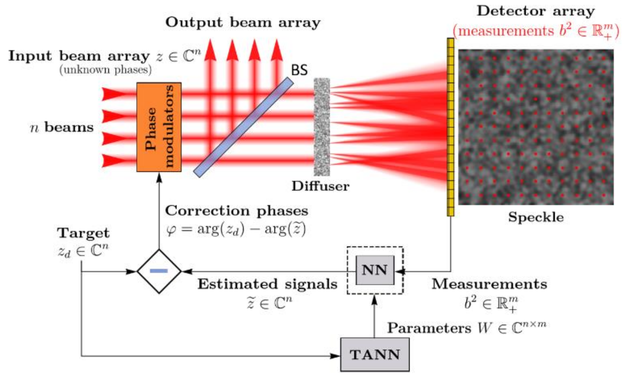
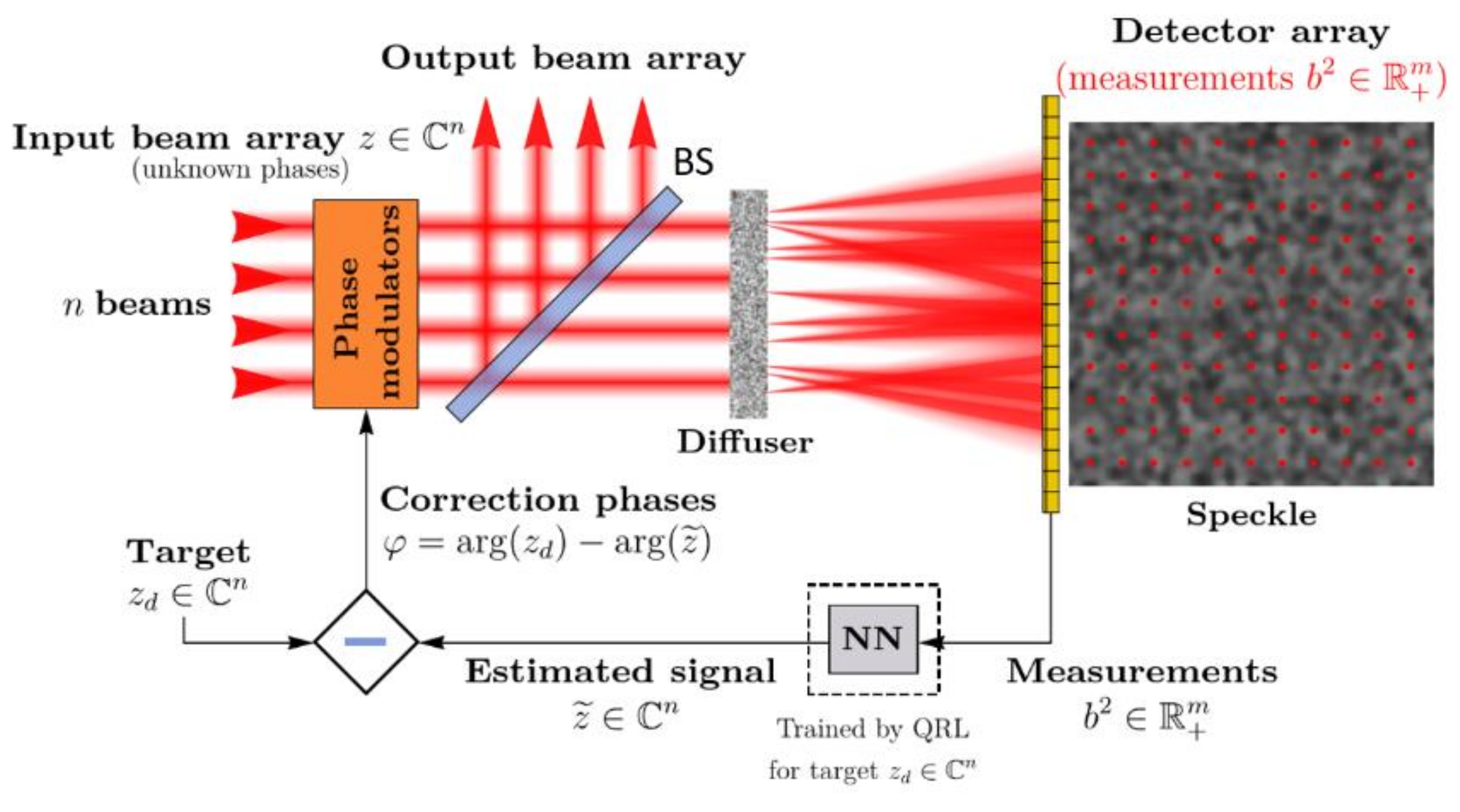
2. Neural Network in a Phase Reduction Loop with Quasi-Reinforcement Learning
3. Target Adaptive NN with QRL Process
| Algorithm 1: Quasi-reinforcement learning algorithm for TANN |
| Input: Measurement model: , reward function Output:Trained target adaptive neural network TANN:
|
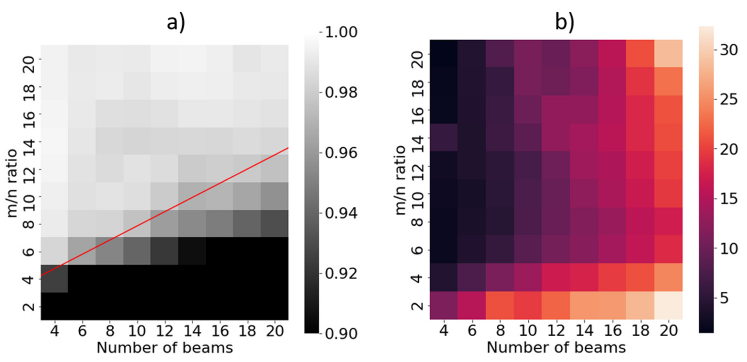
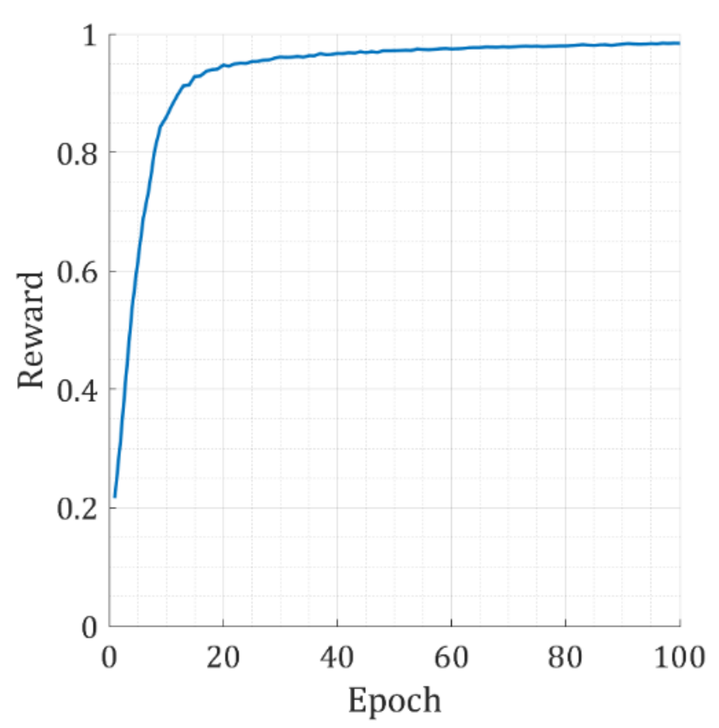
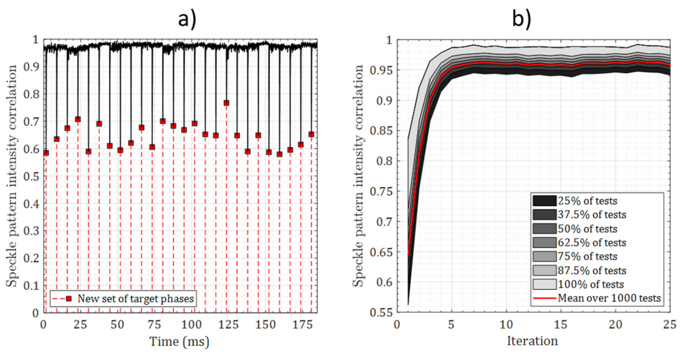
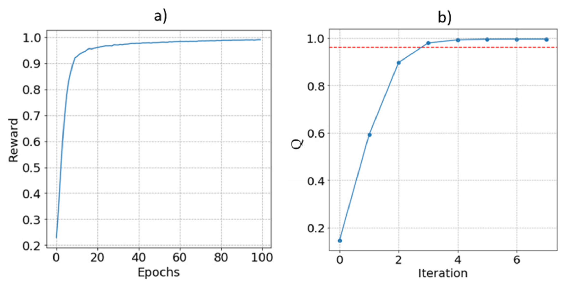
4. Simulations
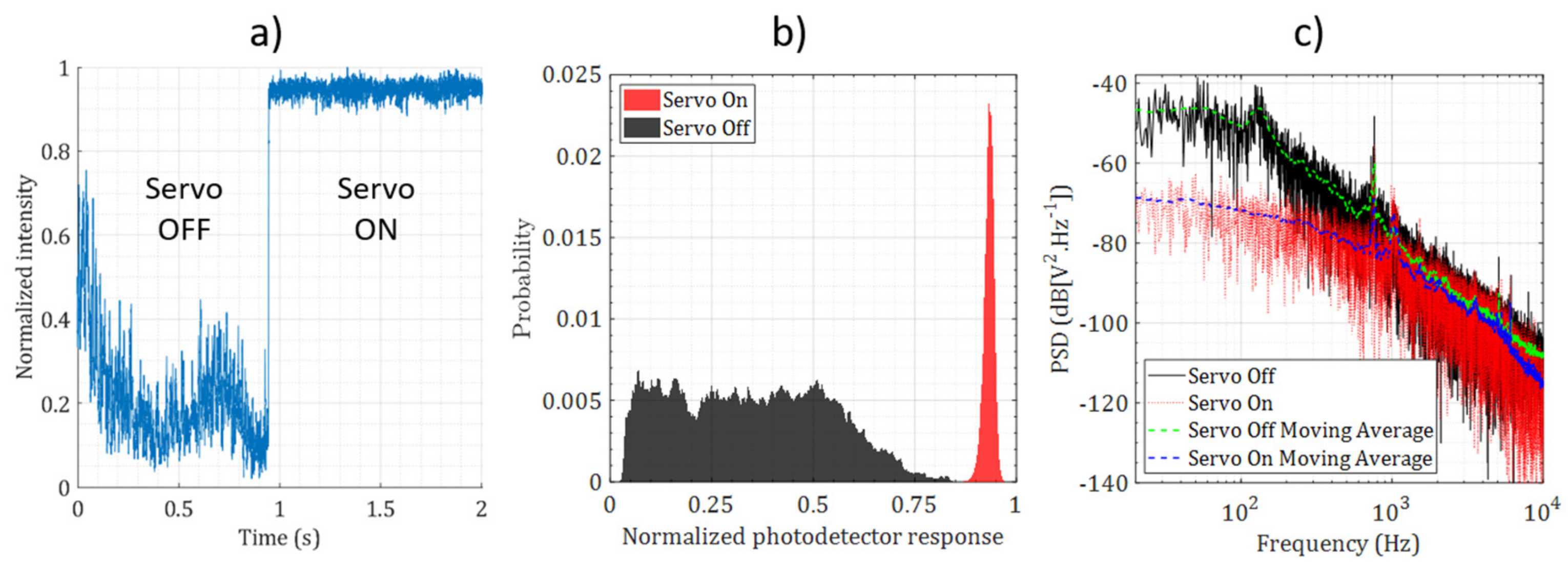
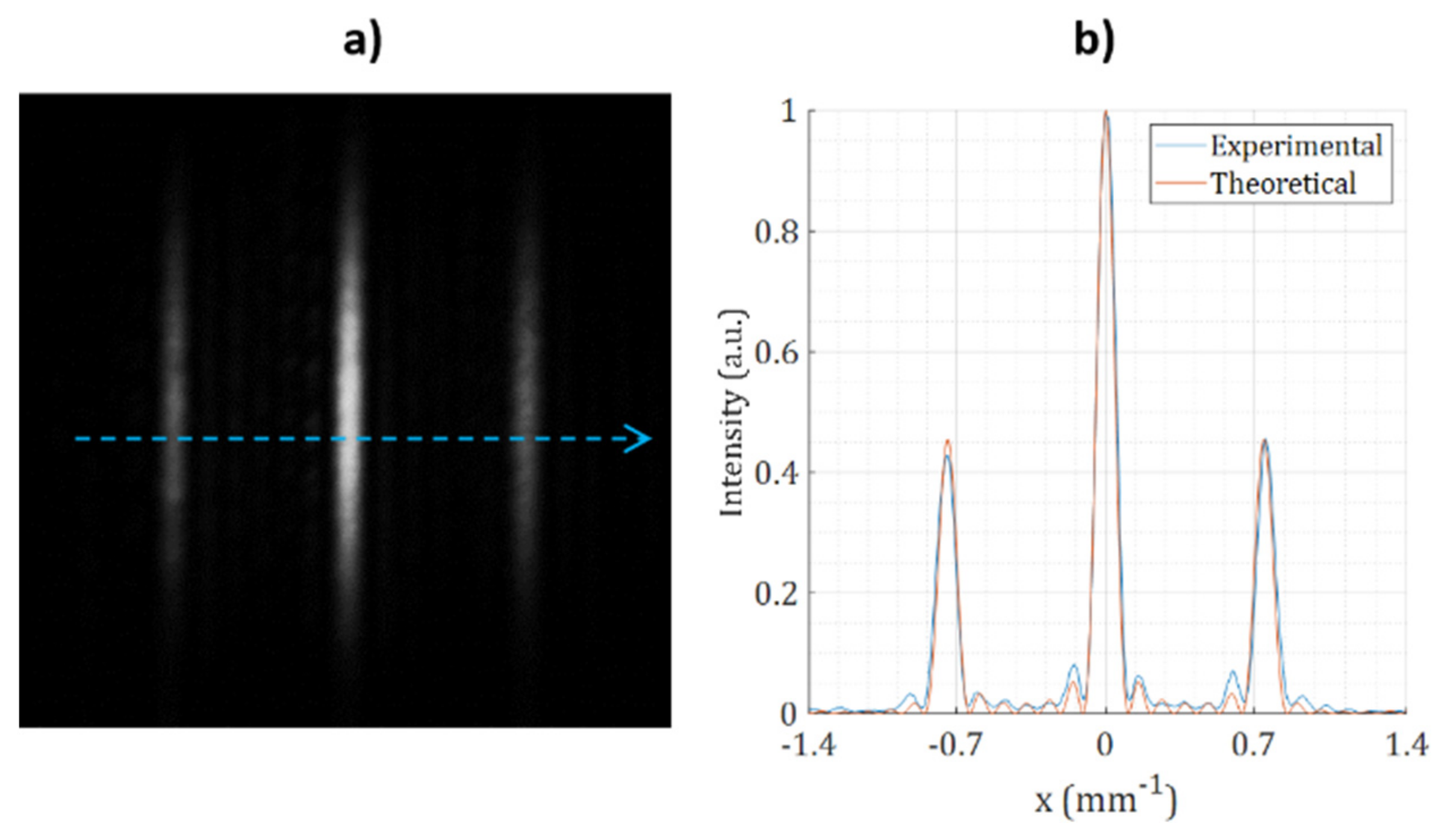
5. Experiments
6. Conclusions
Author Contributions
Funding
Data Availability Statement
Conflicts of Interest
References
- Ma, P.; Chang, H.; Ma, Y.; Su, R.; Qi, Y.; Wu, J.; Li, C.; Long, J.; Lai, W.; Chang, Q.; et al. 27.1 kW coherent beam combining system based on a seven-channel fiber amplifier array. Opt. Laser Tech. 2021, 140, 107016. [Google Scholar] [CrossRef]
- Weyrauch, T.; Vorontsov, M.; Mangano, J.; Ovchinnikov, V.; Bricker, D.; Polnau, E.; Rostov, A. Deep turbulence effects mitigation with coherent combining of 21 laser beams over 7 km. Opt. Lett. 2016, 41, 840–842. [Google Scholar] [CrossRef]
- Yang, X.; Huang, G.; Li, F.; Li, X.; Li, B.; Geng, C.; Li, X. Continuous Tracking and Pointing of Coherent Beam Combining System via Target-in-the-Loop Concept. IEEE Phot. Tech. Lett. 2021, 33, 1119–1122. [Google Scholar] [CrossRef]
- Hou, T.; Dong, Z.; Tao, R.; Ma, Y.; Zhou, P.; Liu, Z. Spatially-distributed orbital angular momentum beam array generation based on greedy algorithms and coherent combining technology. Opt. Express 2018, 26, 14945–14958. [Google Scholar] [CrossRef] [PubMed]
- Veinhard, M.; Bellanger, S.; Daniault, L.; Fsaifes, I.; Bourderionnet, J.; Larat, C.; Lallier, E.; Brignon, A.; Chanteloup, J.C. Orbital angular momentum beams generation from 61 channels coherent beam combining femtosecond digital laser. Opt. Lett. 2021, 46, 25–28. [Google Scholar] [CrossRef] [PubMed]
- Bourderionnet, J.; Bellanger, C.; Primot, J.; Brignon, A. Collective coherent phase combining of 64 fibers. Opt. Express 2011, 19, 17053–17058. [Google Scholar] [CrossRef]
- Shay, T.M.; Benham, V.; Baker, J.T.; Ward, B.; Sanchez, A.D.; Culpepper, M.A.; Pilkington, D.; Spring, J.; Nelson, D.J.; Lu, C.A. First experimental demonstration of self-synchronous phase locking of an optical array. Opt. Express 2006, 14, 12015–12021. [Google Scholar] [CrossRef] [PubMed]
- Vorontsov, M.A.; Carhart, G.W.; Ricklin, J.C. Adaptive phase-distortion correction based on parallel gradient-descent optimization. Opt. Lett. 1997, 22, 907–909. [Google Scholar]
- Vorontsov, M.A.; Sivokon, V. Stochastic parallel-gradient-descent technique for high-resolution wave-front phase-distortion correction. J. Opt. Soc. Am. A. 1998, 15, 2745–2758. [Google Scholar] [CrossRef]
- Yu, C.; Augst, S.; Redmond, S.; Goldizen, K.C.; Murphy, D.; Sanchez, A.; Fan, T. Coherent combining of a 4 kw, eight-element fiber amplifier array. Opt. Lett. 2011, 36, 2686–2688. [Google Scholar] [CrossRef] [PubMed]
- Zhou, P.; Liu, Z.; Wang, X.; Ma, Y.; Ma, H.; Xu, X.; Guo, S. Coherent beam combining of fiber amplifiers using stochastic parallel gradient descent algorithm and its application. IEEE J. Sel. Top. Quantum Electron 2009, 15, 248–256. [Google Scholar] [CrossRef]
- Kabeya, D.; Kermene, V.; Fabert, M.; Benoist, J.; Saucourt, J.; Desfarges-Berthelemot, A.; Barthélémy, A. Efficient phase-locking of 37 fiber amplifiers by phase-intensity mapping in an optimization loop. Opt. Express 2017, 25, 13816–13821. [Google Scholar] [CrossRef]
- Boju, A.; Maulion, G.; Saucourt, J.; Leval, J.; Ledortz, J.; Koudoro, A.; Berthomier, J.-M.; Naiim-Habib, M.; Armand, P.; Kermene, V.; et al. Small footprint phase locking system for a large tiled aperture laser array. Opt. Express 2021, 29, 11445–11452. [Google Scholar] [CrossRef] [PubMed]
- Saucourt, J.; Armand, P.; Kermène, V.; Desfarges-Berthelemot, A.; Barthélémy, A. Random Scattering and Alternating Projection Optimization for Active Phase Control of a Laser Beam Array. IEEE Photonics J. 2019, 11, 1503909. [Google Scholar] [CrossRef]
- Tunnermann, H.; Shirakawa, A. Deep reinforcement learning for coherent beam combining applications. Opt. Express 2019, 27, 24223–24230. [Google Scholar] [CrossRef] [PubMed]
- Hou, T.; An, Y.; Chang, Q.; Ma, P.; Li, J.; Zhi, D.; Huang, L.; Su, R.; Wu, J.; Ma, Y.; et al. Deep Learning-based phase control method for coherent beam combining systems. High Power Laser Sci. Eng. 2019, 7, e59. [Google Scholar] [CrossRef] [Green Version]
- Chang, Q.; An, Y.; Hou, T.; Su, R.; Ma, P.; Zhou, P. Phase-locking System in Fiber Laser Array through Deep Learning with Diffusers, Paper M4A.96. In Proceedings of the Asia Communications and Photonics Conference, Beijing, China, 24–27 October 2020. [Google Scholar]
- Hou, T.; An, Y.; Chang, Q.; Ma, P.; Li, J.; Huang, L.; Zhi, D.; Wu, J.; Su, R.; Ma, Y.; et al. Deep-learning-assisted, two-stage phase control method for high-power mode-programmable orbital angular momentum beam generation. Photonics Res. 2020, 8, 715–722. [Google Scholar] [CrossRef]
- Tünnermann, H.; Shirakawa, A. Deep reinforcement learning for tiled aperture beam combining in a simulated environment. JPhys Photonics 2021, 3, 015004. [Google Scholar] [CrossRef]
- Wang, D.; Du, Q.; Zhou, T.; Li, D.; Wilcox, R. Stabilization of the 81-channel coherent beam combination using machine learning. Opt. Express 2021, 29, 5694–5709. [Google Scholar] [CrossRef] [PubMed]
- Zhang, X.; Li, P.; Zhu, Y.; Li, C.; Yao, C.; Wang, L.; Dong, X.; Li, S. Coherent beam combination based on Q-learning algorithm. Opt. Comm. 2021, 490, 126930. [Google Scholar] [CrossRef]
- Shpakovych, M.; Maulion, G.; Kermene, V.; Boju, A.; Armand, P.; Desfarges-Berthelemot, A.; Barthélemy, A. Experimental phase control of a 100 laser beam array with quasi-reinforcement learning of a neural network in an error reduction loop. Opt. Express 2021, 29, 12307–12318. [Google Scholar] [CrossRef]
- Nabors, C. Effects of phase errors on coherent emitter arrays. Appl. Optics. 1994, 33, 2284–2289. [Google Scholar] [CrossRef]
- PPopoff, S.; Lerosey, M.G.; Carminati, R.; Fink, M.; Boccara, C.; Gigan, S. Measuring the transmission matrix in optics: An approach to the study and control of light propagation in disordered media. Phys. Rev. Lett. 2010, 104, 100601. [Google Scholar] [CrossRef]
- Drémeau, A.; Liutkus, A.; Martina, D.; Katz, O.; Schülke, C.; Krzakala, F.; Gigan, S.; Daudet, L. Reference-less measurement of the transmission matrix of a highly scattering material using a DMD and phase retrieval techniques. Opt. Express 2015, 23, 11898–11911. [Google Scholar] [CrossRef] [Green Version]


Publisher’s Note: MDPI stays neutral with regard to jurisdictional claims in published maps and institutional affiliations. |
© 2022 by the authors. Licensee MDPI, Basel, Switzerland. This article is an open access article distributed under the terms and conditions of the Creative Commons Attribution (CC BY) license (https://creativecommons.org/licenses/by/4.0/).
Share and Cite
Shpakovych, M.; Maulion, G.; Boju, A.; Armand, P.; Barthélémy, A.; Desfarges-Berthelemot, A.; Kermene, V. On-Demand Phase Control of a 7-Fiber Amplifiers Array with Neural Network and Quasi-Reinforcement Learning. Photonics 2022, 9, 243. https://doi.org/10.3390/photonics9040243
Shpakovych M, Maulion G, Boju A, Armand P, Barthélémy A, Desfarges-Berthelemot A, Kermene V. On-Demand Phase Control of a 7-Fiber Amplifiers Array with Neural Network and Quasi-Reinforcement Learning. Photonics. 2022; 9(4):243. https://doi.org/10.3390/photonics9040243
Chicago/Turabian StyleShpakovych, Maksym, Geoffrey Maulion, Alexandre Boju, Paul Armand, Alain Barthélémy, Agnès Desfarges-Berthelemot, and Vincent Kermene. 2022. "On-Demand Phase Control of a 7-Fiber Amplifiers Array with Neural Network and Quasi-Reinforcement Learning" Photonics 9, no. 4: 243. https://doi.org/10.3390/photonics9040243
APA StyleShpakovych, M., Maulion, G., Boju, A., Armand, P., Barthélémy, A., Desfarges-Berthelemot, A., & Kermene, V. (2022). On-Demand Phase Control of a 7-Fiber Amplifiers Array with Neural Network and Quasi-Reinforcement Learning. Photonics, 9(4), 243. https://doi.org/10.3390/photonics9040243