Modeling for Generating Femtosecond Pulses in an Er-Doped Fiber Using Externally Controlled Spectral Broadening and Compression Mechanisms

Abstract

A model for generating femtosecond laser pulses from a low-power mode-locked laser of moderate temporal half-width was proposed. This was achieved by injecting the pulse into a single-mode inverted-populated Er-doped fiber where self-focusing and absorption were avoided. To initiate spectral broadening, the pulse was phase-modulated by subjecting a part of the fiber to an electric field of suitable intensity and frequency generated into a circular capacitor. To stimulate temporal compression, the phase-modulated pulse was introduced into a combination of two prism sets located symmetrically with respect to the x-axis. After passing the pulse through the first prism set, its spectral components were spatially separated in the y-axis. The spectral phases were manipulated by redirecting the spectral components through a slab cross-section that was subjected to a spatially modulated DC electric field. After passing the slab, the pulse is directed into the second prism set, where the spectral components were spatially overlapped and propagated outside the compressor with the same slope and dimension as before entering the compressor. Constructive super positioning of the phase-manipulated spectral components gave maximum intensity only at a specified location.

1. Introduction

Since the development of mode-locked lasers, shorter pulse durations have been required for many applications in science, medicine, and engineering. Such applications are given in [1,2,3,4,5,6,7,8,9]. To direct a conventional laser pulse into a femtosecond region, it is mathematically necessary to broaden its spectral bandwidth. Because this is achievable by applying nonlinear phenomena to the pulse, different methods for its realization were presented in [10,11,12,13,14]. According to the dispersion relations of the refractive index, the frequency components comprising the spectral bandwidth of the pulse have different velocities. Each frequency will reach an observer at different times, leading either to compressing or expanding the pulse duration. Since most of the materials have a positive-group-delay dispersion (PGDD) that expands the pulse duration, a material of negative-group-delay dispersion (NGDD) is required to reduce its duration. References [15,16,17,18,19,20,21,22] have illustrated different setups for its practical realization. From the above, it is evident that mutual combinations between broadening and compression methods will theoretically yield a temporal compressed pulse. So, for instance, the authors in [23] used nonlinear phenomena to increase the spectral range of a 90 fs laser pulse in a fiber and compressed the broadened pulse by a grating compressor to 30 fs. A pulse compression ratio of 12 (from 5.4 ps to 450 fs) was reported in [24] by using self-phase modulation in a 30 m optical fiber to broaden the spectrum and a grism compressor. The result of a theoretical analysis based on the solution of the nonlinear Schrödinger equation concerning pulse compression ratio and compression pulse quality as a function of fiber length and input pulse intensity was given in [25]. The study was carried out on an optical pulse chirped in a single-mode fiber by self-phase modulation and compressed with a grating compressor. Self-phase modulation in bulk material for spectral broadening the laser pulse and chirped mirror combined with two prisms for its compression was given in [26].

From the previous cited references, it is evident that most of the researchers used:

(1)

Powerful laser pulses for internally driving nonlinear phenomena to initiate the spectral broadening of the laser pulse;

(2)

Compressors with moveable compressor elements for creating compressed pulses at a desired location.

Aim of the Work

To generate a femtosecond laser pulse from a mode-locked laser pulse of low power and moderate halfwidth, it is necessary to externally stimulate nonlinear phenomena. The present article developed a model for their realization. Section 2.1 is devoted for finding a mathematical expression for an electric field that externally phase-modulates the laser pulse during its propagation in the fiber and a setup for its experimental realization. Section 2.2 is devoted to finding a method for external variation of the spectral optical path lengths. Therefore, the spectral phases are controlled such that the pulse compression occurs at a desired location without movement any of the compressor elements. A suggested setup for the experimental realization is also included.

2. Theory

Erbium-doped fibers (EDF) were chosen for generating femtosecond laser pulses for several reasons. They show high gain, polarization-independent amplification, low intrinsic optical noise [27], stable long-term performance, and possibility of being unidirectionally and bidirectionally pumped [28]. To avoid absorption and self-focusing of the laser pulse, the selected fiber was a single-mode and inverted populated. To achieve the cited goal, the pulses had to be externally spectrally broadened during propagation in the EDF. Two prism sets and a slab (for external manipulation of the spectral phases) were responsible for temporally compressing the spectrally broadened laser pulse.

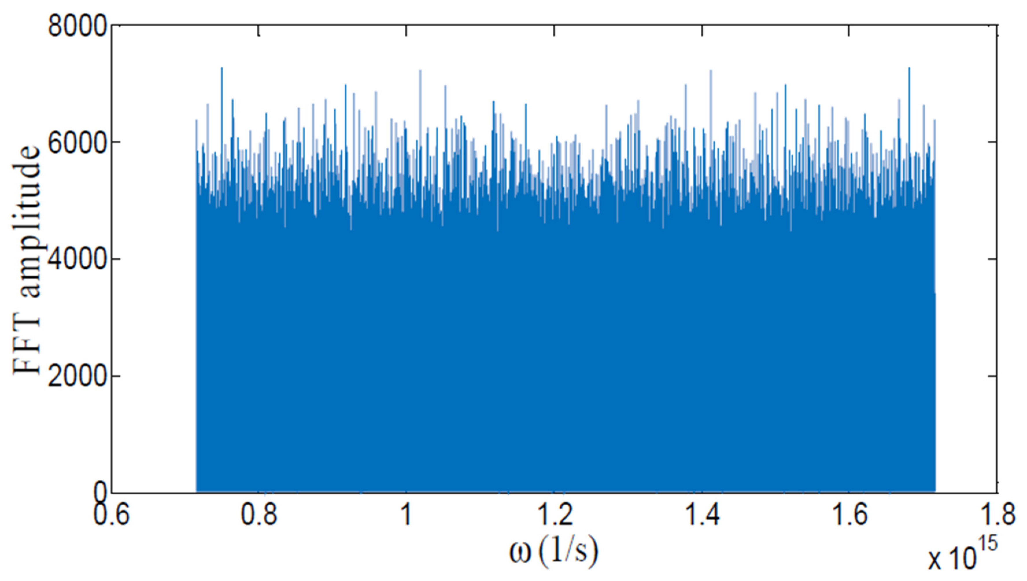
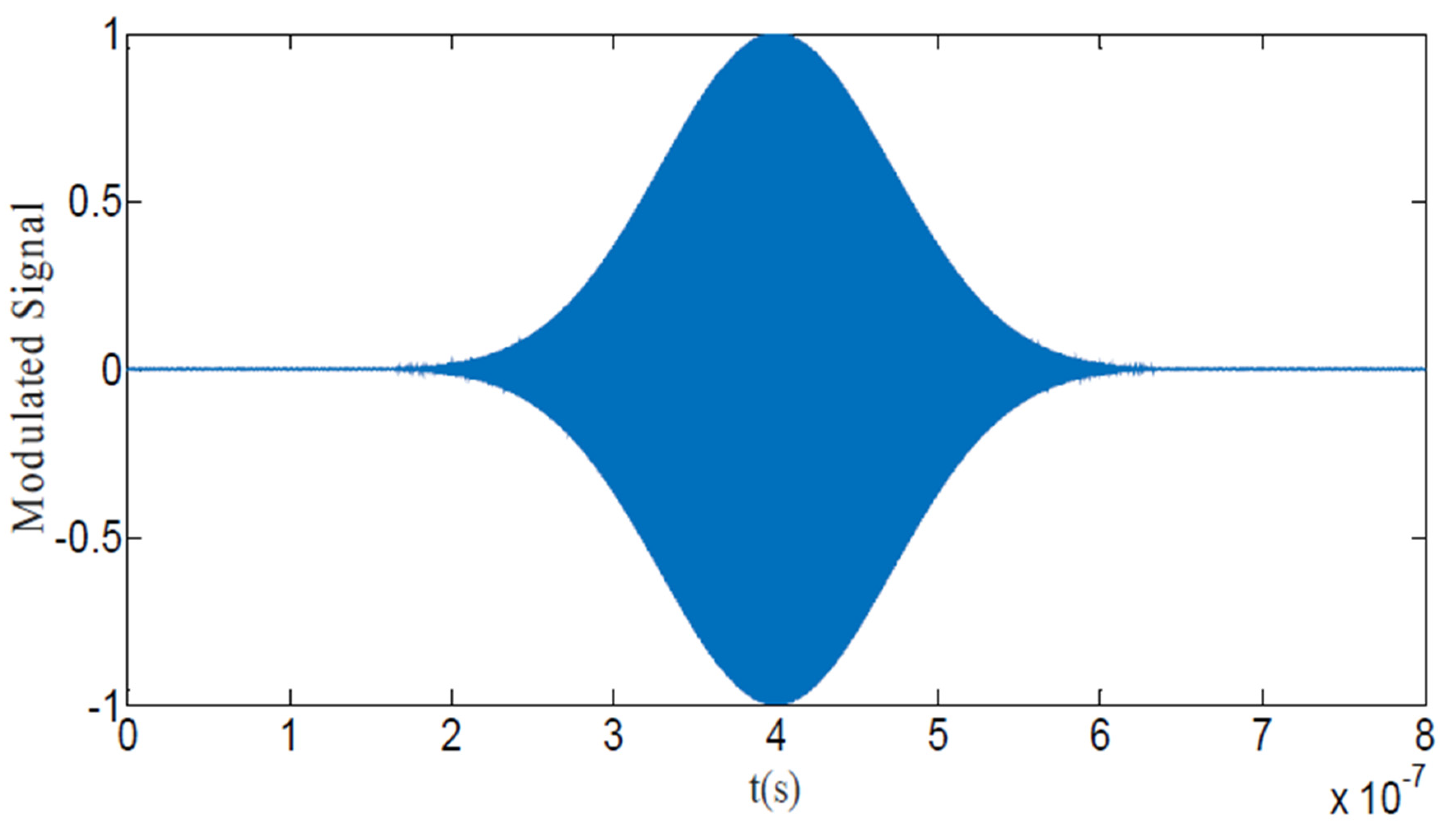
2.1. Broadening of the Spectral Bandwidth of the Laser Pulse Using an Externally Triggered Phase Modulation

A laser pulse can be coherently spectrally broadened when it is subjected to nonlinear effects either internally through self-phase modulation or externally by amplitude, frequency, or phase modulation. For a small intensity, where self-phase modulation would be ineffective, external induction of wide-range spectral broadening would be required. This was achieved by an external high-frequency electric field that modulated the refractive index of the fiber according to the following equation [29]:

$$\mathrm{n}\left(\mathsf{\Omega }\right)={ \mathrm{n}}_0\left(\mathsf{\Omega }\right)+{ \mathrm{n}}_2{\mathrm{E}}^2\left(\mathrm{t}\right),$$

(1)

where $\mathsf{\Omega }$ is the angular frequency of the electric field of the laser pulse,${ \mathrm{n}}_0\left(\mathsf{\Omega }\right)$ and ${\mathrm{n}}_2$ are the linear and nonlinear refractive indices of the fiber, respectively, and E(t) is the time-dependent external applied electric field. To create a femtosecond laser pulse, the induced spectral bandwidth (Δν), according to the Heisenberg uncertainty principle, must be in the order of 1/Δt, where Δt is the desired laser-pulse duration. To fulfill this criterion, the nonlinear part of Equation (1), ${\mathrm{n}}_2{\mathrm{E}}^2\left(\mathrm{t}\right)$, has to be in the order of the linear part ${\mathrm{n}}_0\left(\mathsf{\Omega }\right)$. This can be achieved by subjecting the fiber to a high frequency and high electric-field strength. This electric field was created by solving the Maxwell’s equations within a circular-shaped capacitor in which a part of the fiber was wrapped. The required value of the electric-field strength was obtained for certain conditions concerning the radius of the capacitor and the frequency of the generator. Due to the considered symmetry, the Maxwell’s equations have been written in cylindrical coordinates as: (detailed solution see Appendix A)

$$\frac{\partial \mathsf{{\rm E}}\left(\mathrm{r},\mathrm{t}\right)}{\partial \mathrm{r}}= \mathsf{\mu }\frac{\partial \mathrm{H}\left(\mathrm{r},\mathrm{t}\right)}{\partial \mathrm{t}},$$

(2)

$$\frac{\partial \mathrm{H}\left(\mathrm{r},\mathrm{t}\right)}{\partial \mathrm{r}}+\frac{1}{\mathrm{r}}\mathrm{H}\left(\mathrm{r},\mathrm{t}\right)= \mathsf{\epsilon }\frac{\partial \mathsf{{\rm E}}\left(\mathrm{r},\mathrm{t}\right)}{\partial \mathrm{t}}.$$

(3)

With

$$\mathrm{H}\left(\mathrm{r},\mathrm{t}\right)= \mathrm{Re}\left[\mathrm{H}\left(\mathrm{r}\right)\exp \left(\mathrm{i}\mathsf{\omega }\mathrm{t}\right)\right],$$

(4)

$$\mathsf{{\rm E}}\left(\mathrm{r},\mathrm{t}\right)= \mathrm{Re}\left[\mathrm{E}\left(\mathrm{r}\right)\exp \left(\mathrm{i}\mathsf{\omega }\mathrm{t}\right)\right],$$

(5)

it follows after setting Equations (4) and (5) into Equations (2) and (3) and applying some mathematical manipulations,

$$\frac{{\partial }^2\mathrm{H}\left(\mathrm{r}\right)}{\partial {\mathrm{r}}^2}+\frac{1}{\mathrm{r}}\frac{\partial \mathrm{H}\left(\mathrm{r}\right)}{\partial \mathrm{r}}-\frac{1}{{\mathrm{r}}^2}\mathrm{H}\left(\mathrm{r}\right)+ \mathsf{\epsilon }\mathsf{\mu }{\mathsf{\omega }}^2\mathrm{H}\left(\mathrm{r}\right)=0,$$

(6)

$$\frac{1}{\mathsf{\mu }\mathrm{i}\mathsf{\omega }}\frac{{\partial }^2\mathrm{E}\left(\mathrm{r}\right)}{\partial {\mathrm{r}}^2}+\frac{1}{\mathrm{r}}\frac{1}{\mathsf{\mu }\mathrm{i}\mathsf{\omega }}\frac{\partial \mathrm{E}\left(\mathrm{r}\right)}{\partial \mathrm{r}}- \mathsf{\epsilon }\mathrm{i}\mathsf{\omega }\mathrm{E}\left(\mathrm{r}\right)=0,$$

(7)

where $\mathsf{{\rm E}}\left(\mathrm{r},\mathrm{t}\right)$ and $\mathrm{H}\left(\mathrm{r},\mathrm{t}\right)$ are the spatial and temporal electric and magnetic field strengths, respectively, E(r) and H(r) are the spatial components of the corresponding fields, respectively, and $\mathsf{\epsilon }$ and $\mathsf{\mu }$ are the electric permittivity and magnetic permeability, respectively.

With $\mathsf{\epsilon }\mathsf{\mu }{\mathsf{\omega }}^2={ \mathrm{k}}^2$, the solution of Equations (6) and (7) are given according to [30], by

$$\mathrm{E}\left(\mathrm{r}\right)={ \mathrm{AJ}}_0\left(\mathrm{kr}\right)+{{\mathrm{A}}^{\prime }\mathrm{Y}}_0\left(\mathrm{kr}\right),$$

(8)

$$\mathrm{H}\left(\mathrm{r}\right)={ \mathrm{BJ}}_1\left(\mathrm{kr}\right)+{{\mathrm{B}}^{\prime }\mathrm{Y}}_1\left(\mathrm{kr}\right),$$

(9)

where ${\mathrm{J}}_0$ and ${\mathrm{J}}_1$ are the first kind Bessel functions of zero and first order, respectively,${\mathrm{Y}}_0{ \mathrm{and} \mathrm{Y}}_1$ are the second kind Bessel functions of zero and first order, respectively, and A and ${\mathrm{A}}^{\prime } \mathrm{as} \mathrm{well} \mathrm{as} \mathrm{B}, \mathrm{and} {\mathrm{B}}^{\prime }$ are integration constants.

To avoid the singularity of ${\mathrm{Y}}_0{ \mathrm{and} \mathrm{Y}}_1$ at $\mathrm{r} =0$, ${\mathrm{A}}^{\prime } \mathrm{and} {\mathrm{B}}^{\prime }$ were set as equal to zero. To acquire B, Ampere’s law was applied:

$$\oint \mathrm{H}\left(\mathrm{r},\mathrm{t}\right)\mathrm{rd}\mathsf{\phi } = \mathrm{Bcos}\left(\mathsf{\omega }\mathrm{t}\right){\mathrm{J}}_1\left(\mathrm{ka}\right)\left(2\mathsf{\pi }\mathrm{a}\right)=\int \frac{\partial }{\partial \mathrm{t}}\mathrm{E}\left(\mathrm{r},\mathrm{t}\right)\left(2\mathsf{\pi }\mathrm{r}\right)\mathrm{dr} = \mathrm{I}\left(\mathrm{t}\right),$$

(10)

where $\mathrm{rd}\mathsf{\phi }$ is an element of the circular path along $\mathrm{H}\left(\mathrm{r}\right)$ with radius r, a is the radius of the capacitor, and $\mathrm{I}\left(\mathrm{t}\right)$ is the feeding current of the capacitor with amplitude ${\mathrm{I}}_{\mathrm{o}}$.

Accordingly, $\mathrm{B}$ and $\mathrm{H}\left(\mathrm{r}\right)$ are determined, respectively, as:

$$\mathrm{B} ={ \mathrm{I}}_{\mathrm{o}}/\left[{\mathrm{J}}_1\left(\mathrm{ka}\right)2\mathsf{\pi }\mathrm{a}\right],$$

(11)

$$\mathrm{H}\left(\mathrm{r}\right)=\left[{\mathrm{I}}_{\mathrm{o}}/\left(2\mathsf{\pi }\mathrm{a}\right)\right]\left[{\mathrm{J}}_1\left(\mathrm{kr}\right)/{\mathrm{J}}_1\left(\mathrm{ka}\right)\right].$$

(12)

From Equation (3) and considering Equation (12), $\mathrm{E}\left(\mathrm{r}\right)$ is calculated as follows:

$$\mathrm{E}\left(\mathrm{r}\right) ={ \mathrm{I}}_{\mathrm{o}}{\mathrm{kJ}}_0\left(\mathrm{kr}\right)/\left[\left(\mathrm{i}\mathsf{\omega }\mathsf{\epsilon }\right) \left(2\mathsf{\pi }\mathrm{a}\right){\mathrm{J}}_1\left(\mathrm{ka}\right)\right],$$

(13)

With A =${ \mathrm{I}}_{\mathrm{o}}\mathrm{k}/\left[\left(\mathrm{i}\mathsf{\omega }\mathsf{\epsilon }\right)\left(2\mathsf{\pi }\mathrm{a}\right){\mathrm{J}}_1\left(\mathrm{ka}\right)\right]$, the relation between A and B is as follows:

$$\mathrm{B} = \mathrm{iA}\sqrt{\mathsf{\epsilon }/\mathsf{\mu }},$$

(14)

and the real parts of $\mathrm{E}\left(\mathrm{r},\mathrm{t}\right)$ and $\mathrm{H}\left(\mathrm{r},\mathrm{t}\right)$ can be written, respectively as

$$\mathrm{Re}\left[\mathrm{E}\left(\mathrm{r},\mathrm{t}\right)\right]= \mathrm{Re}\left[{\mathrm{AJ}}_0\left(\mathrm{kr}\right)\exp \left(\mathrm{i}\mathsf{\omega }\mathrm{t}\right)\right]={ \mathrm{I}}_{\mathrm{o}}{\mathrm{kJ}}_0\left(\mathrm{kr}\right)\sin \left(\mathsf{\omega }\mathrm{t}\right)/\left[\left(\mathsf{\omega }\mathsf{\epsilon } \left(2\mathsf{\pi }\mathrm{a}\right){\mathrm{J}}_1\left(\mathrm{ka}\right)\right)\right],$$

(15)

$$\mathrm{Re}\left[\mathrm{H}\left(\mathrm{r},\mathrm{t}\right)\right]= \mathrm{Re}[\mathrm{iA}\sqrt{\mathsf{\epsilon }/\mathsf{\mu }}{\mathrm{J}}_1\left(\mathrm{kr}\right)\exp \left(\mathrm{i}\mathsf{\omega }\mathrm{t}\right)]={ \mathrm{I}}_{\mathrm{o}}\mathrm{k}\sqrt{\mathsf{\epsilon }/\mathsf{\mu }}{\mathrm{J}}_1\left(\mathrm{kr}\right)\cos \mathsf{\omega }\mathrm{t}/\left[\mathsf{\omega }\mathsf{\epsilon } \left(2\mathsf{\pi }\mathrm{a}\right){\mathrm{J}}_1\left(\mathrm{ka}\right)\right].$$

(16)

From Equations (15) and (16), the time average of the Poynting vector within the capacitor was equal to zero. This result was in accordance with the assumption of the neglected polarization, absorption losses within the fiber, and the radiation into the surrounding. The latter can be achieved by setting the distance between the capacitor plates to be in the order of 1/100 of the wavelength of the modulating electric field. From Equation (15), it was evident that the electric field could attain large values as ${\mathrm{J}}_1\left(\mathrm{ka}\right)$ approached small values. Since this was possible for a discrete infinite number of $\left(\mathrm{ka}\right)$ values, we had to choose between those provided easily available frequencies and suitable capacitor dimensions. From the obtained results, the electric-field strength of the laser pulse was phase-modulated according to the following relation:

$${\mathrm{E}}_{\mathrm{laser}}\left(\mathrm{z},\mathrm{t}\right)={ \mathrm{c}}_1\exp \left[-{\mathrm{c}}_2{\left(\left(\mathrm{t}-{\mathrm{t}}_{\mathrm{s}}\right)/\Delta {\mathrm{t}}_{\mathrm{s}}\right)}^2\right]\times \exp ({\mathrm{i}\mathsf{\Omega }}_0\mathrm{t})\exp \left[(\frac{2\mathsf{\pi }\mathrm{i}}{{\mathsf{\lambda }}_0}) \left({\mathrm{n}}_0\left(\mathsf{\Omega }\right)\mathrm{Z}+{\mathrm{n}}_2{\mathrm{E}}^2\left(\mathrm{t}\right){\mathrm{Z}}_{\mathrm{e}}\right)\right],$$

(17)

where $\exp \left[-{\mathrm{c}}_2{\left(\left(\mathrm{t}-{\mathrm{t}}_{\mathrm{s}}\right)/\Delta {\mathrm{t}}_{\mathrm{s}}\right)}^2\right]$ is the time-dependent amplitude of the electric-field strength of the laser pulse to be phase-modulated; t_s and $\Delta {\mathrm{t}}_{\mathrm{s}}$ are the time of maximum amplitude and temporal width of the electric-field strength of the laser pulse, respectively, ${\mathsf{\Omega }}_0$ and ${\mathsf{\lambda }}_0$ are the central vacuum angular frequency and the wavelength of the laser pulse, respectively, ${\mathrm{E}}^2\left(\mathrm{t}\right)$ is the square of the phase-modulating electric field obtained in Equation (15), which is multiplied by ${\mathrm{n}}_2$ to be in the order of ${\mathrm{n}}_0\left(\mathsf{\Omega }\right)$, ${\mathrm{n}}_0$ and ${\mathrm{n}}_2$ are the linear and nonlinear refractive indices, respectively, $\mathrm{Z}$ is the total length of the fiber; and ${\mathrm{Z}}_{\mathrm{e}}$ is the length of the fiber subjected to the alternating electric field in the capacitor. To avoid sparking within the capacitor, it had to be placed in a grounded container that had been highly evacuated. This container consists of getter material to adsorb gases that were adsorbed on the surface of the material and might be free during the operation. To maintain a constant fiber temperature, the housing has to be subjected to an air-cooled Peltier cooler.

2.1.1. Computations

By keeping the denominator of Equation (15) constant, the fast Fourier transform (FFT) algorithm was applied on Equation (17) at ${\mathrm{Z}}_{\mathrm{e}}=$ 2 m for an amplified laser pulse of a temporal maximum amplitude at 1.8 W, duration $\Delta {\mathrm{t}}_{\mathrm{s}}=1\times {10}^{-7}$ s, ${\mathrm{t}}_{\mathrm{s}}=4\times {10}^{-7}$ s, ${\mathsf{\Omega }}_0=1.2\times {10}^{15}$ 1/s,${\mathsf{\lambda }}_0=1.531 \mathsf{\mu }\mathrm{m}$, phase-modulated with electric-field strength $6.8\times {10}^7$ V/m, frequencies of 100 MHz, 1.2 GHz, ${\mathrm{n}}_2= 3.2\times {10}^{-16} {\mathrm{m}}^2/{\mathrm{V}}^2$ [31], and ${\mathrm{n}}_0\left(\mathsf{\lambda }\right)$ given by Sellmeier’s equation [32].

${\mathrm{n}}_0{}^2\left(\mathsf{\lambda }\right)=\left[1+{\mathrm{B}}_1{\mathsf{\lambda }}^2/\left({\mathsf{\lambda }}^2-{\mathrm{C}}_1\right)+{\mathrm{B}}_2{\mathsf{\lambda }}^2/\left({\mathsf{\lambda }}^2-{\mathrm{C}}_2\right)+{\mathrm{B}}_3{\mathsf{\lambda }}^2/\left({\mathsf{\lambda }}^2-{\mathrm{C}}_3\right)\right]$ with ${\mathrm{B}}_1=0.6968$, ${\mathrm{B}}_2=0.40817$, ${\mathrm{B}}_3=0.8949$, ${\mathrm{C}}_1=6.853\times {10}^{-2}{ \mathsf{\mu }\mathrm{m}}^2$,${ \mathrm{C}}_2=0.1161\times {10}^{-2}{ \mathsf{\mu }\mathrm{m}}^2$ and ${\mathrm{C}}_3=9.914{ \mathsf{\mu }\mathrm{m}}^2.$

2.1.2. Results and Discussion

For computing the Fourier spectrum, the limited computer capacity made it impossible to account for more than $8\times {10}^6$ samples within the frequency range of $7\times {10}^{14 }$–$1.7\times {10}^{15}$1/s for each of the modulating frequencies.

Figure 1 illustrates the modulus of the amplitude spectrum of the electric field of a laser pulse with a maximum power of 1.8 W, duration of $1\times {10}^{-7}$ s, and subjected along two meters to a modulating frequency of 1.2 GHz. The computation was performed at ${\mathrm{Z}}_{\mathrm{e}}$= 2 m using (FFT) algorithm.

Figure 2 shows that according to Equation (17), the normalized temporal distribution of the amplitude of the electric field of the phase-modulated laser pulse had a maximum power of 1.8 W, a duration of $1\times {10}^{-7}$ s, and a modulating frequency of 1.2 GHz, when computed at $\mathrm{Z}$ = 10 m.

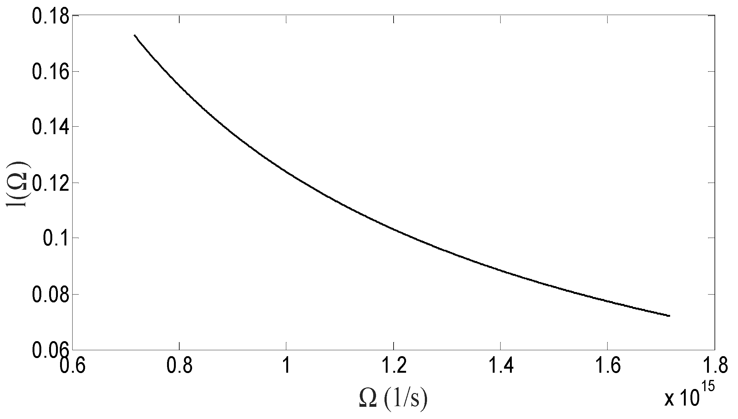
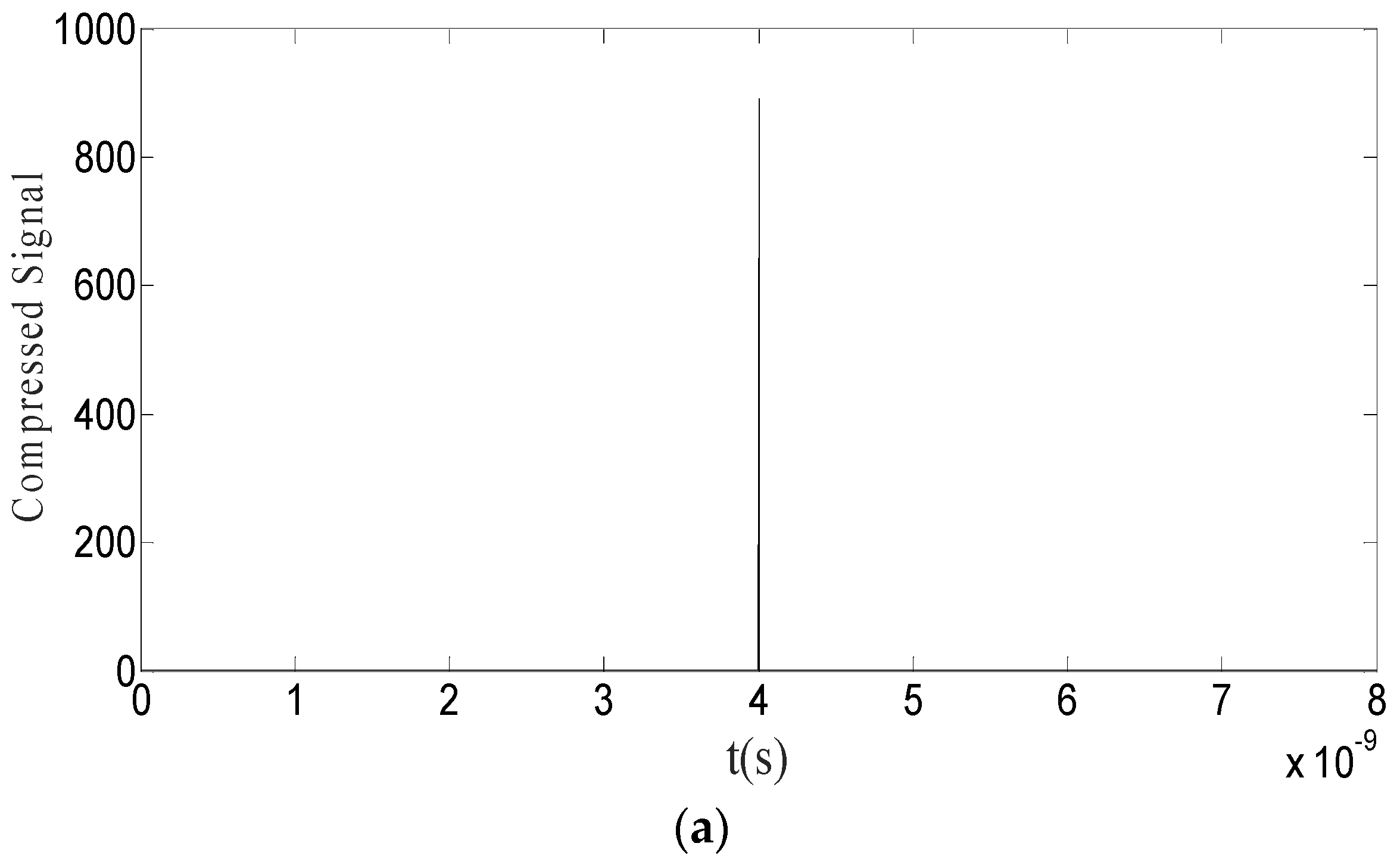
2.2. Pulse Compression

To compress the spectral broadened laser pulse, it was directed into a combination of four prisms divided into two identical parallel sets (P1-P2 and P1′-P2′), as shown in Figure 3. The corresponding prisms of the two sets were located at the same x-positions and displaced in the y-axis. The first set acted as a Fourier transformer and was responsible for separating the frequency components comprising the pulse into parallel beams located at different y-positions. The second prism set acted as an inverse Fourier transformer and was responsible for the spatial overlap of the spectral components throughout the environment outside the compressor.

The frequency components comprising the pulse that was emitted from the first prism set were directed via 45° mirror M1 onto the cross section of a slab. The slab, which had a low absorption coefficient as well as a well-defined frequency-dependent Kerr coefficient, was sandwiched between two electrodes. To change the spectral optical paths, each location across the width of the slab was subjected to a DC electric field with a constant value and a variable length in y-axis. This was realized, as shown in Figure 4, by connecting one of the two electrodes to the ground and the other to a DC electric source. The latter electrode was made from a photo-conducting material and was homogeneously illuminated with an array of LEDs. To change the phases of the spectral components, a stretchable computer-controlled opaque screen was used to control the illuminated area across the width of the slab. The emitted radiation from the slab was redirected by the mirror M2 into the lower set of prisms. The location of M2 was arranged such that the spectral components intersected the third prism P2′ at the same locations with respect to the base from which they were emitted from the second prism P2 of the upper set. Due to the symmetry of the configuration, the spectral components were overlapped at the output edge of the fourth prism and had the same slope. The slab’s length was chosen so that the compressor would be approximately quadratic-shaped and the electric field across its thickness would have a moderate value. For all spectral components to be constructively superimposed at a desired location, the spectral phases had to be equal or shifted by multiple of $2\mathsf{\pi }$ at that location. As shown in Figure 3, to fulfill this condition, the spectral optical path lengths across the setup and outside it had to be determined without subjecting the slab to an electric field. By dividing each of the obtained spectral optical path lengths by its corresponding vacuum wavelength $\left(\mathsf{\lambda }\right)$ and ignoring the integer number, a dimensionless fraction of the spectral wavelength was obtained. The corresponding phase of this fraction was obtained as follows:

$$\mathsf{\phi }\left(\mathsf{\Omega }\right)=2\mathsf{\pi }\times \mathrm{Fraction}\left(\mathsf{\lambda }\right),$$

(18)

and the spectral angle $\Delta \mathsf{\phi }\left(\mathsf{\Omega }\right)$ for completing $\mathsf{\phi }\left(\mathsf{\Omega }\right)$ to $2\mathsf{\pi }$ was:

$$\Delta \mathsf{\phi }\left(\mathsf{\Omega }\right)=2\mathsf{\pi }-\mathsf{\phi }\left(\mathsf{\Omega }\right).$$

(19)

To account for $\Delta \mathsf{\phi }\left(\mathsf{\Omega }\right)$, as found in Equation (19), the nonlinear part of the refractive index of the slab’s material, given in Equation (1), was activated. This was realized by subjecting a particular length $\mathrm{l}\left(\mathsf{\Omega }\right)$ along the slab at the location corresponding to the frequency across the slab’s width to a DC electric field, according to:

$$\Delta \mathsf{\phi }\left(\mathsf{\Omega }\right)=\frac{2\mathsf{\pi }}{\mathsf{\lambda }}{\mathrm{n}}_2{\mathrm{E}}^2\mathrm{l}\left(\mathsf{\Omega }\right)$$

(20)

Solving Equation (20) for $\mathrm{l}\left(\mathsf{\Omega }\right)$, one obtains

$$\mathrm{l}\left(\mathsf{\Omega }\right)=\frac{\Delta \mathsf{\phi }\left(\mathsf{\Omega }\right)\mathsf{\lambda }}{2{\mathsf{\pi } \mathrm{n}}_2{\mathrm{E}}^2}=\frac{\Delta \mathsf{\phi }\left(\mathsf{\Omega }\right) \mathrm{c}}{{\mathsf{\Omega }\mathrm{n}}_2{\mathrm{E}}^2},$$

(21)

where ${\mathrm{n}}_2$ is the nonlinear Kerr coefficient of the slab’s material that was chosen to be the same as that of the fiber’s material,$\mathrm{l}\left(\mathsf{\Omega }\right)$ is the length along the slab corresponding to the frequency $\mathsf{\Omega }$ that was subjected to the DC electric field, and c is the vacuum velocity of light.

To simulate the temporal distribution resulting from the compressor at a desired location, an inverse fast Fourier transform (IFFT) algorithm was applied on the manipulated spectral phases.

2.2.1. Computations

The computation for determining $\mathrm{l}\left(\mathsf{\Omega }\right)$ given in (21) was performed for equilateral prisms of side length ${\mathrm{l}}_1$ = 0.22 m, height as h = 0.19 m, length between the end of the base of the first prism and the apex of the second one as ${\mathrm{l}}_2$ = 0.05 m, slab length as 0.2 m, slab thickness as 0.003 m, and electric field influencing the slab as 100 V/mm.

2.2.2. Results and Discussion

Figure 5 shows the fitted curve of the spectral length $\mathrm{l}\left(\mathsf{\Omega }\right)$ subjected to the DC electric field that influenced the slab to stimulate the frequency components to be in-phase at the desired location. The computation was carried out for a bandwidth of ${10}^{15}$ 1/s induced by modulating the pulsed laser phase by a frequency 1.2 GHz.

Figure 6 represents the compressed laser pulses computed for the modulating frequencies of 100 MHz and 1.2 GHz. For each of the modulating frequencies, the computation was performed for a fixed number of frequency samples $8\times {10}^6$. The results showed that the compression for the modulation frequency at 100 MHz was better than that found at 1.2 GHz. This behavior was due to the larger ratio of the selected frequencies relative to the actual frequencies at 100 MHz compared to that at 1.2 GHz. This may be attributed to the fact that 1.2 GHz were more under-sampled or strongly aliased. In practical application, all frequencies would be in-phase if the slab is subjected to the desired distribution of the electric field given by $\mathrm{l}\left(\mathsf{\Omega }\right)$. Therefore, in this case, it was suggested that much better compression would be achieved.

3. Conclusions

Although this proposal allowed an ordinary femtosecond laser to be generated, it differed from previous studies in the following respects. The pulses to be compressed were obtained from a mode-locked laser of moderate halfwidth and low power, such that self-phase-modulation could not be initiated. The compression was achieved using a one-stage compressor. The compressed pulses were generated at any desired location without the movement of the compressor elements. Moreover, from the above, it is evident that the spectral broadening of the laser pulse as well as the spectral phase manipulation depend only on ${\mathrm{n}}_2{\mathrm{E}}^2$ that must be in the order of ${\mathrm{n}}_0$. This condition can be easily achieved by the external variation of the electric field. Consequently, this model can be used for any frequency that is not markedly attenuated during propagation in the proposed setup.

References

1. Dey, D.; Tiwari, A.K. Controlling Chemical Reactions with Laser Pulses. ACS Omega 2020, 5, 17857–17867. [Google Scholar] [CrossRef] [PubMed]
2. Ikeda, K.; Kotaki, H.; Nakajima, K. X-ray generation by femtosecond laser pulses and its application to soft X-ray imaging microscope. AIP Conf. Proc. 2002, 634, 268–275. [Google Scholar] [CrossRef]
3. Afshari, M.; Krumey, P.; Menn, D.; Nicoul, M.; Brinks, F.; Tarasevitch, A.; Sokolowski-Tinten, K. Time-resolved diffraction with an optimized short pulse laser plasma X-ray source. Struct. Dyn. 2020, 7, 014301. [Google Scholar] [CrossRef]
4. Abbas, A.M.; Pan, Q.; Mandon, J.; Cristescu, S.M.; Harren Frans, J.M.; Khodabakhsh, A. Time-resolved mid-infrared dual-comb spectroscopy. Sci. Rep. 2019, 9, 17247. [Google Scholar] [CrossRef] [PubMed] [Green Version]
5. Borgwardt, M.; Omelchenko, S.T.; Favaro, M.; Plate, P.; Hohn, C.; Abou-Ras, D.; Schwarzburg, K.; van de Krol, R.; Atwater, H.A.; Lewis, N.S.; et al. Femtosecond time-resolved two-photon photoemission studies of ultrafast carrier relaxation in Cu2O photoelectrodes. Nat. Commun. 2019, 10, 2106. [Google Scholar] [CrossRef]
6. Subramaniam, T.K. Erbium Doped Fiber Lasers for Long Distance Communication Using Network of Fiber Optics. Am. J. Opt. Photonics 2015, 3, 34–37. [Google Scholar] [CrossRef]
7. Ono, M.; Hata, M.; Tsunekawa, M.; Nozaki, K.; Sumikura, H.; Chiba, H.; Notomi, M. Ultrafast and energy-efficient all-optical switching with graphene-loaded deep-subwavelength plasmonic waveguides. Nat. Photonics 2019, 14, 37–43. [Google Scholar] [CrossRef] [Green Version]
8. Mottay, E.; Liu, X.; Zhang, H.; Mazur, E.; Sanatinia, R.; Pfleging, W. Industrial applications of ultrafast laser processing. MRS Bull. 2016, 41, 984–992. [Google Scholar] [CrossRef]
9. Alio, J.L.; AAbdou, A.A.; Puente, A.A.; Zato, M.A.; Nagy, Z. Femtosecond Laser Cataract Surgery: Updates on Technologies and Outcomes. J. Refract. Surg. 2014, 30, 420–427. [Google Scholar] [CrossRef] [PubMed]
10. Karasawa, N.; Morita, R.; Shigekawa, H.; Yamashita, M. Generation of intense ultrabroadband optical pulses by induced phase modulation in an argon-filled single-mode hollow waveguide. Opt. Lett. 2000, 25, 183–185. [Google Scholar] [CrossRef] [Green Version]
11. Hanna, M.; Delen, X.; Lavenu, L.; Guichard, F.; Zaouter, Y.; Druon, F.; Georges, P. Nonlinear temporal compression in multipass cells: Theory. J. Opt. Soc. Am. 2017, 34, 1340–1347. [Google Scholar] [CrossRef]
12. Weidner, P.; Penzkofer, A. Spectral broadening of picosecond laser pulses in optical fibres. Opt. Quantum Electron. 1993, 25, 1–25. [Google Scholar] [CrossRef] [Green Version]
13. Lu, C.-H.; Witting, T.; Husakou, A.; Vrakking, M.; Kung, A.H.; Furch, F.J. Sub-4 fs laser pulses at high average power and high repetition rate from an all-solid-state setup. Opt. Express 2018, 26, 8941–8956. [Google Scholar] [CrossRef] [PubMed]
14. Saleh, M.F.; Biancalana, F. Soliton dynamics in gas-filled hollow-core photonic crystal fibers. J. Opt. 2016, 18, 013002. [Google Scholar] [CrossRef] [Green Version]
15. Schmidt, B.E.; Béjot, P.; Giguère, M.; Shiner, A.; Trallero, C.; Bisson, E.; Kasparian, J.; Wolf, J.-P.; Villeneuve, D.; Kieffer, J.-C.; et al. Compression of 1.8 μm laser pulses to sub two optical cycles with bulk material. Appl. Phys. Lett. 2010, 96, 121109. [Google Scholar] [CrossRef] [Green Version]
16. Vuong, L.T.; Lopez-Martens, R.B.; Hauri, C.P.; Ruchon, T.; L’Huillier, A.; Foster, M.A.; Gaeta, A.L. Optimal pulse compression via sequential filamentation. In Proceedings of the Quantum Electronics and Laser Science Conference, Baltimore, ML, USA, 6–11 May 2007; p. JWE1. [Google Scholar]
17. Liao, K.-H.; Chen, M.-Y.; Flecher, E.; Smirnov, V.I.; Glebov, L.B.; Galvanauskas, A. Large-aperture chirped volume Bragg grating based fiber CPA system. Opt. Express 2007, 15, 4876–4882. [Google Scholar] [CrossRef] [PubMed]
18. Chauhan, V.; Bowlan, P.; Cohen, J.; Trebino, R. Single-diffraction-grating and grism pulse compressors. Opt. Soc. Am. 2010, 27, 619–624. [Google Scholar] [CrossRef]
19. Akturk, S.; Gu, X.; Kimmel, M.; Trebino, R. Extremely simple single-prism ultrashort-pulse compressor. Opt. Express 2006, 14, 10101–10108. [Google Scholar] [CrossRef] [PubMed] [Green Version]
20. Dombi, P.; Yakovlev, V.S.; O’Kee, K.; Fuji, T.; Lezius, M.; Tempea, G. Pulse compression with time-domain optimized chirped mirrors. Opt. Express 2005, 13, 10888–10894. [Google Scholar] [CrossRef] [Green Version]
21. Schulte, J.; Sartorius, T.; Weitenberg, J.; Vernaleken, A.; Russbueldt, P. Nonlinear pulse compression in a multi-pass cell. Opt. Lett. 2016, 41, 4511–4514. [Google Scholar] [CrossRef] [PubMed]
22. Nada, Y.S.; El-azab, J.M.; Othman, H.A.; Mohamad, T.; Maize, S.M.A. Interaction between Self Phase Modulation and Positive Group Velocity Dispersion in PMMA Polymer for Simplified Thin Film Compressor of High-Intensity Ultrashort Laser Pulses. Nonlinear Opt. Quantum Opt. 2020, 52, 299–311. [Google Scholar]
23. Shank, C.V.; Fork, R.L.; Yen, R.; Stolen, R.H. Compression of femtosecond optical pulses. Appl. Phys. Lett. 1982, 40, 761–763. [Google Scholar] [CrossRef]
24. Nikolaus, B.; Grischkowsky, D. 12× pulse compression using optical fibers. Appl. Phys. Lett. 1982, 42, 117–121. [Google Scholar] [CrossRef]
25. Tomlinson, W.J.; Stolen, R.H.; Shank, C.V. Compression of optical pulses chirped by self-phase modulation in fibers. J. Opt. Soc. Am. B 1984, 1, 139–149. [Google Scholar] [CrossRef]
26. Mével, E.; Tcherbakoff, O.; Salin, F.; Constant, E. Extracavity compression technique for high-energy femtosecond pulses. J. Opt. Soc. Am. B 2003, 20, 105–108. [Google Scholar] [CrossRef]
27. Jiménez, M.A.B.; Kuzin, E.A.; Ibarra-Escamilla, B.; Flores-Rosas, A. Optimization of the two-stage single-pump erbium-doped fiber amplifier with high amplification for low frequency nanoscale pulses. Opt. Eng. 2007, 46, 125007. [Google Scholar] [CrossRef]
28. Quintela, M.A.; Quintela, C.; Lomer, M.; Madruga, F.J.; Conde, O.M.; Lopez-Higuera, J.M. Comparison between a symmetric bidirectional-pumping and a unidrectional-pumping configurations in an erbium fiber ring laser. Int. Soc. Opt. Eng. 2007, 6619, 440–443. [Google Scholar]
29. Milonni, P.W.; Eberly, J.H. Introduction to Nonlinear Optics, 2nd ed.; John Wiley Sons, Inc.: Hoboken, NJ, USA, 2010; Chapter 10. [Google Scholar]
30. Bronshtein, I.N.; Semendyayev, K.A.; Musiol, G.; Muehlig, H. Handbook of Mathematics, 5th ed.; Springer: Berlin/Heidelberg, Germany, 2007. [Google Scholar]
31. Qian, S.; Li, J.; Zhang, Y. Absorptive Nonlinearity in Er-Doped Optical Fiber. Wuhan Univ. J. Nat. Sci. 1999, 4, 175–178. [Google Scholar] [CrossRef]
32. Fleming, J.W.; Wood, D.L. Refractive index dispersion and related properties in fluorine doped silica. Appl. Opt. 1983, 22, 3102–3104. [Google Scholar] [CrossRef]
Figure 1. The modulus given in Au of the amplitude spectrum resulting from the (FFT) algorithm computed at Ze = 2 m for the electric-field amplitude of a laser pulse of input maximum power 1.8 W, duration of 1 × 10 7 s, and a modulating frequency of 1.2 GHz.
Photonics 09 00205 g001
Figure 2. The normalized amplitude of the phase−modulated laser pulse of maximum power 1.8 W, duration 1 × 10 7 s computed at the end of the fiber z = 10 m and a modulating frequency 1.2 GHz.
Photonics 09 00205 g002
Figure 3. Overview of the compressor setup P1, P2, P1′, and P2′ are four prisms, L is a pulsed laser, P is a pump source, C is a capacitor M1 and M2 are mirrors and S is a slab subjected to a DC electric field.
Photonics 09 00205 g003
Figure 4. Overview of cross-sections in the slab responsible for stimulating the spectral phases to be in phase at any desired location.
Photonics 09 00205 g004
Figure 5. The fitted curve of the slab’s length l ( Ω ) subjected to a DC electric-field distribution across the slab’s width to equalize the phases of the spectral components of the broadened laser pulse at any desired location considering a laser with a pulse duration of 10 7   s, maximum power of 1.8 W, and phase modulated with a frequency of 1.2 GHz.
Photonics 09 00205 g005
Figure 6. The compressed laser pulses for modulating frequencies (a) 100 MHz and (b) 1.2 GHz.
Photonics 09 00205 g006aPhotonics 09 00205 g006b
Publisher’s Note: MDPI stays neutral with regard to jurisdictional claims in published maps and institutional affiliations.