Abstract
Due to limited data transmission bandwidth and data storage space, it is challenging to perform fast-moving objects classification based on high-speed photography for a long duration. Here we propose a single-pixel classification method with deep learning for fast-moving objects. The scene image is modulated by orthogonal transform basis patterns, and the modulated light signal is detected by a single-pixel detector. Thanks to the property that the natural images are sparse in the orthogonal transform domain, we used a small number of basis patterns of discrete-sine-transform to obtain feature information for classification. The proposed neural network is designed to use single-pixel measurements as network input and trained by simulation single-pixel measurements based on the physics of the measuring scheme. Differential measuring can reduce the difference between simulation data and experiment data interfered by slowly varying noise. In order to improve the reliability of the classification results for fast-moving objects, we employed a measurement data rolling utilization approach for repeated classification. Long-duration classification of fast-moving handwritten digits that pass through the field of view successively is experimentally demonstrated, showing that the proposed method is superior to human vision in fast-moving digit classification. Our method enables a new way for fast-moving object classification and is expected to be widely implemented.
1. Introduction
Object classification is the fundament of scene understanding and one of the most basic problems in machine vision [1]. Recently, with the help of deep learning, image-based object classification has made great progress [2,3,4,5,6,7,8]. However, object classification still faces many challenges, such as fast-moving objects classification for long-duration. The reason is two-fold. On the one hand, images of fast-moving objects captured by a regular camera might suffer from motion blur. On the other hand, although a high-speed camera can reduce motion blur, it is hardly possible to use the camera for long-duration image acquisition, because massive image data brings great difficulties to storage, transfer, and analysis [9].
Actually, images are an intermediate in the process of object classification. The object classification methods rely on the feature information embedded in the images rather than the images themselves. It is therefore possible to achieve object classification in an image-free manner if object feature information can be obtained without image reconstruction. Inspired by single-pixel imaging [10,11,12,13,14,15], single-pixel object classification without image reconstruction has recently been explored [16,17,18,19,20,21]. In these reported methods, the object light field is modulated by using special patterns to obtain the feature information of objects for classification of static objects, such as Hadamard-transform basis patterns [16], discrete-cosine-transform basis patterns [17], random patterns [18], and optimized patterns [19,20]. The single-pixel object classification methods are data- and bandwidth-efficient, allowing long-duration classification. Our group realized the classification of moving handwritten digits, using the single-pixel object classification method through the learning structured light illumination [21].
It is well-known that deep learning always needs a large amount of data to train networks [22]. In some cases, it may be difficult or time-consuming to collect thousands of labeled data on experiments. If the physical process of experiment is well understood, it is possible to use only a small number of training examples even simulation examples to train networks. M. R. Kellman et al. proposed a physics-based design that was learned by only a small number of training examples and generalized well in the experimental setting [23]. F. Wang et al. demonstrated that a neural network for single-pixel imaging can be trained by using simulation data [24]. However, how to establish a simulation physical model that is insensitive to some uncertain factors, such as noise, is the key to ensure that the network trained by simulation data is effective in practical application.
In this paper, we propose a single-pixel classification method with deep learning for fast-moving objects. Based on the structured detection scheme, the proposed method uses a small number of discrete-sine-transform (DST) [25] basis patterns for feature information acquisition, because most energy of natural images is concentrated at the low-frequency band and the images exhibit strong sparsity in the DST domain [26]. A single-pixel detector is used to measure the light signals modulated by these patterns and then the single-pixel measurements are sent to a neural network for classification. The neural network is designed to use single-pixel measurements as network input and trained by simulation single-pixel measurements based on the physical process of the measuring scheme. A differential measuring approach [27,28] can reduce the difference between simulation data and experimental data caused by slowly varying noise. To improve the credibility of classification results, we designed a repeated measurement data rolling utilization approach to increase the number of tests. The proposed method was experimentally demonstrated in the classification of handwritten digits on a fast-rotating disk. The results show that our method enables fast-moving object classification of a high accuracy in a noisy scene, which can hardly be achieved by human vision.
2. Methods and System Architecture
2.1. The System Architecture
The optical configuration of the proposed method, which is a structured detection scheme in single-pixel imaging, is illustrated in Figure 1 [12]. Figure 1a shows the optical system. The target object is illuminated by a light source and then is imaged on the modulation array of a spatial light modulator (SLM) by an imaging lens. The SLM generates a small number of DST basis patterns to modulate the image of the object. The modulated light is collected by a lens and is measured by a single-pixel detector. The single-pixel measurements are fed to a trained neural network, which outputs the classification results. Figure 1b shows the experimental setup. We use a light-emitting diode (LED) to illuminate the target object, and the object is imaged on a digital micromirror device (DMD) through Lens 1. The DMD generates a series of DST basis patterns to modulate the image of objects. As for a proof-of-concept demonstration, we take handwritten digits as target objects. The digits are laser-engraved on acrylic boards (black background and hollowed-out digits). The digits are put on a disk, as shown in Figure 1c, which can be driven by a motor. Then a photodiode is used as a single-pixel detector to measure the reflected light from DMD collected by Lens 2. The single-pixel measurements are fed to the neural network as input. The digits are from the MNIST (Modified National Institute of Standards and Technology) handwritten digits database [29]. The database provides 60,000 training images and 10,000 test images, each of which is pixels.
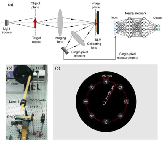
Figure 1.
Optical configuration of the proposed method: (a) optical system, (b) experimental setup, and (c) layout of the disk.
2.2. Differential Measuring in Transform Domain
An image contains rich information, but object classification needs only the specific feature information. In other words, the image data of objects are redundant for object classification. Just as the images and their DST spectra shown in Figure 2, most energy of natural images is concentrated at the low-frequency band, and the images exhibit strong sparsity in the DST domain. Therefore, it is possible to classify the target object with the low-frequency DST coefficients in a deep-learning manner, that is, achieving object classification by feeding the low-frequency DST coefficients to a trained neural network. Similar to Fourier single-pixel imaging [11], we use DST basis patterns to measure DST coefficients by a single-pixel detector, so as to avoid massive image data.
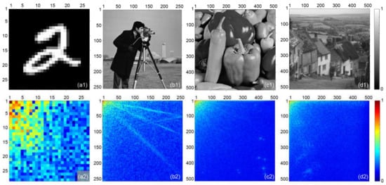
Figure 2.
Natural images and their DST spectra: (a1) handwritten digit “2” image ( pixels), (a2) DST spectrum of (a1), (b1) “Cameraman” image ( pixels), (b2) DST spectrum of (b1), (c1) “Peppers” image ( pixels), (c2) DST spectrum of (c1), (d1) “Goldhill” image ( pixels), and (d2) DST spectrum of (d1).
The discrete-sine-transform is expressed as follows:
where and are the coordinate in the spatial and transformation domain, respectively. Moreover, the inverse discrete-sine-transform is expressed as follows:
is the transformation kernel of DST, which is defined as follows:
In order to use a small number of the DST coefficients for training neural networks, we set quadrants with different radii as masks to select the coefficients from low-frequency to high-frequency in DST domain, as shown in Figure 3a. Figure 3b shows the examples of the selected low-frequency coefficients. The 8 masks have radii from 2 to 9 pixels, corresponding to 4, 9, 15, 22, 33, 43, 56, and 71 coefficients, respectively.
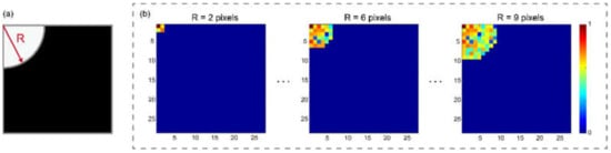
Figure 3.
Selection of DST coefficients: (a) a quadrant mask to select low-frequency coefficients and (b) selected low-frequency coefficients.
The DST basis patterns [25] we use can be expressed as follows:
where represents the basis patterns, and is a delta function expressed by the following:
We note that DMD can only generate non-negative intensity patterns, but, as Equations (1)–(5) imply, the intensity of the DST basis patterns contains negative value. Thus, we apply intensity normalization to the basis patterns, so that the intensity of the resulting patterns ranges from 0 to 1. The inversed patterns of can be obtained as . In addition, DMD is a binary device; hence, we utilize the “upsample-and-dither” strategy [30] for pattern binarization. The binarized basis patterns of the first four coefficients are shown in Figure 4.
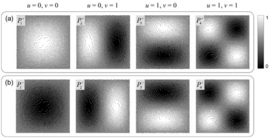
Figure 4.
Binarized basis patterns: (a) binarized basis patterns of the first four coefficients and (b) inversed patterns of (a).
By using the generated patterns to modulate the object image , the resulting single-pixel measurement is as follows:
We employ differential measuring in the acquisition of DST coefficients to reduce the difference between simulation data and experiment data caused by noise. We can acquire two single-pixel measurements and by a pair of DST basis patterns and , respectively. A differential single-pixel measurement is acquired by using the following calculation:
Specifically, each basis pattern displayed on the DMD is followed by its inversion . is exactly a DST coefficient. Thus, we acquire the 1D single-pixel measurements that is fed to a neural network for object classification.
2.3. Neural Network Design and Training
We designed a neural network that accepts single-pixel measurements as input to achieve object classification. The framework of the neural network is shown in Figure 5. It needs to be emphasized that the framework we chose is simple in order to preserve a high classification speed, although a sophisticated network framework may get better results. The neural network we employ consists of an input layer, a 1D convolution layer, three fully connected layers, and an output layer. The input layer has neurons, because the network is designed to accept measurements as input, that is, DST coefficients. There are 15 filters in the 1D convolution layer with kernel size of , and the three fully connected layers have 400, 200, and 100 units, respectively. There are neurons in the output layer for the classes. The nonlinear activation function rectified linear unit is used between fully connected layers, and the Softmax function is used in the output layer. In our proof-of-concept demonstration, equals 10. The output layer exports probabilities for classes. The class with maximum probability is picked as a classification result. The parameters in the network are initialized randomly with truncated normal distribution and then updated by the adaptive moment estimation (ADAM) optimization. The cross-entropy loss function is adopted for optimizing. The network is built on the TensorFlow version 2.1.0 platform, using Python 3.7.6.
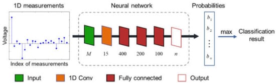
Figure 5.
Framework of the neural network.
Deep learning requires a large amount of data to train the network, but experimentally collecting tens of thousands of labeled data for the neural network training is time-consuming. To solve this problem, we generate simulation single-pixel measurements for network training based on the physical process of single-pixel measuring. The simulation single-pixel measurements are generated by calculating the inner products of the binarized basis patterns and a handwritten digit image, as shown in Figure 6. We apply the same procedure to each image in the MNIST database to generate simulation datasets. Note that, for non-differential mode, forms a non-differential dataset. For differential mode, the differences of and form a differential dataset.
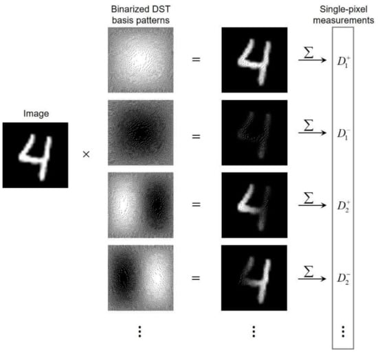
Figure 6.
Process of generating simulation data of single-pixel measurements.
Considering that the objects moving through the field of view have rotation, as shown in Figure 1, we rotate the handwritten digit images in the dataset with random angles. The center of the field of view is 112 pixels far from the center of disk point according to actual size. The digit images are randomly rotated between −4 and 4 degrees around point . Figure 7 shows the example of 5 pairs of original training images and the corresponding rotated images. The simulation single-pixel measurements for moving digits are generated by using the procedure shown in Figure 6.
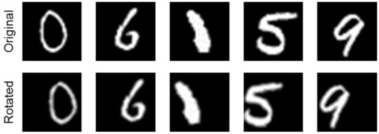
Figure 7.
Example of the training images. The first row shows the original images, and the second row shows the images with random rotation.
Therefore, according to the 8 groups of DST coefficients in Figure 3, we generate 4 kinds of simulation single-pixel measurement datasets for every group of coefficients. They are non-differential and differential datasets of original digits, and non-differential and differential datasets of rotated digits. Each dataset corresponds to 60,000 digits for training and 10,000 digits for testing. These simulation datasets are used to train the network shown in Figure 5, respectively. Training is run for 70 epochs. It takes ~5 min on a computer (AMD Ryzen 7 1700X CPU, 32-GB RAM, and an NVIDIA RTX 2080Ti GPU).
2.4. Data Rolling Utilization for Repeated Tests
In order to ensure the reliability of the classification results, we need to achieve repeated tests by taking full use of the acquired single-pixel measurements. This is because, from a statistical point of view, generally speaking, the more repeated tests, the higher reliability of the classification results. To achieve as many repeated tests as possible, we propose a data rolling utilization approach for repeated tests. Figure 8 shows the specific process of the proposed data rolling utilization approach for the differential mode.
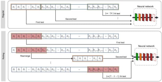
Figure 8.
Diagram of data rolling utilization approach for the differential mode.
We assume that, during the period that an object passes through the field of view, we obtain measurements for DST coefficients to perform a test; is an integer multiple of . For the differential mode, we assume that is the measurement for the first pattern , for the second pattern , and so on. Using Equation (7), we obtain differential measurements from the measurements. We can perform tests by using regular data utilization approach.
As for the data rolling utilization approach, we set a sliding window in a size of k, which slides 1 unit each time. The first window contains measurements from to , and we feed these measurements to the neural network for the first test. The second window contains measurements from to . Before the measurements contained in the second window are sent to the neural network, we rearrange the measurements into , , , , so that they follow the order from low-frequency to high-frequency in the DST domain. This is because and correspond to the same pattern. In this way, we can finally obtain tests from the measurements for differential mode. The proposed data rolling utilization approach significantly increases the number of tests by comparison with the regular data utilization approach.
The non-differential mode is similar to the differential mode. For the non-differential mode, we assume that is the measurement for the first pattern , for the second pattern , and so on. We can obtain only tests by using regular data utilization approach, but we obtain tests by using data rolling utilization approach from the measurements.
For continuous classification of moving objects, it is difficult to determine the time when the target object enters the field of view, so it is necessary to continuously measure the object in the field of view. Fortunately, single-pixel measurements produce much less data than image measurements. However, the faster the object moves, the fewer single-pixel measurements can be performed. Therefore, such a data rolling utilization approach is important in fast-moving object classification, as it improves the data utilization and increases the number of tests, enhancing the reliability of classification results.
3. Neural Network Performance Test
3.1. Network Performance Test with Simulation Data
Prior to the experiments, we evaluate the performance of the proposed network by using simulation test datasets, including original and rotated digit test datasets. We also evaluate the robustness of the proposed network by simulation test datasets with constant noise and slowly varying noise.
It is known that noise, such as slowly varying noise, is common in practical applications. Slowly varying noise usually comes from sunlight, lamplight, alternating-current power supply, and so on. The noise is slowly varying in comparison to the refresh rate of patterns. We assume that a simulation slowly varying noise is expressed as follows:
where the direct-current (DC) component, , represents the constant noise intensity; is the amplitude; is the frequency of the slowly varying noise; and is the refresh rate of patterns. Each pattern corresponds to a measurement. The moment of the -th measurement is . Equation (8) can be rewritten as follows:
We add to the simulation single-pixel measurements to generate noisy simulation test datasets. For the non-differential mode, the measurements are composed of , so the noisy measurements are expressed as follows:
forms the noisy test datasets for the non-differential mode.
For the differential mode, the noisy measurements are expressed as follows:
The noisy test dataset for the differential mode is generated by the differences of and :
Then we test the network trained by noise-free simulation datasets of original digits on the test datasets with slowly varying noise. The classification results are shown in Figure 9. For the noise expressed by Equation (8), we set the frequency, , of the slowly varying noise to 100 Hz (the power supply frequency), and the refresh rate, , of the pattern is 10,000 Hz. We set four values for the amplitude (0, 10, 20, and 30), which represents the effects of slowly varying noises. Then, for each , we set three values for the DC component, , which represents the effects of different constant noises. A noise-free condition is placed when (black line with triangle marker in Figure 9a). The mean voltage value of the simulation measurements is 52.72 V. According to the signal-to-noise ratio (SNR) formula , we calculate all the SNR with different DC components, . As shown in Table 1, the SNR is between 7.22 and −1.23 dB, which illustrates that the noise added to the simulation dataset seriously affects the acquired signal.
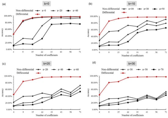
Figure 9.
Simulation classification accuracy of the original digit on noisy test sets with non-differential and differential mode: the amplitude of slowly varying noise (a) , (b) , (c) , and (d) .

Table 1.
DC component, , and corresponding SNR.
By combining Figure 9 and Table 1, we can draw the following conclusions. First, overall, the classification accuracy increases with the number of acquired coefficients. Second, for each amplitude, , the accuracy of the non-differential mode (black lines) decreases with the increase of DC component, , confirming that the network performance of the non-differential mode is seriously influenced by constant noise. Conversely, for each amplitude, , the accuracy of differential mode (red lines) maintains the same for different DC component, , so we represent the accuracy of differential mode by the same marker. It confirms that differential mode resists the influence of constant noise, because the constant noise is subtracted. Third, by comparing Figure 9a–d, we find that, with the increase of amplitude (), the accuracy of non-differential mode generally drops, while the accuracy of differential mode keeps at almost the same level. We thus confirm the robustness of differential mode against the slowly varying noise. When we employ 33 coefficients, the accuracy of differential mode has already reached 95.42%. Finally, we note that there is a trade-off between classification accuracy and measuring time. More coefficients mean high classification accuracy but a long measuring time. An appropriate number of coefficients should be chosen in terms of requirements.
Meanwhile, we also test the network trained by simulation datasets of rotated digits. We set as a noisy condition. The results are shown in Figure 10. By comparing them to the results of original digit datasets in Figure 9 in the same condition, the results of the rotated digit datasets give an average 9.04% decrease. Thus, it is indicated that the network has good robustness on rotated digits. Similar to the original image simulation results in Figure 9, we conclude that the non-differential mode is seriously influenced by noise, while the differential mode can reduce the impact of noise effectively. There is also a trade-off between classification accuracy and measuring time.
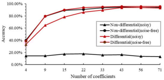
Figure 10.
Simulation classification accuracy of the rotated digit on noisy and noise-free test sets with non-differential and differential mode.
In summary, the test results of both simulation original and rotated datasets reveal that the differential mode has a remarkable performance in regard to noise immunity in slowly varying noise conditions.
3.2. Network Performance Test with Experiment Data of Static Objects
To confirm the generalization ability of the neural network and demonstrate that the network trained by simulation dataset can be applied in practical classification, we conduct experiments by using the setup shown in Figure 2b. A 10-watt white LED is used as a light source. The DMD (ViALUX V-7001), operating at its highest refreshing rate of 22,727 Hz, generates DST basis patterns. These DST basis patterns are scaled to pixels. A photodiode (Thorlabs PDA-100A2, gain = 0) is used as a single-pixel detector to collect the light reflected by the DMD. Moreover, a data acquisition card (National Instruments USB-6366 BNC) operating at 2 MHz is employed to digitalize the single-pixel measurements.
Considering the trade-off between classification accuracy and measuring time according to simulation results, we choose 9, 15, 22, and 33 coefficients to perform experiments. On the one hand, when the number of coefficients reaches nine, satisfactory classification accuracy can be obtained. On the other hand, using fewer coefficients guarantees a short measuring time.
In the static object experiment, the disk is stationary, and we randomly choose eight handwritten digits from the test set of the MNIST database as target objects. We use the network trained by simulation dataset of original images for classification. We select one of the digits to compare the simulation measurements and experiment measurements in Figure 11. For both non-differential mode and differential mode, the general trend of experiment measurements is similar to simulation measurements, meaning that the simulation data are close to the experiment data. However, for the non-differential mode, the average values of simulation data and experiment data are not exactly the same. As the dashed lines shown in Figure 11a,c, the normalized average value of simulation data and experiment data in non-differential mode is 0.5651 and 0.6461, respectively. For the differential mode, the average values of simulation data and experiment data are almost the same, i.e., 0.0224 in Figure 11b and 0.0461 in Figure 11d. According to the simulation results of Figure 9, the difference between the average value of the simulation data and experiment data affects the classification performance of non-differential mode, while the differential mode resists the influence of constant noise.
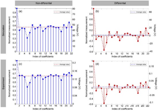
Figure 11.
Example of simulation single-pixel measurements and experiment single-pixel measurements.
The experiment classification results of static objects are shown in Table 2. We repeat the experiment many times for each chosen digit and present three groups of experiment results, that is, 24 tests for each number of coefficients under different conditions. Table 2 is the total number of correctly classified digits in the 24 tests.
Table 2.
Experiment classification results of 24 static digits.
The results of the noise-free condition demonstrate that, the more coefficients we use, the more digits can be correctly classified. Overall, the performance of differential mode surpasses that of non-differential. The classification results of differential mode are all correct, with more than 22 coefficients, while that of non-differential mode are all correct, with 33 coefficients.
To create a noisy experiment scene, we take a reading lamp as a noise source artificially. As shown in Figure 12, the noise, with a frequency of 100 Hz, is slowly varying compared to the refreshing rate of the DMD (22,727 Hz), which is consistent with that in simulation. The mean value of background noise is 0.086 V, as shown in Figure 12, and the mean value of desired signal is 0.13 V, as shown in Figure 11, so the SNR is 1.79 dB calculated by formula .
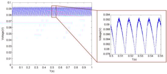
Figure 12.
Measurements of noise.
The results of the noisy experiment scene in Table 2 demonstrate that the classification performance of non-differential mode is affected by the noise, as the number of correct classifications in noisy condition is less than that in noise-free condition. Conversely, the results of the differential mode show that differential mode can reduce the impact of noise effectively. Overall, the performance of differential mode exceeds that of non-differential in either noisy or noise-free condition. The classification results of differential mode in both noisy condition and noise-free condition are all correct, with more than 22 coefficients.
The experiment results coincide with simulation results, thus confirming the feasibility of a network trained by simulation measurements applied to practical scenes. The method of training the network by simulation data removes the need of experimentally collecting massive labeled data; this is useful and may promote various deep learning fields.
3.3. Network Performance Test with Experiment Data of Moving Objects
We demonstrate the proposed method in classifying fast-moving digits by using the experimental setup shown in Figure 2b. The DMD, data acquisition card, and photodiode operate at the same parameters in static object experiments. We use the network trained by the simulation rotated image dataset for fast-moving object classification. The laser-engraved digits are put on a fast-moving disk that is driven by a motor. The disk can rotate at various speeds by tuning the Pulse-Width Modulation (PWM) of a speed controller. We set the PWM to 0%, 20%, 40%, and 60%, and the corresponding linear velocity of the digits is 0.729, 1.638, 4.265, and 6.626 m/s, respectively. These digits pass through the field of view successively. In order to show the speed of the fast-moving objects intuitively, we use a camera (FLIR, BFS-U3-04S2M-CS) of 60 fps to record videos of rotating digits at various speeds. The exposure time is 1/60 s and the frame of video is in a size of pixels. Figure 13 presents the snapshots of digit “4” in motion at various speeds (Visualization S1). The digit is moving so fast that it can hardly be recognized by the human eye even at the lowest linear velocity of 0.729 m/s.
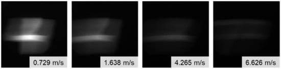
Figure 13.
Snapshots of digit “4” in motion at different speeds captured by using a 60-fps camera with an exposure time of 1/60 s (see Visualization S1).
As an example, we set PWM to 0% so that the digits move at a linear velocity of 0.729 m/s. Figure 14a shows the single-pixel measurements of the digits passing through the field of view successively in 1.5 s. We collect 34,090 single-pixel measurements. When the digits are moving in the field of view, light can pass through the disk, resulting in high intensity. Conversely, when there is no digit or the digit is partly in the field of view, the light is blocked by the disk, resulting in low intensity. We deliberately block one of the digits on the disk to mark the handwritten digits, such as the digit “2” shown in Figure 1c. Compared with the unblocked digits, there are more low-intensity measurements caused by the blocked digit. In this way, we can know which digit the intensity data correspond to. Figure 14b is the enlarged view of the single-pixel measurements of digit “4” in Figure 14a. Figure 14c is the differential measurements by using the measurements of Figure 14b based on Equation (7). During the period of an object passing the field of view, we can loop the DST patterns many times and acquire a series of single-pixel measurements, which are used to perform tests for a digit many times.
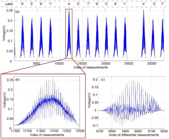
Figure 14.
Single-pixel measurements of moving digits: (a) single-pixel measurements of objects passing through the field of view successively in 1.5 s, (b) partially enlarged view of (a) (see Visualization S2), and (c) differential measurement from (b).
Only the entire digit in the field of view can be correctly classified, so we select the desired data by discarding measurements under the threshold. The threshold is computed by using the following calculation:
where represents the maximum of the single-pixel measurements, and the minimum. is a factor that controls the level of the threshold, which needs to be selected according to different experimental conditions. may be diverse at different speeds. The single-pixel measurements of the inversion pattern are usually low, so we select the desired data only by the single-pixel measurements of . Among the single-pixel measurements of , we look for the data continuously higher than the threshold, and these data are exactly the single-pixel measurements selected by the threshold.
We note that the faster objects move, the shorter time an object passes through the field of view, and the fewer measurements we acquire for an object. This results in a small number of tests. In practice, classification results are influenced by many factors, such as ambient noise. A small number of tests is highly contingent, hurting the reliability of classification results. Therefore, we propose the data rolling utilization approach in Section 2.4 to increase the number of tests, so as to improve the reliability of classification results.
The single-pixel measurements in Figure 14 are acquired with 15 coefficients in differential mode; that is, 30 measurements are employed for a classification test. By setting a threshold, we get 673 desired measurements from the single-pixel measurements in Figure 14b. If we adopt the regular data utilization approach, one test is conducted with every 30 measurements, so we can perform only 22 tests. If we adopt the data rolling utilization approach in Section 2.4, we can perform 322 tests with the same 673 desired measurements. The 322 test results are shown in Table 3. The digit “4” appears the most from the test results, so we regard it as the classification test result of the data in Figure 14b. If the test result is the same as the digit label, then the classification test is correct. In this way, we can get the classification results of other measurements.
Table 3.
Experiment test results of moving digits in Figure 14b.
We also take the reading lamp as a noise source (the noise is shown in Figure 12) and conduct four groups of comparative experiments with four linear velocities of the digits, 0.729, 1.638, 4.265, and 6.626 m/s. The experiment results are shown in Table 4. The following conclusions can be drawn. First, for all the four linear velocities, the results of non-differential mode are affected by noise seriously, as the correct/total in noisy condition drops dramatically versus that in noise-free condition. Second, as expected, when noise is added, the differential mode significantly outperforms the non-differential mode, which agrees with the simulation results shown in Figure 10. Third, when the digits move at low velocity, the correct/total improves with the number of coefficients on the whole. At 0.729 m/s, the correct/total of differential mode in noise-free condition achieves 100% with more than 15 coefficients. At 1.638 m/s, the correct/total of differential mode in noise-free condition achieves 100% with 22 coefficients. Finally, there is a trade-off between motion speed and the number of patterns. At both 4.265 and 6.626 m/s, differential mode performs the best with 15 coefficients, that is, 30 patterns, while non-differential mode performs the best with 22 coefficients, that is, 22 patterns. This is because more patterns take a longer time to acquire measurements for one classification, meaning severer motion blur.
Table 4.
Experiment classification results of moving digits.
4. Discussions
The target object we chose as a demonstration is pixels in size, totaling 784 pixels. In the experiment test, we, at most, selected 33 coefficients continuously from low-frequency to high-frequency in DST domain. According to the experiment results in Section 3.3, the trade-off between motion speed and the number of measurements indicates that more measurements decrease the accuracy when the object moves fast. On the premise of a favorable accuracy, we tend to use fewer coefficients. In the case of larger object image, such as pixels, the total pixels increase manifold. To keep a small number of measurements, the way to pick coefficients in transform domain is explored. Picking coefficients at intervals in the transform domain is a probable way.
It is thought that the classification ability of deep learning relies on the distribution of training data. If the distribution of training data is too far from the actual application, the classification ability of the network may decrease. In our experiment, the training data were designed in the definite application scene, moving digits on a rotating disk, which can hardly be adapted to objects with other movements.
The proposed method focuses on the classification scenes where the field of view contains only a single object. At the present stage, multiple objects classification is a more complicated problem, and our method does not apply to it. Improvement on feature acquisition and advanced network framework are expected to address the problems.
A camera acquires images directly, which we regard as measuring in “spatial domain”, whereas the proposed method measures in “transform domain”. The two measuring methods produce the same amount of data, but the measurement of each point of the two methods contains quite different information. A measurement in the transform domain corresponds to the weight of a frequency component in the spatial domain, which is the global information of spatial domain. However, a measurement in the spatial domain corresponds to only a pixel, which is the local information of the spatial domain. Performing classification by global information has an advantage over local information and is less disturbed by noise. In addition, the energy of natural images is concentrated at the low-frequency band in the transform domain; thus, we can carry out classification by a small number of measurements at the low-frequency band. Conversely, a small number of measurements in the spatial domain make it difficult to achieve object classification.
5. Conclusions
We proposed a single-pixel classification method with deep learning for fast-moving objects. Based on the structured detection scheme, the proposed method utilizes a small number of DST basis patterns to modulate the image of objects and acquires 1D single-pixel measurements sent to a neural network for classification. The neural network is designed to use differential measurements as network input and trained by simulation single-pixel measurements based on the physics of the measuring scheme. The differential measuring scheme can reduce the influence of slowly varying noise. Experiment results of rotating handwritten digits confirm that the neural network trained by simulation data has strong generalization ability. In order to ensure the credibility of moving-object classifications results, the data rolling utilization approach is employed for repeated tests. The correct/total of static object classification experiment reaches 100%. Meanwhile, the correct/total can reach 100% at low speed (0.727 and 1.638 m/s) and 74.84% when objects move as fast as 6.626 m/s. The motion speed of the object is limited by the refresh rate of the SLM. When noise is added, the differential mode significantly outperforms the non-differential mode. In the static object experiment, the correct/total of the differential mode improves by 58.13%, on average, over the non-differential mode. In the moving-object experiment, the correct/total of the differential mode improves by 26.18%, on average, over the non-differential mode. The results show that our method enables fast-moving object classification of a high accuracy in a noisy scene, which can hardly be achieved by human vision. The proposed method provides a new way to classify fast-moving objects.
Supplementary Materials
The following supporting information can be downloaded at https://www.mdpi.com/article/10.3390/photonics9030202/s1. Visualization S1: Moving digits at different speeds captured by using a 60-fps camera. Visualization S2: Single-pixel measurements of the moving digit ‘4’.
Author Contributions
Conceptualization, J.Z., M.Y. and S.Z; validation, M.Y., S.Z., Z.Z., J.P. and Y.H.; writing, M.Y., S.Z., J.Z. and Y.H.; supervision, J.Z.; funding acquisition, M.Y., Z.Z., J.P. and J.Z. All authors have read and agreed to the published version of the manuscript.
Funding
This research was funded by National Natural Science Foundation of China (NSFC), grant numbers 61905098 and 61875074; Fundamental Research Funds for the Central Universities, grant number 11618307; Guangdong Basic and Applied Basic Research Foundation, grant numbers 2020A1515110392 and 2019A1515011151; and Talents Project of Scientific Research for Guangdong Polytechnic Normal University, grant number 2021SDKYA049.
Institutional Review Board Statement
Not applicable.
Informed Consent Statement
Not applicable.
Data Availability Statement
The data presented in this study are available upon reasonable request from the corresponding author.
Conflicts of Interest
The authors declare no conflict of interest.
References
- Marr, D. Vision: A Computational Investigation into the Human Representation and Processing of Visual Information; The MIT Press: Cambridge, UK, 2010. [Google Scholar]
- Rawat, W.; Wang, Z. Deep convolutional neural networks for image classification: A comprehensive review. Neural Comput. 2017, 29, 2352–2449. [Google Scholar] [CrossRef]
- Ciregan, D.; Meier, U.; Schmidhuber, J. Multi-column deep neural networks for image classification. In Proceedings of the 2012 IEEE Conference on Computer Vision and Pattern Recognition (CVPR), Providence, France, 16–21 June 2012. [Google Scholar]
- Sermanet, P.; LeCun, Y. Traffic sign recognition with multi-scale convolutional networks. In Proceedings of the 2011 International Joint Conference on Neural Networks (IJCNN), San Jose, CA, USA, 31 July–5 August 2011. [Google Scholar]
- Bruce, V.; Young, A. Understanding face recognition. Br. J. Psychol 1986, 77, 305–327. [Google Scholar] [CrossRef] [PubMed]
- Jiankang, D.; Jia, G.; Niannan, X.; Stefanos, Z. Arcface: Additive angular margin loss for deep face recognition. In Proceedings of the IEEE Conference on Computer Vision and Pattern Recognition (CVPR), Long Beach, CA, USA, 16–20 June 2019. [Google Scholar]
- Zhao, R.; Yan, R.; Chen, Z.; Mao, K.; Wang, P.; Gao, R.X. Deep learning and its applications to machine health monitoring. Mech. Syst. Signal. Process. 2019, 115, 213–237. [Google Scholar]
- Andreopoulos, A.; Tsotsos, J.K. 50 years of object recognition: Directions forward. Comput. Vis. Image Und. 2013, 117, 827–891. [Google Scholar] [CrossRef]
- Vollmer, M.; Möllmann, K.P. High speed and slow motion: The technology of modern high speed cameras. Phys. Educ. 2011, 46, 191–202. [Google Scholar] [CrossRef]
- Edgar, M.P.; Gibson, G.M.; Padgett, M.J. Principles and prospects for single-pixel imaging. Nat. Photonics 2019, 13, 13–20. [Google Scholar] [CrossRef]
- Zhang, Z.; Ma, X.; Zhong, J. Single-pixel imaging by means of Fourier spectrum acquisition. Nat. Commun. 2015, 6, 6225. [Google Scholar] [CrossRef] [Green Version]
- Gibson, G.M.; Johnson, S.D.; Padgett, M.J. Single-pixel imaging 12 years on: A review. Opt. Express 2020, 28, 28190–28208. [Google Scholar] [CrossRef]
- Sun, B.; Edgar, M.; Bowman, P.R.; Vittert, L.E.; Welsh, S.; Bowman, A.; Padgettet, M.J. 3D computational imaging with single-pixel detectors. Science 2013, 340, 844–847. [Google Scholar] [CrossRef] [Green Version]
- Sun, M.J.; Zhang, J.M. Single-pixel imaging and its application in three-dimensional reconstruction: A brief review. Sensors 2019, 19, 732. [Google Scholar] [CrossRef] [Green Version]
- Yao, M.; Cai, Z.; Qiu, X.; Li, S.; Peng, J.; Zhong, J. Full-color light-field microscopy via single-pixel imaging. Opt. Express 2020, 28, 6521–6536. [Google Scholar] [CrossRef]
- Carmona, P.L.; Traver, V.J.; Sánchez, J.S.; Tajahuerce, E. Online reconstruction-free single-pixel image classification. Image Vision Comput. 2019, 86, 28–37. [Google Scholar] [CrossRef]
- He, X.; Zhao, S.; Wang, L. Ghost Handwritten Digit Recognition based on Deep Learning. arXiv 2020, arXiv:2004.02068. [Google Scholar] [CrossRef]
- Rizvi, S.; Cao, J.; Hao, Q. High-speed image-free target detection and classification in single-pixel imaging. In Proceedings of the SPIE Future Sensing Technologies, Online, 9–13 November 2020. [Google Scholar]
- Fu, H.; Bian, L.; Zhang, J. Single-pixel sensing with optimal binarized modulation. Opt. Lett. 2020, 45, 3111–3114. [Google Scholar] [CrossRef]
- Jiao, S.; Feng, J.; Gao, Y.; Lei, T.; Xie, Z.; Yuan, X. Optical machine learning with incoherent light and a single-pixel detector. Opt. Lett. 2019, 44, 5186–5189. [Google Scholar] [CrossRef]
- Zhang, Z.; Li, X.; Zheng, S.; Yao, M.; Zheng, G.; Zhong, J. Image-free classification of fast-moving objects using “learned” structured illumination and single-pixel detection. Opt. Express 2020, 28, 13269–13278. [Google Scholar] [CrossRef]
- Alzubaidi, L.; Zhang, J.; Humaidi, A.J.; Dujaili, A.A.; Duan, Y.; Shamma, O.A.; Santamaría, J.; Fadhel, M.A.; Amidie, M.A.; Farhan, L. Review of deep learning: Concepts, CNN architectures, challenges, applications, future directions. J. Big Data 2021, 8, 53. [Google Scholar] [CrossRef]
- Kellman, M.R.; Bostan, E.; Repina, N.A.; Waller, L. Physics-based learned design: Optimized coded-illumination for quantitative phase imaging. IEEE Trans. Comput. Imaging 2019, 5, 344–353. [Google Scholar] [CrossRef] [Green Version]
- Wang, F.; Wang, H.; Wang, H.; Li, G.; Situ, G. Learning from simulation: An end-to-end deep-learning approach for computational ghost imaging. Opt. Express 2019, 27, 25560–25572. [Google Scholar] [CrossRef]
- Gonzales, R.C.; Woods, R.E. Digital Image Processing, 4th ed.; Pearson Global Edition: Edinburgh, UK, 2020. [Google Scholar]
- Aelterman, J.; Luong, H.Q.; Goossens, B.; Pižurica, A.; Philips, W. COMPASS: A joint framework for parallel imaging and compressive sensing in MRI. In Proceedings of the 2010 IEEE International Conference on Image Processing (ICIP), Hong Kong, 12–15 September 2010. [Google Scholar]
- Sun, B.; Edgar, M.; Bowman, P.R.; Vittert, L.E.; Welsh1, S.; Bowman, A.; Padgett, M.J. Differential computational ghost imaging. In Proceedings of the Computational Optical Sensing and Imaging, Arlington, TX, USA, 23–27 June 2013. [Google Scholar]
- Welsh, S.S.; Edgar, M.P.; Bowman, R.; Jonathan, P.; Sun, B.; Padgett, M.J. Fast full-color computational imaging with single-pixel detectors. Opt. Express 2013, 21, 23068–23074. [Google Scholar] [CrossRef]
- LeCun, Y.; Cortes, C.; Burges, C.J.C. The MNIST Database of Handwritten Digits. Available online: http://yann.lecun.com/exdb/mnist/ (accessed on 22 February 2022).
- Zhang, Z.; Wang, X.; Zheng, G.; Zhong, J. Fast Fourier single-pixel imaging via binary illumination. Sci. Rep. 2017, 7, 12029. [Google Scholar] [CrossRef] [PubMed]
Publisher’s Note: MDPI stays neutral with regard to jurisdictional claims in published maps and institutional affiliations. |
© 2022 by the authors. Licensee MDPI, Basel, Switzerland. This article is an open access article distributed under the terms and conditions of the Creative Commons Attribution (CC BY) license (https://creativecommons.org/licenses/by/4.0/).