Infrared Ocean Image Simulation Algorithm Based on Pierson–Moskowitz Spectrum and Bidirectional Reflectance Distribution Function

Abstract

Infrared ocean image simulation has been widely used in water-pollution prevention, meteorological observation and melting-ice monitoring. However, in actual remote sensing observation scenes, the simulation images provided by conventional algorithms are lacking sufficient wave details because the viewing angle and the scale of simulation images are simplex. In this paper, an infrared ocean image simulation algorithm based on the Pierson–Moskowitz spectrum and a bidirectional reflectance distribution function is proposed. First, a 3D model of ocean surface is set up based on Pierson–Moskowitz spectrum. Then, the imaging position is calculated by the pinhole camera imaging method, which describes how each point of the 3D model is mapping to the 2D image. Next, by using a bidirectional reflectance distribution function, the radiation intensity from every point of the ocean model to the camera is computed. Finally, we figure up the sum of the radiation intensity received by every point of the detector and obtain the infrared simulation ocean image by quantizing the radiation intensity sum to grayscale. The entropy of the simulation images is 2.725, which is, respectively, improved by 71.86% and 16.83% compared with two other algorithms. The Kullback–Leibler divergence of the simulation images is 11.446, which is improved by 0.54% and 0.59% compared with other algorithms. The quantitative experimental results prove that the authenticity and clarity of the presented simulation images have remarkable advantages over conventional algorithms.

1. Introduction

Infrared ocean image simulation algorithms play an important role in water-pollution prevention, meteorological observation and melting-ice monitoring. However, there are some technological difficulties in the conventional algorithms. First, in the remote sensing observation scene, the conventional algorithms cannot provide simulation images, which contain plenty wave details. Second, the viewing angle and scale of the simulation images are simplex. Therefore, the infrared ocean image simulation algorithm needs to be deeply studied.

There are two main types of simulation algorithms for infrared ocean images. One type of algorithm generated images by attaching wave texture information onto a 3D ocean model [1,2,3]. Wen et al. [1] obtained images by adapting a hardware based on shader techniques to add the texture maps to the 3D model constructed by the Pierson–Moskowitz spectrum (P-M spectrum). Shi et al. [2] used 2D FFT to fast compute the geometric model of the sea. They proposed a rendering technique based on a viewing point to accelerate infrared radiation computing. Wang et al. [3] presented a new description of the ocean model. The normal vectors of every element, instead of the coordinate positions, were adapted in the shader programming based on the graphic processing unit. Zhao et al. [4] calculated the sea surface through the P-M model to achieve the modeling and simulation of sea radiance outside the atmospheric layer. Tang et al. [5] proposed a method to obtain the law of the infrared-characteristic value under different weather parameters by a neural network. They reconstructed the infrared background of the ocean by combining the law of the infrared characteristic with weather parameters. Xiao et al. [6] established an infrared radiation characteristics simulation model of the sea surface and analyzed the influence of the environment. However, the camera factors were ignored in their works, which reduced the similarity between the imitation images and true images. The other type of algorithm generated infrared ocean images by creating a description of planar radiation intensity distribution and quantizing it to grayscale. Zhang et al. [7] set up the infrared radiation intensity model for the global ocean surface through the theory of heat transfer to obtain a global infrared ocean image. Chen et al. [8] calculated the emissivity, reflectivity and the bidirectional reflectance of the sea surface by comparing the theoretical data with the measured data. They applied the equivalent temperature method in the process of quantizing the radiation distribution into grayscale to obtain ocean images. Zhang et. al. [9] calculated the total infrared radiation of the JONSWAP-based 3D sea model. They simulated the ocean images by mapping the radiation to each pixel of the detector. Zhang et al. [10] realized the infrared imaging simulation process by combining the sea surface temperature distribution characteristics with the space coordinate transformation and projection mapping method. However, the radiance intensities influenced by the gradient of the ocean surface elements were ignored in their works. In conclusion, the existing methods are deficient in the authenticity of simulation images, mainly because: (1) the viewing angle and scale of the simulation images are simplex in the computing process; (2) the intensity of the reflected lightness, which is changed by the gradient of ocean waves, has not been considered. To solve the problem of lacking image authenticity and clarity, an infrared ocean image simulation algorithm based on the P-M spectrum and the bidirectional reflectance distribution function (BRDF) is proposed in this paper. First, we set up a 3D model of the ocean surface based on the P-M spectrum and divide the 3D ocean model into small elements. Then, the position of every element on the 2D image screen is computed based on the pinhole camera imaging method. Next, by using the BRDF, we calculate the radiation intensity from every element to the camera. In this step, the radiation intensity includes three parts: the ocean self-heating radiation, the reflection of the surface from the sun radiance, and the reflection from the sky background radiance. In addition, the radiation intensity from the atmosphere to the camera is also considered. Finally, the sum of the radiation intensity received by every pixel of the 2D image screen are counted and quantized to grayscale, and the infrared simulation image of the ocean can be thus obtained.

The main contributions of our study can be summarized as follows:

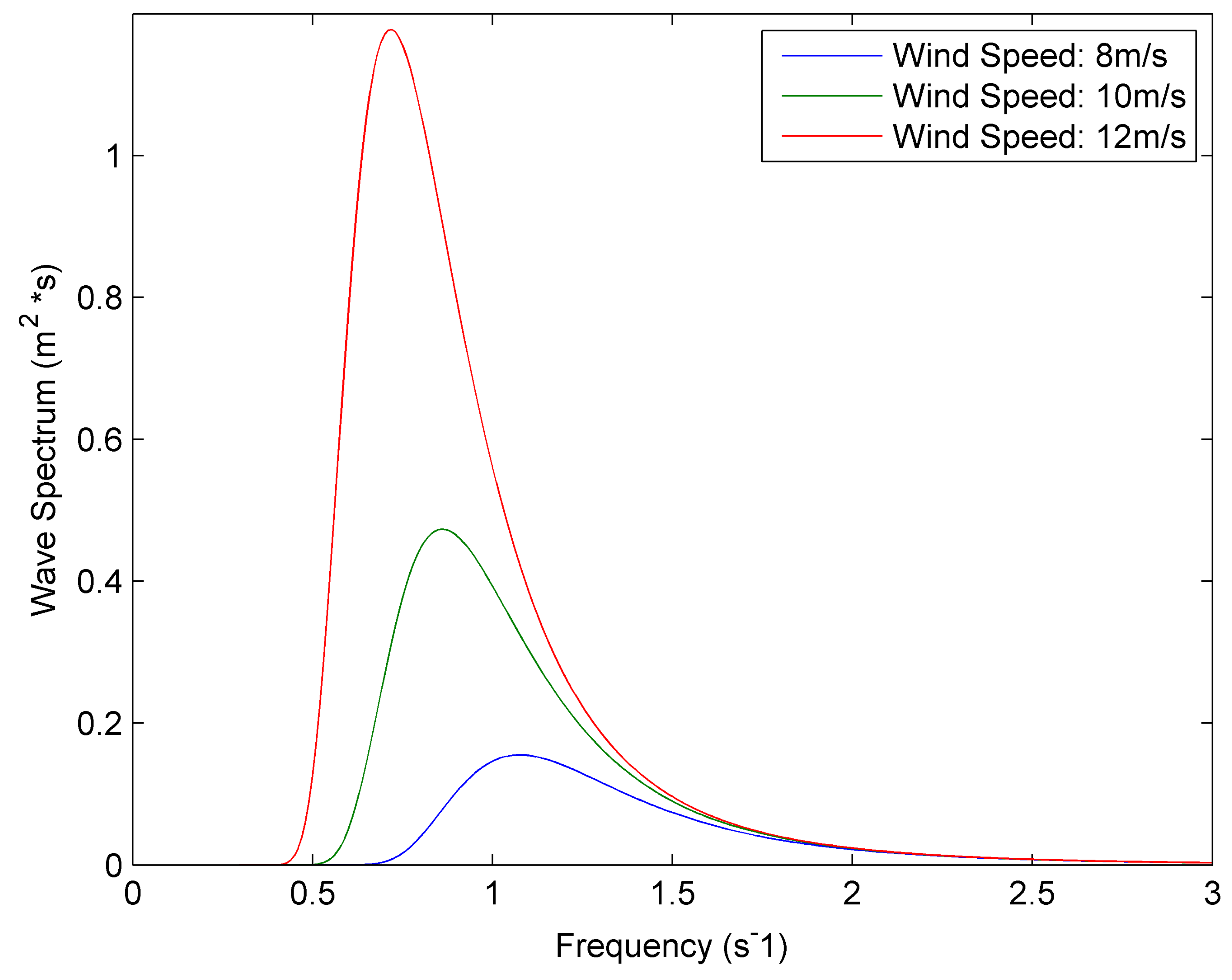
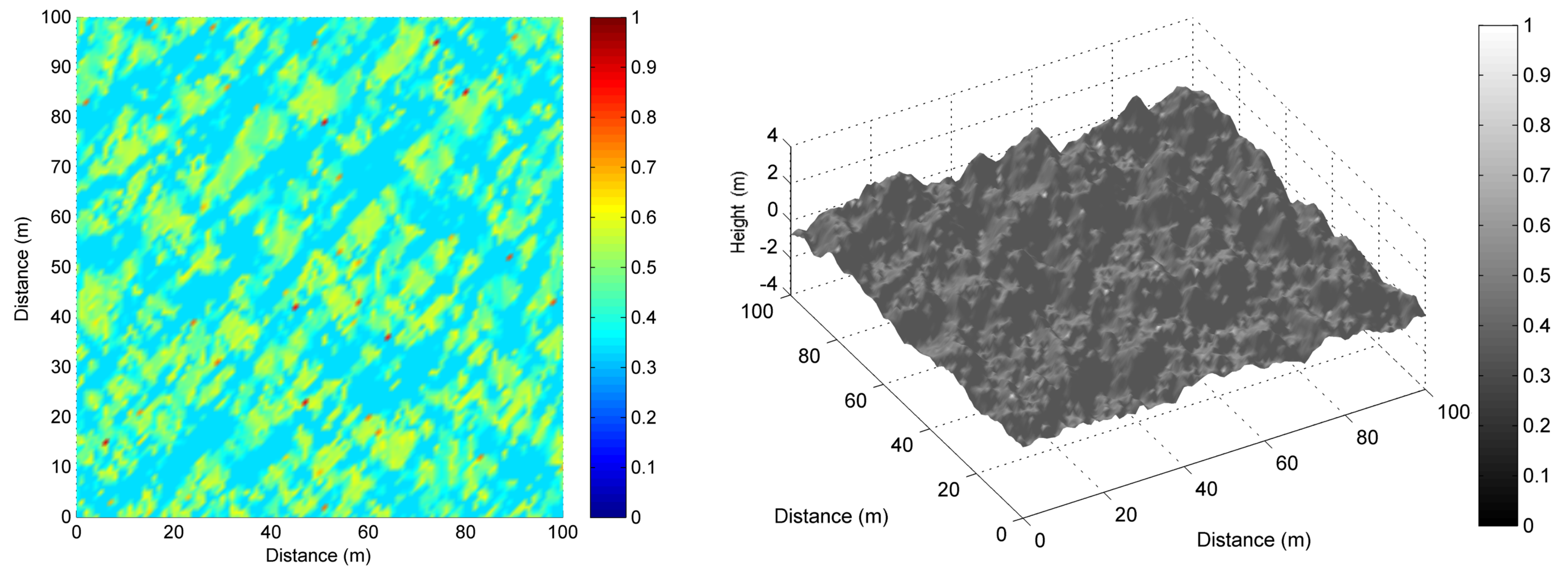
• Considering the deformation of the 3D ocean model caused by the changes of the camera shooting angle and distance, a position computing model combining the pinhole camera imaging process with a P-M spectrum-based 3D ocean model is proposed to improve the clarity of the simulation image. The influence of wave gradient changes is considered to help correct the model;
• To take into consideration the reflection of sun radiance and sky background radiance, we present a grayscale computing model based on the BRDF and pinhole camera imaging process to improve the authenticity of the simulation image. In addition, the scattered light in the atmosphere, which has direct influence on the image screen, is also considered in this model;
• A variety of infrared ocean simulation images under multiple camera shooting angles and spatial resolutions are provided. The clarity of the simulation image is quantitatively evaluated by the information entropy function. The authenticity of simulation images is quantitatively evaluated by the Kullback–Leibler divergence (K–L divergence).

This paper is organized as follows: Section 2 introduces the background of our study, from which our work is improved; in Section 3, the infrared ocean image simulation algorithm based on the P-M spectrum and the BRDF is introduced in detail; Section 4 discusses both the quantitative and qualitative experimental results; finally, a summary of this work is drawn in Section 5.

2. Background

In this section, we review a traditional 3D ocean model construction method and give a simulation example of it. The P-M spectrum, proposed by Pierson and Moskowitz, is a spectrum based on empirical observation. It is suitable for the fully grown sea surface. It represents the distribution of wave energy relative to wave frequencies. The formula of the P-M spectrum is [11]

$$S\left(w\right)=\frac{A{g}^2}{w^5}exp\left[-B{\left(\frac{g}{U_{19.5}w}\right)}^4\right].$$

(1)

where w is the frequency of the ocean waves, $A=8.1\times {10}^{-3}$, and $B=0.74$, $g=9.81$ m/s ${}^2$, and $U_{19.5}$ (m/s) is wind speed at 19.5 m above the ocean surface. Wind speed is the only variable parameter of the P-M spectrum. Figure 1 shows the wave spectrum distribution at different wind speeds.

The ocean surface can be regarded as the superposition of several wave functions with different frequencies, directions, amplitudes, and phase positions. The superimposed wave function represents the height of each point on the ocean surface. The linear superposition method is used to construct a 3D ocean model. The one-dimensional wave spectrum can be expressed as:

$$\xi \left(t\right)=\sum _{n=1}^{\infty }{a}_{n}cos\left(w_{n}t+{\epsilon }_n\right).$$

(2)

where $a_n$ is the amplitude, $w_n$ is the wave frequency, and ${\epsilon }_n$ represents the random phase position, which are uniformly distributed.

In actual application, the wave spectrum is expressed as:

$$\xi \left(t\right)=\sum _{n=1}^{\infty }\sqrt{2S\left(w\right)\delta w}cos\left(w_{n}t+{\epsilon }_n\right).$$

(3)

where $\delta w=w_n-w_{n-1}$ denotes the frequency interval. Equation (3) describes the frequency distribution of ocean energy.

The directional function recommended by the ITTC (International Towing Tank Conference) is expressed as:

$$\psi \left(w,\theta \right)=\psi \left(\theta \right)=\frac{2}{\pi }{cos}^2\left(\theta \right),-\frac{\pi }{2}<\theta <\frac{\pi }{2}.$$

(4)

where $\theta$ is the angle between wave direction and wind direction.

The distribution of direction $\theta$ is independent of the distribution of frequency w. The wave spectrum function, including the wave direction and wave frequency, is expressed as the product of two independent functions:

$$\begin{array}{ll}S\left(w,\theta \right)& =S\left(w\right)\psi \left(\theta \right)\\ & =\frac{\alpha g^2}{w^5}exp\left[-\beta {\left(\frac{g}{U_{19.5}w}\right)}^4\right]\times \frac{2}{\pi }{cos}^2\left(\theta \right).\end{array}$$

(5)

A wave surface $S\left({\omega }_i,{\theta }_i\right)$ can be constructed by (5), where the wave frequency ${\omega }_i$ and the wave direction $thet{a}_i$ have been determined. Multiple wave surfaces can be constructed by varying the value of $\omega$ and $\theta$. The 3D data of the ocean are the superposition of these wave surfaces. Theoretically, the range of wave frequency w is $\left(0,+\infty \right)$. It is not feasible to simulate the ocean surface through all the range of frequencies. As shown in Figure 1, there is a peak of the wave spectrum energy distribution. In practical cases, a segment around the peak, which includes more than 90% of the wave energy, is applied to simplify the computing process [12,13,14]. Then, the computing process can be simplified with little loss of image accuracy. By choosing the suitable value of frequency interval and direction interval, the 3D ocean model is obtained, as shown in Figure 2.

3. Theory of Infrared Ocean Image Simulation Algorithm

To improve the authenticity and clarity of the infrared ocean simulation image, we formulate a radiation construction model in this section. The proposed model works by calculating the composition of radiation received by the detector. It improves the image detail by splitting the ocean surface into tiny elements and computing the imaging position of them.

3.1. Reflection Model of Ocean Surface

The BRDF describes the relative amount of reflected radiation of incident irradiation. It includes both specular and diffuse reflectance components, expressed as [15]

$$F\left({\theta }_i,{\phi }_i,{\theta }_r,{\phi }_r,\lambda \right)=\frac{d{L}_r\left({\theta }_r,{\phi }_r,\lambda \right)}{d{E}_i\left({\theta }_i,{\phi }_i,\lambda \right)}.$$

(6)

where ${\theta }_i$ is the incident zenith angle, ${\theta }_r$ is the emergent zenith angle, ${\phi }_i$ is the incident orientation angle, ${\phi }_r$ is the emergent orientation angle, and $\lambda$ ($\mathsf{\mu }$ m) means the wavelength of incident light. In (6), $L_r\left(W/\left(m^2·sr·\mu m\right)\right)$ represents the radiance in the emergent direction and $E_i\left(W/m^2·\mu m\right)$ represents the irradiance in the incident direction. Figure 3 shows the physical model of the BRDF.

The high and low waves influenced by wind speed coexist in the ocean surface. By dividing the waves into tiny triangular elements with different normal directions, the reflected radiance can be easily calculated. Each element has three vertices A, B, and C. The normal direction of the element is calculated by the cross product of vector $\overrightarrow{AB}$ and $\overrightarrow{AC}$. By considering the positions of the sun and camera in the same coordinate system, the vector of the directions can also be calculated. Figure 4 shows the relationship between 3D ocean model and the reflection process on the elements of ocean surface.

As shown in Figure 4, L is the unit vector in the direction of the light source. N is the unit surface normal, H is the unit internal bisector of V and L, R is the unit vector in the reflection direction of the incident light, and V is the unit vector in the direction of the viewer. The surface element is not an ideal smooth surface. The facet slope distribution function is expressed as

$$D=\frac{exp\left(-{\left(tan\alpha /m\right)}^2\right)}{\pi m^2{cos}^4\alpha }.$$

(7)

where m is the root-mean-square slope of the facets; $\alpha$ is the intersection angle between N and H.

In this paper, the Cook–Torrance model is used to describe the BRDF, which can be expressed as [16]

$$F\left({\theta }_i,{\phi }_i,{\theta }_r,{\phi }_r,\lambda \right)=\frac{D·G}{4cos{\theta }_{i}cos{\theta }_r}.$$

(8)

where G represents the geometrical attenuation factor. In other words, G means the degree to which the small element is obscured from the incident light. The value of G is related to the direction of N, H, V, and L [16].

$L_r$ represents the reflection from the sea received by the detector. It includes the reflection of the sun and sky, which is transformed to the detector through the atmosphere. In the mid-wave infrared band, the reflection of the sky is negligible, so $L_r$ can be simply expressed as

$$L_r=\tau \left(\lambda \right)·F\left({\theta }_i,{\phi }_i,{\theta }_r,{\phi }_r,\lambda \right)·E_i\left({\theta }_i,{\phi }_i,\lambda \right).$$

(9)

where $E_i\left({\theta }_i,{\phi }_i,\lambda \right)$ is the incident solar spectral irradiance on the sea surface; $\tau \left(\lambda \right)$ is the atmospheric transmittance. $\tau \left(\lambda \right)$ is described in detail in Section 3.2.

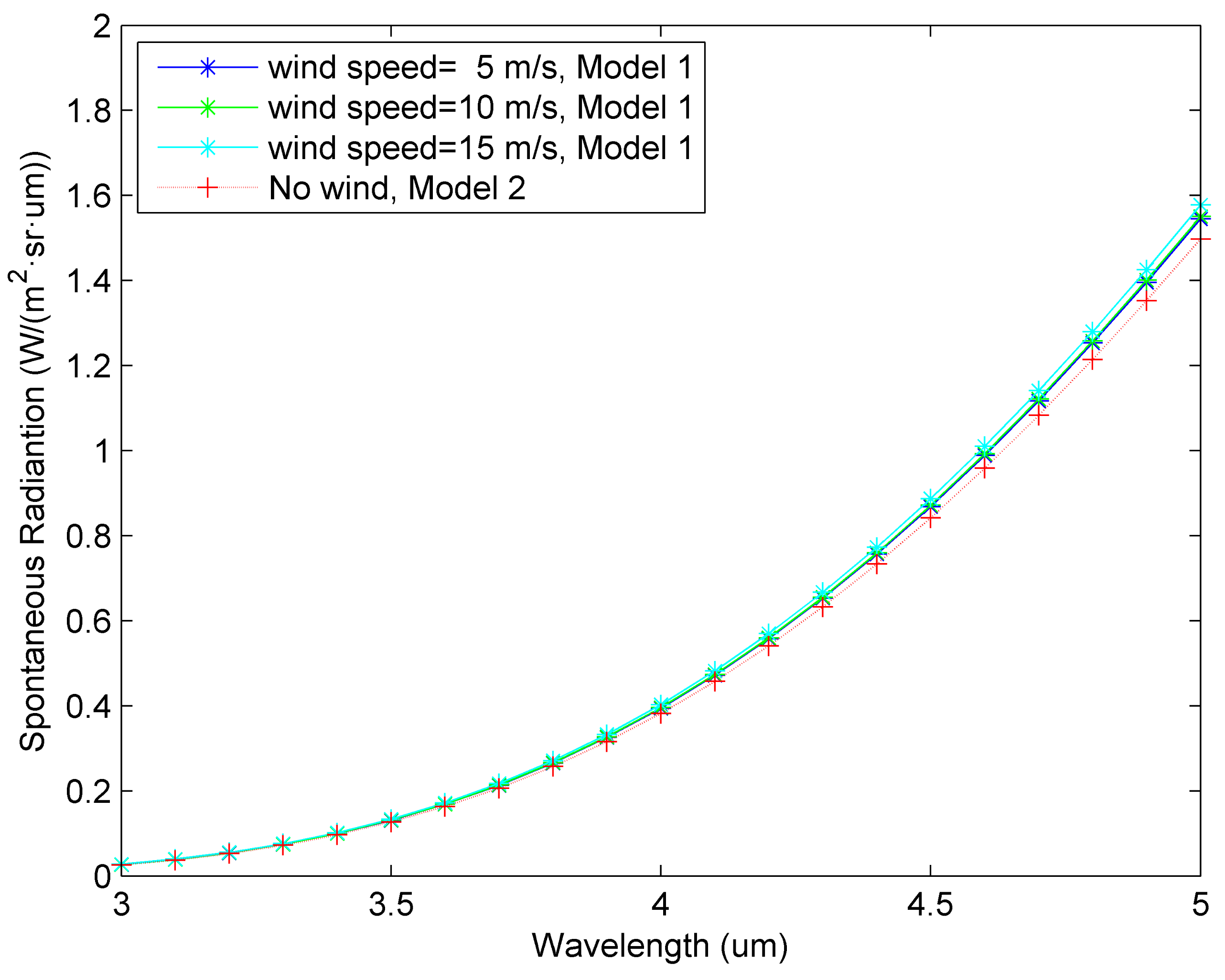
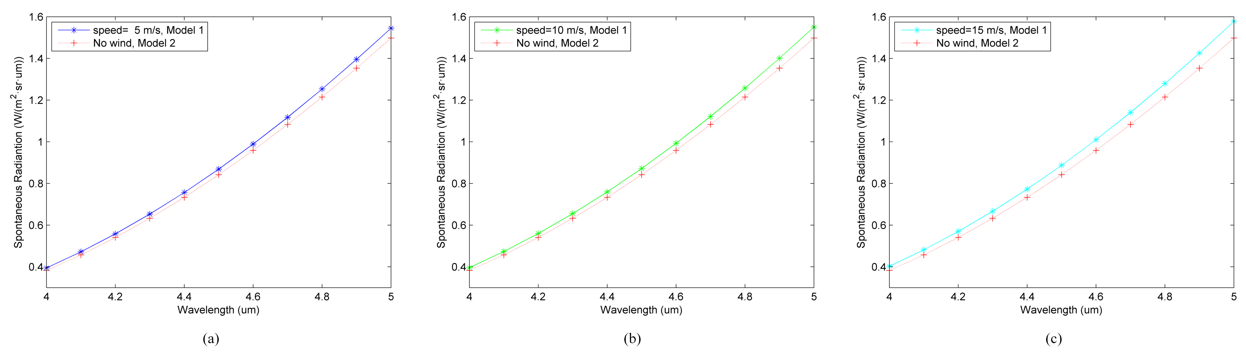
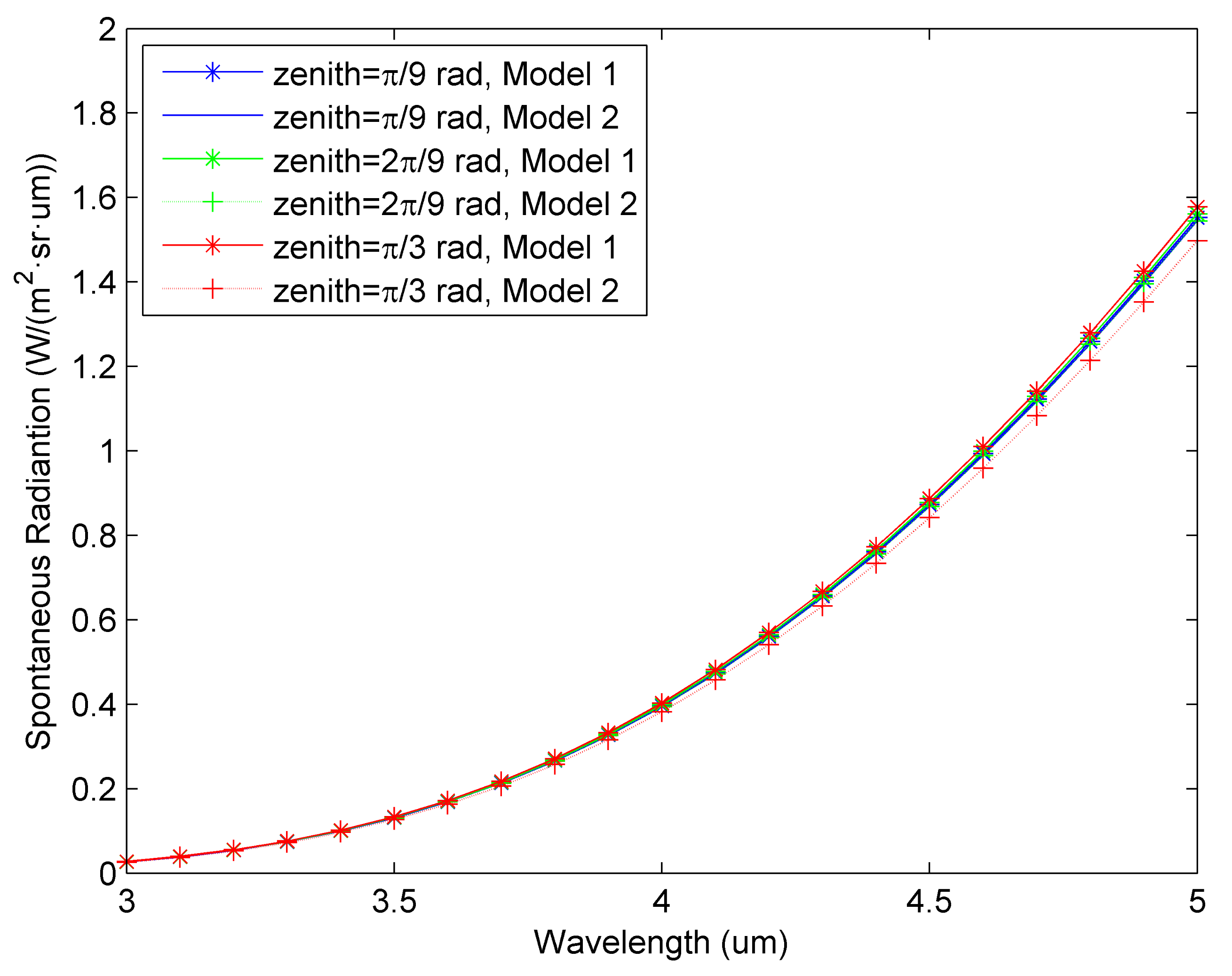
3.2. Spontaneous Radiation Model of Ocean Surface

The radiation received by detector $L_d$ consists of two parts: the reflection $L_r$ from the sea surface, and the spontaneous radiation $L_h$ from the sea.

$$L_d=L_r+L_h.$$

(10)

where the reflection $L_r$ has been introduced in Section 3.1 and $L_h$ describes the spontaneous radiation received by the detector.

$$L_h=\tau \left(\lambda \right)·{\epsilon }_{sea}·L_{BB}\left(\lambda ,T\right).$$

(11)

where ${\epsilon }_{sea}$ is the mean ocean surface emissivity, $L_{BB}\left(\lambda ,T\right)$ is the blackbody radiation at the same temperature with ocean, and $\tau \left(\lambda \right)$ is the atmospheric radiation transmittance.

If the detector is in the same aerosphere as the ocean surface, and there is almost no change of the atmospheric composition in the transmission path, the atmospheric transmittance $\tau \left(\lambda \right)$ can be described by the linear formula approximately, which is expressed as:

$$\tau \left(\lambda \right)=exp\left(-\left(a\left(\lambda \right)+b\left(\lambda \right)\right)\times L\right).$$

(12)

where $a\left(\lambda \right)$ is the attenuation coefficient of atmospheric absorption, $b\left(\lambda \right)$ is the attenuation coefficient of atmospheric scattering, and L means the transmission path length.

According to blackbody radiation law (Planck’s Law), the spectral emission of blackbody is

$$M_{\lambda bb}=\frac{c_1}{{\lambda }^5}·\frac{1}{exp\left(c_2/\lambda T\right)-1}.$$

(13)

where $c_1$ means the first radiation constant, and $c_2$ means the second radiation constant.

$$c_1=\left(3.7415\pm 0.0003\right)\times {10}^{8}W·{\mu m}^4·/m^2.$$

(14)

$$c_2=\left(1.43879\pm 0.00019\right)\times {10}^4\mu m·K.$$

(15)

Then we get the blackbody radiation

$$L_{BB}\left(\lambda ,T\right)=\frac{M_{\lambda bb}}{\pi }={\int }_{{\lambda }_1}^{{\lambda }_2}\frac{1}{\pi }\frac{c_1}{{\lambda }^5}·\frac{1}{exp\left(c_2/\lambda T\right)-1}d\lambda .$$

(16)

where ${\lambda }_1$ and ${\lambda }_2$, respectively, represent the lower and upper limit of the infrared wavelength range.

The atmospheric scattered light mainly occurs in the visible light band, so the atmospheric scattered light directly received by the infrared detector can be ignored.

3.3. Imaging Model of Ocean Surface

According to the above theoretical model, the radiation received by the detector, including the reflection from the sea surface and the spontaneous radiation of the sea, can be computed and quantized into grayscale. The radiation is focused on the detector’s photosensitive element, and is transformed into an electrical signal after electronic attenuation and photoelectric conversion. The electrical signal is expressed as,

$$V_s=L_{d\left(i,j\right)}\times R_d\times A_d.$$

(17)

$$L_{d\left(i,j\right)}=L_{r\left(i,j\right)}+L_{h\left(i,j\right)}+L_{s\left(i,j\right)}.$$

(18)

where $\left(i,j\right)$ denotes the position of the photosensitive element on the image plane, $R_d$ is the responsiveness of the detector, $A_d$ is the area of the photosensitive element, $L_{d\left(i,j\right)}$ is the infrared radiation illuminance received by the photosensitive element, and $L_{s\left(i,j\right)}$ represents the irradiation from the sky.

Then, the electrical signal is transformed into grayscale as follows,

$$f\left(i,j\right)=\frac{V_s-V_{min}}{V_{max}-V_{min}}·M.$$

(19)

where $V_{max}$ and $V_{min}$ represents the maximum and minimum electrical signal that a photosensitive element can output, M is the maximum grayscale, and $f\left(i,j\right)$ means the grayscale of the pixel on the image position $\left(i,j\right)$.

To obtain the infrared ocean simulation image, the projected position on the detector of each point on ocean surface is calculated by dividing the ocean surface into small elements. The suitable cutting size of the elements is chosen to improve the image clarity. The projected position of each element is computed by the pinhole camera imaging process as follows:

$$s\left[\begin{array}{c}u\\ v\\ 1\end{array}\right]=H\times \left[\begin{array}{cc}R& T\end{array}\right]\times \left[\begin{array}{c}\begin{array}{c}X\\ Y\end{array}\\ \begin{array}{c}Z\\ 1\end{array}\end{array}\right].$$

(20)

where s denotes the normalization coefficient, $\left[\begin{array}{c}u\\ v\end{array}\right]$ is the projected position of the center of an ocean element, H denotes the internal parameter matrix of the camera, R is the rotation matrix, T is the translation matrix, and $\left[\begin{array}{c}X\\ Y\\ Z\end{array}\right]$ represents the position of the element center in the world coordinate system. $\left[\begin{array}{cc}R& T\end{array}\right]$ can also be named as the external parameter matrix, which is related to the position of the detector and ocean. The internal matrix H is expressed as

$$H=\left[\begin{array}{ccc}f/D& 0& u_0\\ 0& f/D& v_0\\ 0& 0& 1\end{array}\right].$$

(21)

where f is the focal length, D represents the detector pixel size, and $u_0$ and $v_0$, respectively, denote half of the image length and width. The authenticity of the simulation image is improved by combining the reflection model, the spontaneous radiation model, and the pinhole camera imaging process. The clarity of the simulation image is improved by combining the pinhole camera imaging process with the method of constructing the 3D ocean model (in Section 2), with the influence of wave gradient changes considered in the algorithm.

According to the P-M spectrum, the 3D data of the ocean is constructed on square grids, whose sizes $S_{squ}$ can be changed. The ocean surface over one square grid can be divided into two triangular elements. When the camera focal distance, camera pixel size, and the observing distance have constant values, the spatial resolution is only determined by the size of the square grid. The spatial resolution of the image is closed to $n·S_{squ}$, where n represents the number of square grids observed by one pixel. The infrared ocean image simulation algorithm can provide a variety of images under multiple camera shooting angles and spatial resolutions.

4. Experimental Results

4.1. Analysis of Models

In order to verify whether the ocean spontaneous radiation in different observation zenith angles, at different wind speeds, and under different wavelengths conforms to the long-term experience in remote sensing observation, the spontaneous emission intensity received by the detector is calculated and compared with the computing result of the empirical formula in this section.

Figure 5 shows the spontaneous emission variation with wavelength at different zenith angles. The wind speed is 15 m/s and the observed zenith angles are, respectively, $\pi /9$, $2\pi /9$, and $\pi /3$ rad. The attenuation coefficient of atmospheric absorption and scattering is chosen to be 0.17, measured by Wang et al. [17]. The detection distance is 1 km.

The solid line is the value curve calculated according to the spontaneous radiation model in this paper (hereinafter referred to as Model 1). The dashed line is value curve calculated by the sea surface emission model presented by Wilson et al. [18] (hereinafter referred to as Model 2). In Model 2, ${\epsilon }_{sea}=0.98\left[1-{\left(1-cos\theta \right)}^5\right]$ is the mean ocean surface emissivity, where $\theta$ is the angle between the normal vector of ocean and the detecting direction. As shown in Figure 5, the radiation calculated by Model 1 and Model 2 under the same observed zenith angle share the similar trend of curve, but there is a slight difference in value. The difference of value curve can be seen more clearly in Figure 6.

As shown in Figure 6, the difference between the spontaneous radiation computed by Model 1 and Model 2 increases with the augment of observing zenith angle under the same detection wavelength. Taking the case at 5 $\mathsf{\mu }$ m, when the detection zenith angle is $\pi /9$, $2\pi /9$, and $\pi /3$ rad, the spontaneous radiation calculated by Model 1 is, respectively, increased by 0.43%, 1.08%, and 5.37%, comparing with Model 2. It is because Model 1 calculates spontaneous radiation when there is steady wind above the sea, and Model 2 computes when there is no wind. The variation of wind has an effect on the ocean surface, which eventually leads to the change of spontaneous radiation. The effect of wind is consistent with the experience of infrared remote sensing observations and is also shown by Model 1.

Figure 7 shows the spontaneous emission variation at different wind speeds. The observed zenith angle is $\pi /3$ rad, and the wind speeds are, respectively, 5, 10, and 15 m/s. The solid line is value curve calculated according to Model 1. The dashed line is value curve calculated by Model 2.

As shown in Figure 7, the radiation calculated by Model 1 and Model 2 at the same wind speed share the similar trend of curve, but there exists a slight difference, which can be seen more clearly in Figure 8. The difference between the spontaneous radiation computed by Model 1 and Model 2 increases with the augment of wind speed at the same observed zenith angle. Furthermore, taking the case at 5 $\mathsf{\mu }$ m, when the wind speed is 5, 10, and 15 m/s, the spontaneous radiation calculated by Model 1 is, respectively, increased by 3.17%, 3.55%, and 5.37%, comparing with Model 2. It is because the faster wind increases the gradient of ocean surface, which is consistent with the observation experience.

4.2. Analysis of Simulation Images

In this section, several examples of infrared ocean simulation image are given. The images are constructed by combining the radiation calculation model proposed in Section 3 with the P-M-spectrum-based 3D ocean model in Section 2. The simulation images are compared with the conventional algorithms.

4.2.1. Details and Parameter Setting

All the codes in this work are implemented on a PC with Intel i7-9700 CPU and 32.0 GB RAM. The comparisons between the simulation images obtained by the method in this paper (hereinafter referred to as Algorithm 1), the simulation images constructed by Shi et al. [2] (hereinafter referred to as Algorithm 2), and the simulation images constructed by Chen et al. [8] (hereinafter referred to as Algorithm 3) are conducted in this section. In order to facilitate the comparison with Algorithm 2 and Algorithm 3, the image resolution was used as an experimental parameter instead of a detector position, focal length, and detector pixel size. The parameters for constructing 3D ocean model and light conditions in the ocean do not have influence on the clarity and authenticity of simulation images. In this paper, these parameters are shown in

Table 1. The simulation parameters for constructing ocean appearance model and light model.

Parameter	Value	Value
Wind speed	10	m/s
Near-earth atmosphere temperature	290	K
Solar zenith angle	$\pi /6$	rad
Solar azimuth angle	$\pi /4$	rad

. Algorithm 1 and 2 need to construct an 3D ocean model before simulating images, while Algorithm 3 uses real remote sensing images of ocean as the texture mapping, without constructing 3D ocean model. For the sake of comparison, the parameters in Table 1 are consistent with the parameters used in taking the real ocean image in Algorithm 3.

As shown in

Table 2. The variable simulation parameters for imaging of ocean.

Parameter	Value	Value
Wavelength	3 to 5	$\mathsf{\mu }$ m
Image resolution	0.5, 1, 2	m
Detector zenith angle	0, $\pi /12,\pi /6$	rad
Detector azimuth angle	0, $\pi /2,\pi$	rad

, the parameters of detector have influence on the clarity and authenticity of simulation images. It is because in the scene of infrared remote sensing, the ocean can be detected in the 3 to 5 $\mathsf{\mu }$ m atmospheric window, but can be hardly detected in the 8 to 14 $\mathsf{\mu }$ m atmospheric window. The spatial resolution of real ocean image of Algorithm 3 is 0.65 m, so the spatial resolution in Table 2 is selected to be similar to 0.65 m. Considering the possible tilt of the camera during air-to-sea exploration, several typical zenith angles of the detector are chosen. In the simulating experiments, although the change of detector azimuth angle has little influence on the clarity and authenticity of simulation images, several azimuth angles in Table 2 are used in the experiments to help enrich the comparison.

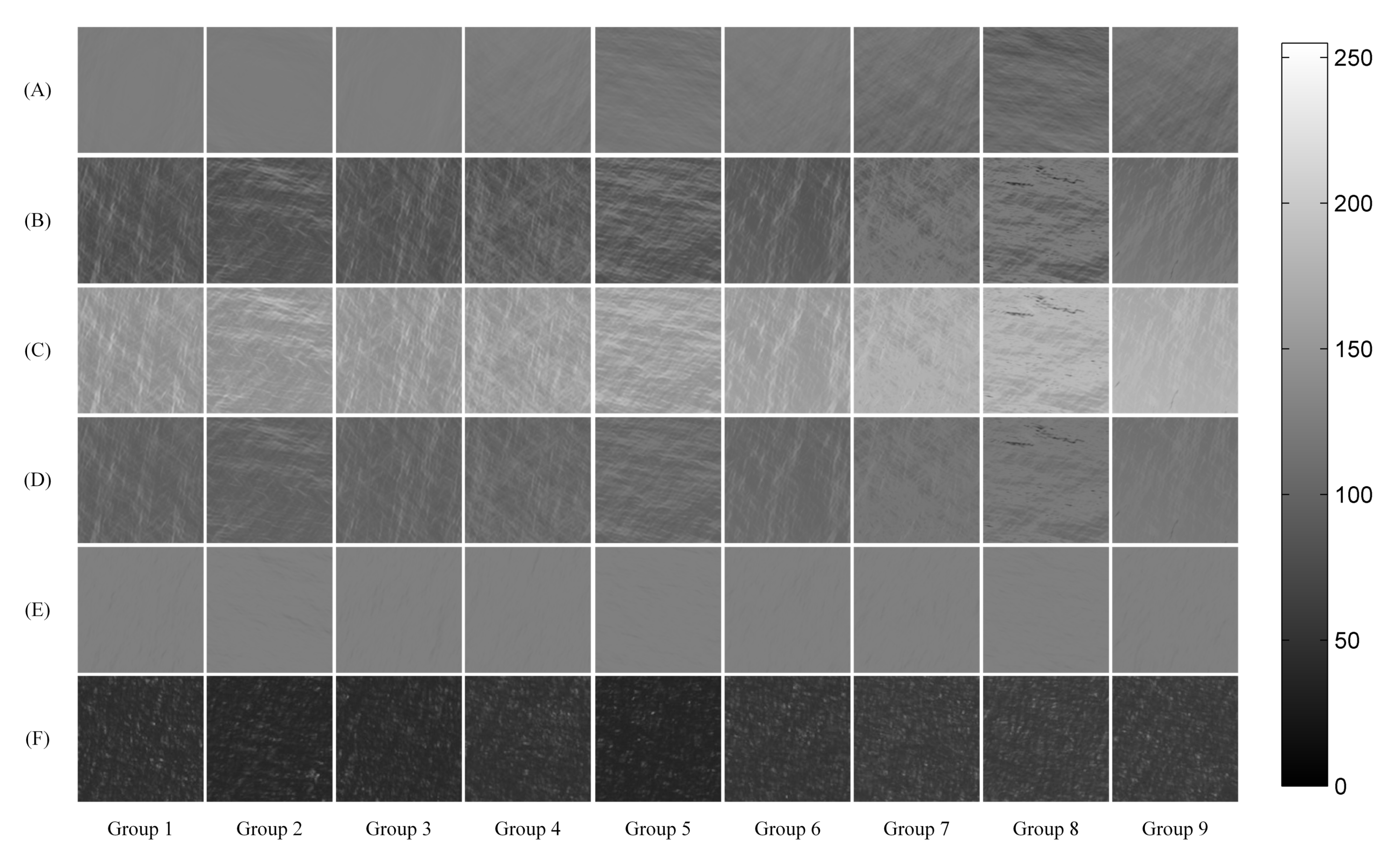
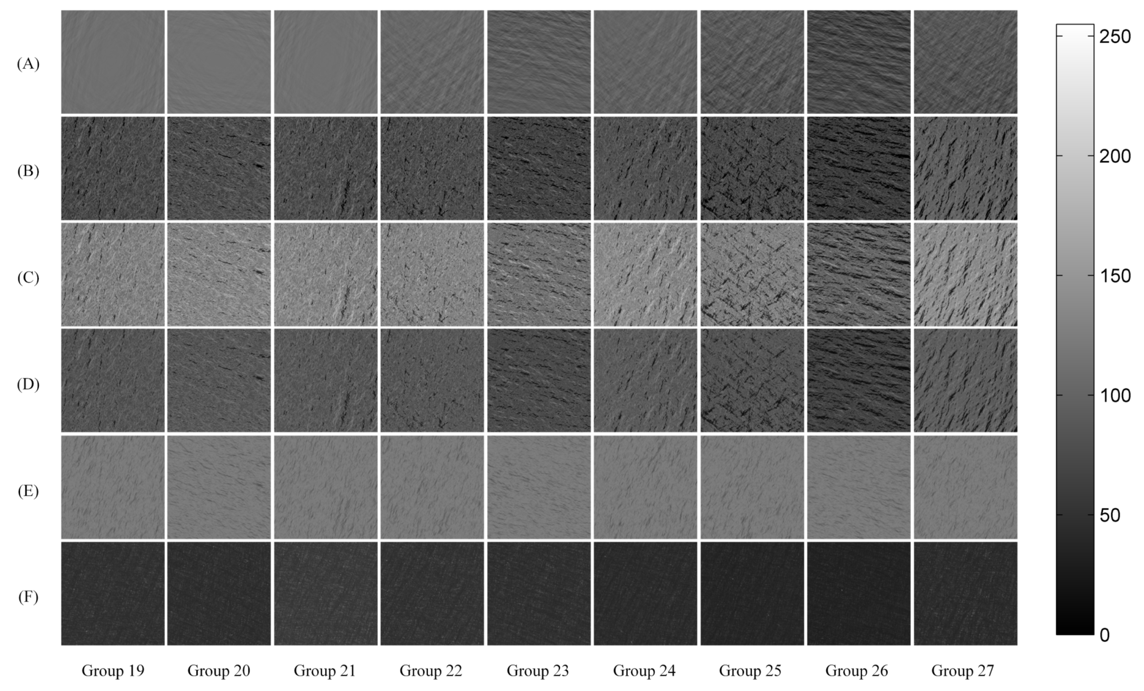
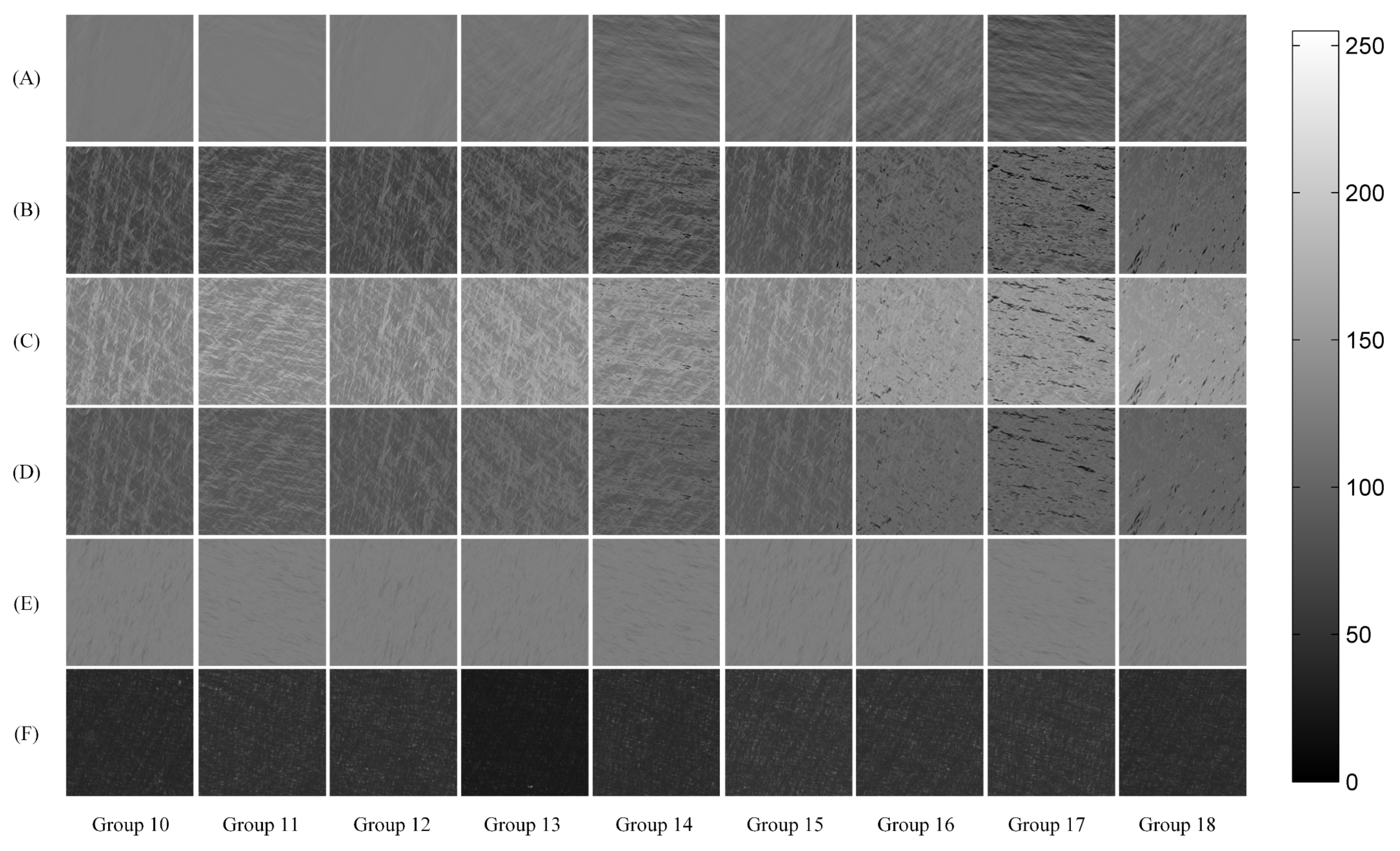
4.2.2. Qualitative Comparison

By permutation and combination of different parameter values in Table 2, we conducted 27 groups of experiments. The parameters of each group are shown in

Table 3. The detection parameters of experiments.

Group Number	Image Resolution/m	Detector Zenith Angle/rad	Detector Azimuth Angle/rad
1	0.5	0	0
2	0.5	0	$\pi /2$
3	0.5	0	$\pi$
4	0.5	$\pi /12$	0
5	0.5	$\pi /12$	$\pi /2$
6	0.5	$\pi /12$	$\pi$
7	0.5	$\pi /6$	0
8	0.5	$\pi /6$	$\pi /2$
9	0.5	$\pi /6$	$\pi$
10	1	0	0
11	1	0	$\pi /2$
12	1	0	$\pi$
13	1	$\pi /12$	0
14	1	$\pi /12$	$\pi /2$
15	1	$\pi /12$	$\pi$
16	1	$\pi /6$	0
17	1	$\pi /6$	$\pi /2$
18	1	$\pi /6$	$\pi$
19	2	0	0
20	2	0	$\pi /2$
21	2	0	$\pi$
22	2	$\pi /12$	0
23	2	$\pi /12$	$\pi /2$
24	2	$\pi /12$	$\pi$
25	2	$\pi /6$	0
26	2	$\pi /6$	$\pi /2$
27	2	$\pi /6$	$\pi$

. The results of all the experiments are shown in Figure 9, Figure 10 and Figure 11.

In each picture of Figure 9, Figure 10 and Figure 11, images in rows (A), (B), (C), and (D) show the images obtained by Algorithm 1. Images in row (A) show the spontaneous radiation images. Images in row (B) show the reflection intensity images. Row (C) shows the radiance map of the detector. Images in row (D) are the gray image of the detector, which are the simulation images obtained by Algorithm 1. In addition, images in row (E) are constructed by Algorithm 2. Images in row (F) are constructed by Algorithm 3. Images in the same group are constructed in the same condition. As shown in Figure 9, Figure 10 and Figure 11, the spontaneous radiation images in row (A) show little texture details, but can describe the temperature of ocean. The reflection intensity images in row (B) clearly display the texture detail, which denote the undulation of ocean. The radiance maps in row (C) are superimposed by images in row (A) and (B). Images in row (C) are transformed into images in row (D), which retain the information of column (A) and (B) without damaging many details.

Figure 9, Figure 10 and Figure 11, respectively, show the simulation images with the image resolution of 0.5 m, 1 m, and 2 m. The images obtained by Algorithm 1 have more texture details than Algorithm 2. With the increasing of resolution difference between real ocean image and simulation image, the clarity advantage of images constructed by Algorithm 1 is better than Algorithm 3. Groups 1, 4, and 7 in Figure 9, groups 10, 13, and 16 in Figure 10, and groups 19, 22, and 25 in Figure 11 share the same detector azimuth angle 0 rad, where the detector zenith angles are, respectively, 0 rad (groups 1, 10, and 19), $\pi /12$ rad (groups 4, 13, and 22), and $\pi /6$ rad (groups 7, 16, and 25). According to pictures in these groups, when the detector zenith angle is 0 rad, the texture details of images obtained by Algorithm 1 are similar to those from Algorithm 3, and are also similar to real ocean images. When the detector zenith angle is $\pi /12$ rad and $\pi /6$ rad, more stripes appear in the direction perpendicular to the camera moving path than in other directions. It is because the image compression in the camera movement leads to the stripes perpendicular to the camera. The simulation images constructed by Algorithm 1 can clearly show the change of stripes, while Algorithm 2 and 3 cannot show such details. The problem that the conventional algorithms are not so sensitive to the change of detection angle is solved by Algorithm 1.

4.2.3. Quantitative Comparison

Three parameters are used to evaluate the performance of the algorithm. The entropy function is used to calculate the clarity of image [19]. The K–L divergence is used to describe the similarity between simulation image and real ocean image, which explains the authenticity of simulation image [20]. The algorithm running time for single frame image is also counted to compare the algorithms.

The entropy function is expressed as [21]

$$D\left(f\right)=-\sum _{i=0}^{L-1}{p}_{i}ln\left(p_i\right).$$

(22)

where $p_i$ is the occurrence probability of pixels with grayscale i in the simulation image and L is the maximum gray level of the image. The clarity of image increases with the rise of the value of image entropy.

The K–L divergence is expressed as [20]

$$D_{KL}\left(p|q\right)=-\sum _{i=0}^{L-1}{p}_{i}ln\left(\frac{p_i}{q_i}\right).$$

(23)

where $q_i$ is the occurrence probability of pixels with grayscale i in the real image. The discrepancy between simulation images and real images decreases with the reduction of the absolute value of K–L divergence. The average evaluation index values of 27 groups of experiments are shown in

Table 4. Evaluation index of clarity and authenticity.

Evaluation Index	Algorithm 1	Algorithm 2	Algorithm 3
Entropy function	2.725	1.586	2.332
K–L divergence	11.446	11.508	11.514

. In addition, the average running time of all the experiments is shown in

Table 5. Running time of algorithms.

Evaluation Index	Algorithm 1	Algorithm 2	Algorithm 3
Running time/s	30.622	31.610	38.981

.

As shown in Table 4, compared with Algorithm 2 and 3, the clarity of images constructed by Algorithm 1 is, respectively, improved by 71.86% and 16.83%. The algorithm proposed in this paper has a significant improvement in image clarity. The average value of K–L divergence in Algorithm 1 is improved by 0.54% and 0.59% compared with Algorithm 2 and 3, which means the authenticity of images is better than conventional algorithms. As shown in Table 5, the running time of Algorithm 1 is reduced by 3.13% and 21.44% compared with Algorithm 2 and 3. In conclusion, compared with Algorithm 2 and 3, the authenticity and the clarity of the presented simulation images obtained by this paper have remarkable advantages.

5. Conclusions

In this paper, we propose an infrared ocean image simulation algorithm based on the P-M spectrum and BRDF. Firstly, a 3D ocean model is constructed by the P-M spectrum. Then, by using the pinhole camera imaging method, the imaging projection process is simulated to compute the position of the ocean elements on the image. Furthermore, the radiation intensity received by each pixel from each ocean element is calculated. Finally, we figure up the sum of the radiation intensity received by each pixel and obtain the simulation ocean image by quantizing the radiation intensity sum to grayscale. Both qualitative and quantitative experimental results prove that the authenticity and the clarity of the presented simulation images have remarkable advantages over the conventional algorithms.

The proposed algorithm can provide background image data for the traditional ocean target detection algorithm, so that the researchers can summarize the characteristics of the ocean image and construct new suppression methods of ocean image background. The algorithm can also quickly generate a large number of ocean images, which can provide training samples for the artificial intelligence algorithm of target detection in ocean scene. In addition, the proposed algorithm has some limitations. It is suitable for fully developed wind seas, but is unable to show the influence of ocean depth and seabed tilt. The algorithm used the BRDF, which is an empirical model based on measured data. It may lead to some errors with the real situation. Further research is needed for practical cases of ocean simulation in other occasions.

References

1. Wen, Z.; Liu, Z.; Liang, W. Real-time rendering of ocean special effects based on GPU. Comput. Eng. Des. 2010, 31, 4426–4429. (In Chinese) [Google Scholar]
2. Shi, K.; Hao, Y.; Wang, M.; Fu, S. Real-time simulation method of infrared sea background. Infrared Laser Eng. 2012, 41, 25–29. (In Chinese) [Google Scholar]
3. Wang, Y.; Xie, X.; Yang, J.; Fan, P. The Research on Dynamic Simulation of IR Sea Background Scene. J. Proj. Rocket. Missiles Guid. 2015, 35, 199–202, 207. (In Chinese) [Google Scholar]
4. Zhao, Y.; Li, Y.; Zhang, Y.; Rao, P. A space-based infrared detection scene generation system for moving objects with sea background. Opt. Precis. Eng. 2017, 25, 487–493. (In Chinese) [Google Scholar]
5. Tang, S.; Chen, Z.; Li, X. Study on Simulation of Sea Sky Infrared Imaging based on Neural Network and Measured Data. In Proceedings of the IOP Conference Series Materials Science and Engineering, Padang, Indonesia, 8–9 November 2018. [Google Scholar]
6. Xiao, C.; Lin, J.; Wu, K. Study on infrared radiation characteristics model of sea surface. In Proceedings of the Second Target Recognition and Artificial Intelligence Summit Forum, Shenyang, China, 28–30 August 2020. [Google Scholar]
7. Zhang, W.; Xuan, Y.; Han, Y. Infrared Image Simulation of Global Ocean Surface. Infrared Technol. 2006, 28, 170–173. (In Chinese) [Google Scholar]
8. Chen, X.; Lin, C.; Yang, L. Infrared Scene Simulation of Sea-Sky Background Based on Equivalent Temperature Method. Mech. Electr. Eng. Technol. 2015, 44, 36–39, 173. (In Chinese) [Google Scholar]
9. Zhang, X.; Wu, L.; Long, L.; Zhang, L. Detailed real-time infrared radiation simulation applied to the sea surface. In Proceedings of the International Conference on Optical Instruments and Technology, Beijing, China, 28–30 October 2017. [Google Scholar]
10. Zhang, H.; Qu, B.; Jin, L.; Ma, C. Infrared imaging simulation of sea surface detection of underwater vehicle thermal wake target. J. Appl. Opt. 2019, 40, 525–534. [Google Scholar]
11. Pierson, W.; Moskowitz, L. A proposed spectral form for fully developed wind seas based on the similarity theory of S. A. Kitaigorodskii. J. Geophys. Res. 1964, 69, 5181–5190. [Google Scholar] [CrossRef]
12. Chentanez, N.; Müller-Fischer, M. Real-time Eulerian water simulation using a restricted tall cell grid. ACM Trans. Graph. 2011, 30, 1–10. [Google Scholar] [CrossRef]
13. Wilf, I.; Manor, Y. Simulation of sea surface images in the infrared. Appl. Opt. 1984, 23, 3174–3180. [Google Scholar] [CrossRef] [PubMed]
14. Frechot, J. Realistic simulation of ocean surface using wave spectra. In Proceedings of the First International Conference on Computer Graphics Theory and Applications (GRAPP), Setúbal, Portugal, 25–28 February 2006. [Google Scholar]
15. Nicodemus, F. Directional Reflectance and Emissivity of an Opaque Surface. Appl. Opt. 1965, 4, 767–773. [Google Scholar] [CrossRef]
16. Cook, R.; Torrance, K. A reflectance models for computer graphics. ACM Trans. Graph. 1982, 1, 7–24. [Google Scholar] [CrossRef]
17. Wang, F. Theoretical Research and Actual Measurement of Wave Infrared Transmittance in the Atmosphere at Different Altitudes. Master’s Thesis, Yunnan Normal University, Kunming, China, 18 March 2020. (In Chinese). [Google Scholar]
18. Wilson, M. A Method of Computing Ship Contrast Temperatures Including Results Based on Weather Ship J Environment Data; ADA078794; AVANO: Saint-Nazaire, France, 1979. [Google Scholar]
19. Liu, G.; Ni, J. Autofocusing of ISAR image based on entropy minimization. IEEE Trans. Aerosp. Electron. Syst. 1999, 35, 1240–1252. [Google Scholar]
20. Seo, G.; Yoo, J.; Choi, J.; Kwak, N. KL-Divergence-Based Region Proposal Network for Object Detection. In Proceedings of the 2020 IEEE International Conference on Image Processing (ICIP), Virtual, 25–28 October 2020. [Google Scholar]
21. Cui, G.; Zhang, K.; Mao, L.; Xu, Z.; Feng, H. Micro-image definition evaluation using multi-scale decomposition and gradient absolute value. Opto-Electron. Eng. 2019, 46, 59–69. (In Chinese) [Google Scholar]
Figure 1. Diagram of wave spectrum energy distribution.
Photonics 09 00166 g001
Figure 2. Diagram of 3D ocean model: (a) height of ocean (overlooking), (b) height of ocean (side looking).
Photonics 09 00166 g002
Figure 3. Diagram of BRDF physical model.
Photonics 09 00166 g003
Figure 4. Diagram of reflection process.
Photonics 09 00166 g004
Figure 5. Diagram of spontaneous radiation vs. wavelength (from 3 to 5 μ m).
Photonics 09 00166 g005
Figure 6. Diagram of spontaneous radiation vs. wavelength (from 4.5 to 5 μ m): (a) zenith = π / 9 , (b) zenith = 2 π / 9 , and (c) zenith = π / 3 .
Photonics 09 00166 g006
Figure 7. Diagram of spontaneous radiation vs. wavelength (from 3 to 5 μ m).
Photonics 09 00166 g007
Figure 8. Diagram of spontaneous radiation vs. wavelength (from 4.5 to 5 μ m): (a) wind speed = 5 m/s, (b) wind speed = 10 m/s, and (c) wind speed = 15 m/s.
Photonics 09 00166 g008
Figure 9. Diagram of infrared ocean simulation image. Image resolution = 0.5 m.
Photonics 09 00166 g009
Figure 10. Diagram of infrared ocean simulation image. Image resolution = 1 m.
Photonics 09 00166 g010
Figure 11. Diagram of infrared ocean simulation image. Image resolution = 2 m.
Photonics 09 00166 g011