FPGA-Based Dynamic Wavelength Interrogation System for Thousands of Identical FBG Sensors

Abstract

Under realistic scenarios, more fiber Bragg gratings (FBGs) are always expected to be multiplexed in one sensor array to share the expensive optical components and electrical devices. However, either the sensing number or the interrogation frequency is limited in previous works due to the huge amount of data generated from large-scale sensing arrays. This paper presents a field-programmable gate array (FPGA)-based dynamic wavelength interrogation system for thousands of identical FBGs. With the advantages of parallel controlling and pipeline processing, FPGA can accelerate the data-processing rate of the wavelength interrogation, realizing a continuous-running and real-time sensing system. The signal-processing system precisely synchronizes the generation of interrogation pulses, the acquisition of reflected signals, and the processing of the wavelength-related data, making the interrogation frequency fundamentally limited by the round-trip time of light pulses traveling in the fiber. Multiple sensing arrays can be independently carried out simultaneously, affecting hardly the interrogation frequency. Experimental results show that over 4000 FBGs with a 3-m spatial resolution in four channels are interrogated with a 150-Hz sensing frequency, 3-nm dynamic range, and ±5.9-pm sensing precision, greatly improving the interrogation frequency while ensuring the multiplexing number.

1. Introduction

Fiber Bragg grating (FBG) sensors have been widely used to measure the temperature, strain, and vibration distributions of civil and industrial infrastructures for structural health monitoring due to their simplicity, corrosion resistance, immunity to electromagnetic interference, and multiplexing capacity [1,2,3,4]. Under a realistic scenario, numerous sensors are usually multiplexed in a sensor array to share the use of expensive optical components and high-speed electrical devices. Among the multiplexing methods [5,6,7], the time-division multiplexing (TDM) scheme, which has been proven to have a large capacity, long sensing range, and low crosstalk, allows thousands of identical FBG sensors to be cascaded in one piece of optical fiber. However, for some specific applications, such as the modal frequency measurement of bridges [3], impact localization in the plate structure of ships [8], and micro-seismic monitoring [9], not only large multiplexing capacity but also high-speed responses are desired. To achieve this goal, the interrogators have to be able to measure and track the reflected peak wavelengths from a large-scale multiplexed array as fast as possible.

For now, many demodulation schemes for FBG wavelength interrogation have been developed, based, for example, on a tunable laser source (TLS) [10,11], on an optical spectrum analyzer (OSA) [12], and on an InGaAs linear image sensor (LIS) [13,14]. However, to the best of our knowledge, there is no report on a high-speed wavelength interrogator for thousands of identical FBG sensors. Wang et al. proposed a serial wavelength-scanning TDM sensor network with over 1000 FBGs. However, one round interrogation of 12 FBGs was completed within 1.5 min [15]. Dai et al. theoretically analyzed that more than 1000 sensors could be multiplexed in a single optical fiber, and the wavelength interrogation was completed in a Bayspec OSA module which can handle up to 20 detection peaks with a response time of up to 5 kHz [12]. Further, Hu et al. experimentally demonstrated a high-speed interrogation scheme using a LIS with high line scan rates and a field-programmable gate array (FPGA) with the capacity of parallel computing and pipeline control. A minimum interrogation delay time of 27.2 $\mathsf{\mu }$s for a single FBG interrogation was reached, necessitating high-cost devices and complex configurations. In addition to the demodulation schemes, some reports focused on improving the wavelength-tracking algorithm. Conventional peak-detection techniques proposed in the literature, such as the maximum detection, the centroid detection, and the polynomial fitting algorithms, are fast and easy to implement and have been widely used to determine the wavelength of FBGs [16,17,18]. However, they are easily affected by wavelength resolution and the signal-to-noise (SNR) ratio of the system. More innovative algorithms, such as the least squares, the auto- and cross-correlation, and the artificial neural network methods are time-consuming, although they are robust in systems with low SNR [19].

The most challenging part of implementing a wavelength interrogator for thousands of FBGs with TDM structure is the real-time processing of the huge amount of data generated from the sensor array. At present, the FPGA-based embedded systems have attracted attention as a critical evolving technology for improving the performance of signal-processing systems [20,21]. In addition to high-speed digital signal processing, a single FPGA chip can efficiently realize the parallel processing of several identical structures.

In this paper, a practical and straightforward wavelength interrogator for thousands of FBG sensors is realized by leading the parallel computing and pipeline processing capabilities of the FPGA. The signal processing fulfills the following functions: generation of the light pulses with different wavelengths, simultaneous acquisition of signals reflected from the sensing fiber, real-time signal conditioning, and wavelength interrogation. Before the interrogation, the location of each FBG is determined by analyzing the reflected signals, thereby avoiding the repeated work of locating each FBG during wavelength scanning. The signal acquisition and processing are carried out almost synchronously, with only several clock cycles delay. Consequently, the interrogation frequency is mainly limited by the round-trip time (RTT). To increase the number of sensors, we adopt multi-channel parallel processing, which hardly affects the interrogation frequency. We demonstrate a real-time interrogation of four-channel sensing arrays, each containing over 1000 FBGs along a 3-km distance, and the sensing frequency is 150 Hz with a 3-nm dynamic range and $\pm 5.9$-pm precision. The system can be easily updated to support more channels with few changes.

2. Methods

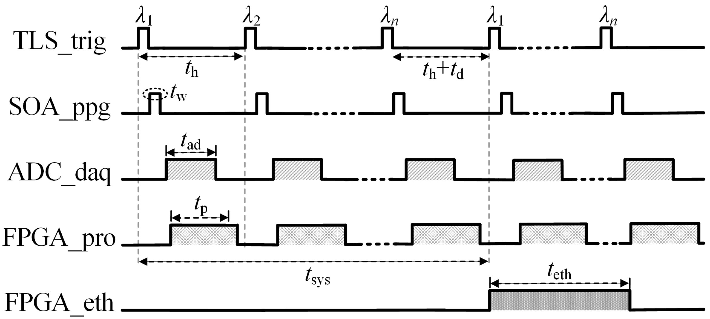
2.1. System Structure

The schematic diagram of the wavelength interrogator is depicted in Figure 1, which contains the optic component part (upper part) and the electronic interrogation part (lower part). In the optic component part, the TLS provides high-speed wavelength adjustments with a wavelength setting time of 5 $\mathsf{\mu }$s, and outputs an electronically generated TTL trigger pulse after each wavelength adjustment. The wavelength scanning range, scanning step, and scanning period are controlled by LabVIEW-based software (LBS). The light from the TLS is modulated into nanosecond pulses by a semiconductor optical amplifier (SOA) driven by a switching circuit (SWC). After being amplified by an Erbium-doped fiber amplifier (EDFA), the pulses are launched into four FBG arrays, of which each array contains thousands of cascade FBG sensors. The reflected signal from each sensing array is converted to an electrical signal by a corresponding photodetector (PD). An isolator is used to prevent the light from feeding back into the light source. The interrogation part realizes real-time processing by interlocking the analog-to-digital converter (ADC) equipped with the FPGA and the LBS. The ADC takes four-channel analog inputs and provides high-speed data transfer to the FPGA. The FPGA, as the central processing unit, synchronizes with the TLS, controls the pulse modulation by the SOA, and acquires the data from the ADC for wavelength interrogation. After interrogation, the wavelength data of all FBGs are transferred to the LBS for further processing, such as filter, display, and record, via the network with a user datagram protocol (UDP).

2.2. Interrogation Frequency

The practical timing of the interrogation is shown in Figure 2. By leading the benefits of parallel processing ability of an FPGA, the interrogation works of four sensing arrays are independently carried out at the same time; hence, we describe the interrogation process of one sensing array in this part for a better understanding.

During each interrogation period $t_{\mathrm{sys}}$, the TLS scans its output wavelength, for example, from ${\lambda }_1$ to ${\lambda }_n$ with a time interval of $t_{\mathrm{h}}$, and then the SOA driven by the FPGA chops the CW light from the TLS into pulses with a pulsewidth of $t_{\mathrm{w}}$. The pulses are injected into the sensing array with a sensing distance of L and grating spacing of $G_{\mathrm{s}}$. Then, the reflected signal from the sensing array is collected for $t_{\mathrm{ad}}$ time and processed within $t_{\mathrm{p}}$ time by the FPGA, using the technique of pipelining. After a delay of $t_{\mathrm{d}}$, the system will start the second interrogation and transfer the first interrogation results to the computer within $t_{\mathrm{eth}}$ time via network.

In response to each laser pulse, successive pulses corresponding to the FBGs return from the sensing array. To distinguish each FBG, the pulsewidth of the laser pulse $t_{\mathrm{w}}$ should satisfy $t_{\mathrm{w}}\le 2G_{\mathrm{s}}{n}_{\mathrm{eff}}/\mathrm{c}$, where $n_{\mathrm{eff}}$ is the effective refractive index of the sensing fiber and $\mathrm{c}$ is the speed of light in a vacuum.

To obtain the sensing information of all the FBGs, the signal-collecting time $t_{\mathrm{ad}}$ should satisfy $t_{\mathrm{ad}}\ge 2L{n}_{\mathrm{eff}}/\mathrm{c}$.

The signal processing will start once the signal is collected. For a high interrogation frequency, the processing time $t_{\mathrm{p}}$ needs to satisfy that $t_{\mathrm{p}}\le t_{\mathrm{h}}$ and $t_{\mathrm{p}}\ge t_{\mathrm{ad}}$.

The time delay $t_{\mathrm{d}}$, with a scale of 1 $\mathsf{\mu }$s, is used to adjust the wavelength from ${\lambda }_n$ to ${\lambda }_1$ and fine-tune the interrogation frequency. The interrogation period $t_{\mathrm{sys}}$ can be expressed as:

$$t_{\mathrm{sys}}=n{t}_{\mathrm{h}}+t_{\mathrm{d}}.$$

(1)

For a real-time interrogation, the transmission time $t_{\mathrm{eth}}$ should be smaller than $t_{\mathrm{sys}}$.

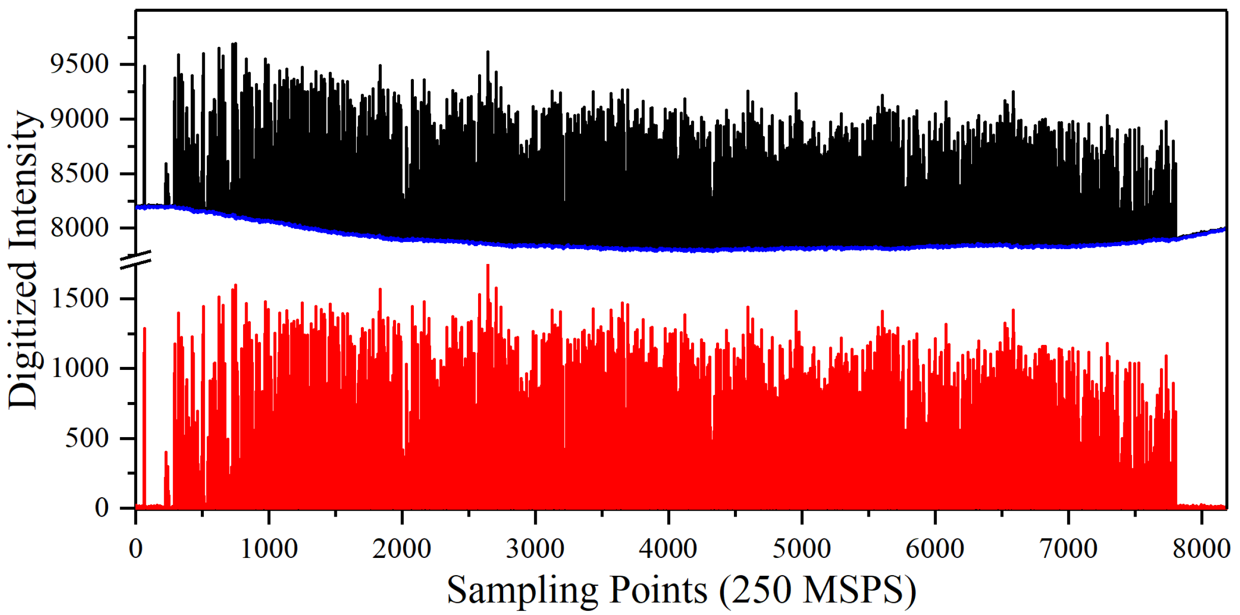
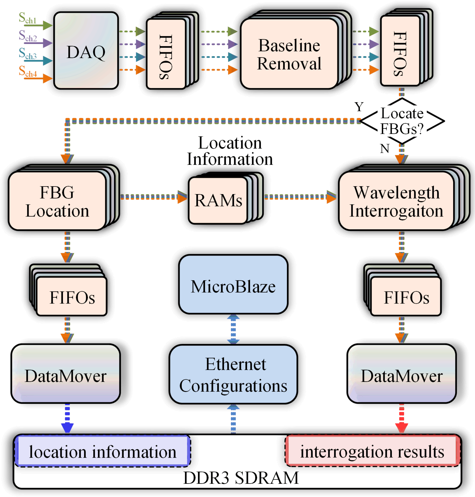
2.3. Signal Processing

Based on the returning pulses train at each wavelength, the reflection spectrum of each FBG can be reconstructed [10]. The reflection spectrum $R_k$ of the kth FBG in the array can be reconstructed based on the returning power $P_{j,k}$ at the jth wavelength:

$$R_k=[P_{1,k},P_{2,k},P_{3,k},\dots ,P_{n,k}].$$

(2)

The Gaussian model is often used to determine the wavelength of the reflection spectrum. However, the Gaussian fitting algorithm does not work well because of non-main lobe sample points [14]. Moreover, the Gaussian fitting algorithm takes over 0.2 s, which is not applicable in real-time systems with many FBGs. This paper adopts the conventional centroid detection algorithm to demodulate the wavelength. The center wavelength ${\lambda }_{\mathrm{c},k}$ of the kth FBG can be calculated by:

$${\lambda }_{\mathrm{c},k}=\frac{{\sum }_{i=1}^n{\lambda }_i{P}_{i,k}}{{\sum }_{i=1}^n{P}_{i,k}}.$$

(3)

We can see that the terms ${\sum }_{i=1}^n{\lambda }_i{P}_{i,k}$ and ${\sum }_{i=1}^n{P}_{i,k}$ are independent and can be calculated at each wavelength. When the wavelength-scanning is ${\lambda }_n$, the center wavelength can be obtained by a division operation.

3. Implementation

As described above, the interrogation period is mainly related to the wavelength-scanning times and the wavelength-scanning interval. In this part, we carefully design an FPGA-based implementation architecture of the interrogator to minimize the time cost of signal processing.

3.1. Signal Conditioning

The FPGA used in this paper is Kintex-7 XC7K325T, equipped on a KC705 evaluation board produced by Xilinx, Inc, owing to the right combination of price and performance. The ADC used in this paper (2 pieces of AD9643, Analog Devices, Inc., Cambridge, MA, USA) takes four-channel 14-bit analog inputs and operates at sampling speeds of up to 250 MSPS. Thus, there will be 8000 sampling points per channel for a 3.2-km sensing array. To avoid cross-clock domains inside the FPGA, we set the system clock equal to 250 MHz. The data sequence $d_{\mathrm{in}}\left(p\right)$ sampled from a sensing channel will be buffered in a high-speed first-in-first-out (FIFO) block.

For some applications where SNR is a crucial parameter, differential transformer coupling is the recommended input configuration while driving the AD9643. However, the signal delivered by the transformer always shows an envelope droop due to its self-inductance-to-resistance ratio [22], as shown by the black line in Figure 3. The baseline drift has to be removed because it changes with different signals, which negatively affects the detection of each FBG. Aiming to solve this problem, and considering the complexity of the algorithm implemented on FPGA, we adopt a polynomial-based baseline-removal algorithm, which is mainly based on simple logic and elementary operations [23]. The simplified algorithm is presented as follows:

1.

Load the parameters of fitting coefficient $f_{\mathrm{coe}}$ from the LBS, and read the first data of the sampled data sequence $d_{\mathrm{in}}\left(1\right)$;

2.

Initialize the baseline sequence $bl\left(1\right)=d_{\mathrm{in}}\left(1\right)$, and output the corrected data $d_{\mathrm{cs}}\left(1\right)=d_{\mathrm{in}}\left(1\right)-bl\left(1\right)=0$;

3.

Continuously read the sampled data sequence $d_{\mathrm{in}}\left(p\right)$, and obtain the baseline sequence $bl\left(q\right)=\min (d_{\mathrm{in}}\left(q\right),bl(q-1)+f_{\mathrm{coe}})$. Then, the corrected data can be calculated by $d_{\mathrm{cs}}\left(q\right)=d_{\mathrm{in}}\left(q\right)-bl\left(q\right)$.

We can see that the above algorithm can be easily implemented on the FPGA in pipeline. For each channel, the function module reads the sampled data sequence from the FIFO, fits the baseline sequence $bl$, and outputs the corrected signal $d_{\mathrm{cs}}$ to a new FIFO block for the next stage of processing. The performance and utilization of the algorithm are estimated by Vivado software. For all the data from four channels, it takes 4 clock cycles to complete one iteration of the loop and 8195 clock cycles to compute 8192 output values with 280 flip-flops (FFs) and 380 look-up tables (LUTs).

It is worth noting that the fitting coefficient $f_{\mathrm{coe}}$ controlled by the LBS is determined by the curvature of the baseline, which varies with different ADC boards. A small $f_{\mathrm{coe}}$ value can help to reduce the effect of baseline, and the variation has to be larger than the noise level. A higher $f_{\mathrm{coe}}$ not only leads to better baseline removal, but also removes some valid and important data, which will be used to reconstruct the spectra of the FBGs. By setting a proper $f_{\mathrm{coe}}$ value, the estimated baseline and the corrected signal are denoted by the blue and red lines in Figure 3, indicating an effective method for removing the baseline drift.

3.2. FBG Location

To achieve real-time FBG signal detection, an advance location process for each FBG is necessary to reduce the time consumed for additional signal processing. Theoretically, each FBG in the array can be identified based on the returning pulses train at the center wavelength of the array. However, affected by the wavelength differences between the FBGs, it is not easy to determine the location of each FBG by utilizing return pulses under one single wavelength in practice. As illustrated in Figure 4, the blue dashed line presents the returning pulses train at the center wavelength (1550.4 nm). We can see that most FBGs reflect the injected light significantly, but some FBGs (such as FBG#5, FBG#6, FBG#10) respond to the 1550.4-nm light slightly. For a better and easier location, light with different wavelengths, such as the black dashed line whose wavelength is close to the center wavelength (1550.6 nm) of FBG#5, FBG#6, and FBG#10, are separately injected into the array. By averaging the reflected signals under different wavelengths, we can see that the processed pulses train is less affected by the wavelength differences, as shown by the red line.

On FPGA side, a counter is used to record the wavelength scanning times, and four dual-port random access memory (RAM) blocks with a depth of $R_{\mathrm{depth}}$, corresponding to four sensing channels, are used to cache the sum of the returning pulses trains. Each returning pulses train has $R_{\mathrm{depth}}$ sampling points. When the counter value $N_{\mathrm{add}}$ lies in the range of (0, $N_s$), the returning pulses trains are summed up; otherwise, the summed result $d_{\mathrm{r}}\left(p\right)$ is used to determine the location of each FBG, where $N_s$ is the total wavelength scanning times. By iterating the data series $d_{\mathrm{r}}\left(p\right)$, those peaks that are greater than the minimum peak height (MPH) are found, corresponding to each FBG. The specific working flow for locating each FBG by utilizing the returning pulses train is described as follows:

1.

Initialize the RAM block and the counter value $N_{\mathrm{add}}$ to zero at power-on. Load the parameters of total wavelength scanning times $N_s$ and minimum peak height $MPH$;

2.

Read the returning pulses train $d_{\mathrm{cs}}\left(p\right)=d_{\mathrm{cs}}\left(1\right),d_{\mathrm{cs}}\left(2\right),\dots ,d_{\mathrm{cs}}\left(R_{\mathrm{depth}}\right)$ from FIFO of the previous stage (baseline removal), load the data stored in the RAM block $d_{\mathrm{r}}\left(p\right)=d_{\mathrm{r}}\left(1\right),d_{\mathrm{r}}\left(2\right),\dots ,d_{\mathrm{r}}\left(R_{\mathrm{depth}}\right)$, and increase $N_{\mathrm{add}}$ by one;

3.

Calculate the sum of $d_{\mathrm{cs}}\left(p\right)$ and $d_{\mathrm{r}}\left(p\right)$, and then store the result back to the RAM;

4.

Repeat steps 2 and 3 until $N_{\mathrm{add}}=N_s$;

5.

Set $N_{\mathrm{add}}$ to zero and construct a RAM block to store the location information $G_{\mathrm{Loc}}\left(s\right)$ of the sensing array. Here, $G_{\mathrm{Loc}}\left(s\right)$ is a data sequence with the local peaks of the $d_{\mathrm{r}}\left(p\right)$, and the parameter $MPH$ is used to avoid the noises. Specially, the first element in $G_{\mathrm{Loc}}\left(s\right)$ stores the number of FBGs.

The location-related functions inside the FPGA are sub-routinized and, thus, can be implemented easily. The summing process (i.e., steps 2 and 3) can be implemented in pipeline, and the data from four channels can be processed in parallel. It takes $R_{\mathrm{depth}}+2$ clock cycles to process $R_{\mathrm{depth}}$ sampling points, in which two extra clock cycles are induced by the iteration latency (number of clock cycles it takes to complete one iteration of the loop). Therefore, it takes about $N_s(R_{\mathrm{depth}}+2)$ clock cycles to obtain the summed result $d_{\mathrm{r}}\left(p\right)$. The peak search function is executed within $R_{\mathrm{depth}}$ clock cycles, and $R_{\mathrm{depth}}$ more clock cycles are consumed to output the location information $G_{\mathrm{Loc}}\left(s\right)$ to the following processing stage. As a result, it would take $N_s(R_{\mathrm{depth}}+2)+2R_{\mathrm{depth}}$ clock cycles to determine the location of each FBG. When $R_{\mathrm{depth}}$ = 8192, the resource utilization is about 1018 FFs, 1191 LUTs, and 44 RAM blocks for four channels.

Because the location information of the sensing array hardly changes once the sensing array is connected to the system, the location process can be executed only once. Thus, the time consummation of this part can be neglected, and we can apply a larger $N_s$ for a clear line of the returning pulses train.

3.3. Wavelength Interrogation

Conventional wavelength-interrogation systems usually reconstruct the spectra of all the FBGs, which means we should complete the wavelength scanning and then obtain the wavelength information by analyzing the spectrum of each FBG [24]. However, as the number of FBGs increases, a large number of spectra data points require more storage or buffer resources, and the dataflow between functions is detrimental to real-time interrogation. From Equation (3), we can learn that the centroid-calculation algorithm can individually process each spectra data point during the wavelength scanning, thereby avoiding the storage and transmission of a large number of data points. To further accelerate the calculation, especially the multiplication operation, a built-in DSP48E block is used for one channel, and the wavelength parameter ${\lambda }_i$ is replaced by i, where $i=1,2,\dots ,n$. Additionally, this work operates with fixed-point arithmetic, the bit width of the input data and the product is respectively adjusted to 14 bit and 32 bit, and the total wavelength scanning times n in each period is fixed.

For each channel during the interrogation, the location information $G_{\mathrm{Loc}}\left(s\right)$ is stored in a RAM block; two other RAM blocks $Num$ and $Den$ with a depth of $G_{\max }$ are constructed to, respectively, store the numerator and denominator results of Equation 3 for each FBG, where $G_{\max }$ is the maximum number of FBGs. The returning pulses trains at different wavelengths are read from the FIFO of the previous stage (baseline removal), while the lasing wavelength scanns from ${\lambda }_1$ to ${\lambda }_n$. At each wavelength, the peak value $P_{\max }$ of each pulse corresponding to the reflectivity of each FBG is obtained by querying the location data stored in $G_{\mathrm{Loc}}\left(s\right)$. Meanwhile, the numerator and denominator results of each FBG are, respectively, calculated and stored in $Num$ and $Den$ blocks. A counter is used to record the wavelength scanning times. After each scanning period (i.e., the count value $N_{\mathrm{intg}}$ equal to n), the wavelengths of the FBGs are calculated by a division operation and then outputted to a FIFO block for data delivery. The specific interrogation process is shown as follows:

1.

Before the interrogation, initialize the counter value $N_{\mathrm{intg}}$ to zero, reset two RAM blocks $Num$ and $Den$ to zero, and load parameter n;

2.

Read the returning pulses train $d_{\mathrm{cs}}\left(p\right)=d_{\mathrm{cs}}\left(1\right),d_{\mathrm{cs}}\left(2\right),\dots ,d_{\mathrm{cs}}\left(R_{\mathrm{depth}}\right)$ from previous FIFO, load the location information $G_{\mathrm{Loc}}\left(s\right)$, and increase $N_{\mathrm{intg}}$ by one;

3.

Obtain the number of FBGs $G_{\mathrm{Loc}}\left(1\right)$, and then calculate the numerator and denominator terms for each FBG by:

• Seeking the peak value $P_{\max }$ of jth FBG around $d_{\mathrm{cs}}\left(G_{\mathrm{Loc}(\mathrm{j}+1)}\right)$;
• $Num\left(j\right)=Num\left(j\right)+P_{\max }*N_{\mathrm{intg}}$, and $Den\left(j\right)=Den\left(j\right)+P_{\max }$;

4.

Repeat steps 2 and 3 until $N_{\mathrm{intg}}=n$;

5.

Set $N_{\mathrm{intg}}$ to zero, calculate the wavelength result of each FBG, and then reset $Num$ and $Den$ to zero;

6.

Repeat steps 2, 3, 4, and 5 for a continuous-running interrogation.

It takes $R_{\mathrm{depth}}$ clock cycles to read $d_{\mathrm{cs}}\left(p\right)$ of all channels due to the parallel processing ability of an FPGA. The time consumption on Step 3 is crucial to real-time interrogation. To obtain accurate peak values, three sampling points are accessed and processed for each FBG. Moreover, extra clock cycles are needed for the multiplication operation and the access to $G_{\mathrm{Loc}}\left(s\right)$, $Num$, and $Den$. As a result, the iteration latency is estimated to be 11 by the Vivado tool, which means 11 clock cycles are needed to process one FBG. When the loop is pipelined, the loop initiation interval (number of clock cycles before the next iteration of the loop starts to process data) is estimated to be 2; thus, the latency of this part is $2*G_{\mathrm{Loc}}\left(1\right)+9$ clock cycles. In the fifth step, the wavelength results of four channels are successively outputted to a FIFO block for data delivery; the iteration latency affected mainly by the divider is estimated to be 39, and the loop initiation interval is 1 when the loop is pipelined. Thus, the latency of this step is $4*(G_{\mathrm{Loc}}\left(1\right)+38)$ clock cycles. Furthermore, the results (16-bit) from two channels are combined to transfer, so the latency becomes $2*(G_{\mathrm{Loc}}\left(1\right)+38)$ clock cycles.

Assuming that $R_{\mathrm{depth}}=8192$ and $G_{\max }=1024$, the resource utilization is about 9828 FFs, 7043 LUTs, 4 DSP48Es, and 44 BRAMs. It is worth noting that four dividers consume lots of logic resources (8460 FFs, and 6268 LUTS). For FPGAs with less logic resources, we can transfer both the numerator and denominator terms to the computer and perform a division operation on the computer side. In that case, the data-transfer time will double.

3.4. Data Transfer

Figure 5 shows the system design for signal processing. As described before, the signal acquired by DAQ is firstly performed to remove the baseline drift. Then, the signal will flow to either the FBG location part or the wavelength interrogation part, which depends on the control of LBS. When a new sensing array is connected to the system, the first thing to do is to locate the FBGs. The location information will be stored in RAM for wavelength interrogation. The location information will also be transferred to an external double data-rate three-synchronous dynamic random access memory (DDR3 SDRAM) by an advanced extensible interface 4 (AXI4)-based data mover, whose transfer rate is up to several Gbps. In addition, The interrogation results will be transferred to the DDR3 SDRAM by the other data mover. Some FIFOs are used to buffer the processed data.

To achieve a real-time wavelength interrogation, a high-throughput data transferring solution is required. This demand is resolved using an open-source lightweight IP (lwIP) networking stack, which can accept data transfers at rates of up to several-hundred Mbps. The lwIP software is customized to run on a MicroBlaze-based Xilinx embedded system, which can co-operate with programmable hardware, improving the flexibility of the interrogation system.

During the interrogation, the results of four channels of a single measurement will take 16-bits per FBG * $G_{\max }$ per channel * four channels. Ignoring the time consumption on signal processing, the minimum interrogation period $t_{\mathrm{sys}}$ would be $n{t}_{\mathrm{ad}}$ according to Equation (1). Further, the required transfer rate can be calculated. Assuming that four pieces of 3.2-km sensing fibers, each containing 1024 FBGs, are connected to the system, and that the wavelength is scanned with a 3-nm dynamic range and 20-pm interval, the storage usage is about 8 kB, and the interrogation period is about 4.8 ms. Therefore, the required maximum transfer rate is about 13 Mbps, which can be easily realized using lwIP software. At the transport layer, we adopt UDP, which is more efficient in terms of latency and bandwidth, to communicate with LBS.

On the computer side, the transferred data are received and processed by the LBS, as shown in Figure 6. The summed returning pulses train of each channel is displayed in the right part of Figure 6a. The traces of the first and the fourth channels show the overall view of corresponding returning pulses trains. The traces of the second and the third channels, respectively, show the front-end and tail-end of corresponding returning pulses trains. We can see that the intensity of the returning pulses train decreases with the sensing distance, and the intensity of adjacent pulses fluctuates slightly, which is beneficial to the locating of each FBG. In the left part, we can adjust the scanning parameters of the TLS and the fitting coefficient for the baseline removal. Additionally, the location information (such as sensing length and sensing numbers) of each channel is shown in the left part. During the interrogation, the wavelength information of one channel and three FBGs of each channel can be displayed in real time, as shown in Figure 6b. We can also post-process the real-time wavelength data in this panel, such as storage and filter.

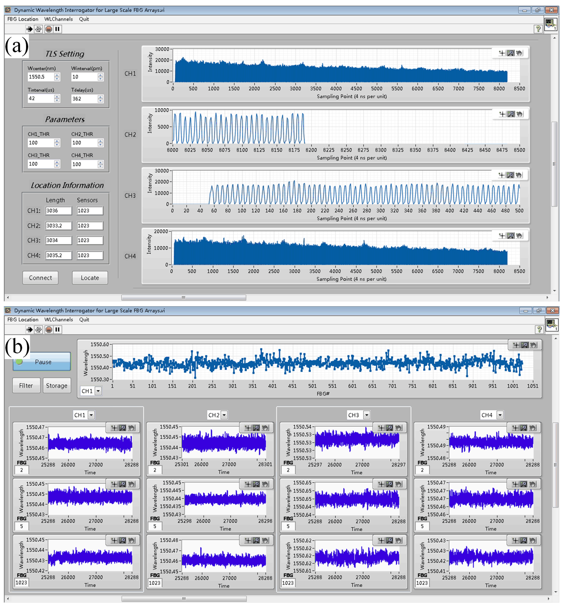
4. Experiment

4.1. Sensing Performance

To evaluate the performance of the proposed interrogation system, four 3.4-km sensing arrays with a spatial resolution of 3 m, a center wavelength of 1550.5 nm, and a reflectivity of about $-45$ dB are connected to the system. The $G_{\max }$ of each channel is 1024 so that all channels are operating under full load. The FBG location process is completed within 1.5 s. Then, the interrogation period and precision are tested and analyzed as follows.

According to the analysis in Section 2, the time-consumption distribution of the interrogation is calculated, as illustrated in Figure 7. The TTL trigger pulse from TLS has a pulse width of 1 $\mathsf{\mu }$s. Within a slight time-delay $t_{\mathrm{int}}$ after detecting the rising edge of the trigger pulse, the FPGA controls the pulse modulation of SOA and launches the acquisition of DAQ. Considering the limitation of $G_{\max }$, the sampling length $R_{\mathrm{depth}}$ at each wavelength is set to 8192. Therefore, the signal-collecting time $t_{\mathrm{ad}}$ is about 32.77 $\mathsf{\mu }$s, and the signal-conditioning part takes 32.78 $\mathsf{\mu }$s. It is worth noting that only 1∼2 clock cycles are required to deliver data from one part to the other because the FPGA operates in pipeline, as shown by the blue circle. For previous $n-1$ wavelengths, the interrogation part takes 32.77 $\mathsf{\mu }$s to read the sampling data, and then takes 8.23 $\mathsf{\mu }$s to perform the calculation. At the last wavelength ${\lambda }_n$, an extra 8.5 $\mathsf{\mu }$s are required to obtain the wavelength information and output the data to the next part. Due to the high performance of AXI4 and LwIP, the time consumption on these parts is negligible. Consequently, the scanning interval $t_{\mathrm{h}}$ is approximately 42 $\mathsf{\mu }$s, and the interrogation period $t_{\mathrm{sys}}$ is $(42n+t_{\mathrm{d}})$$\mathsf{\mu }$s, where $t_{\mathrm{d}}\ge 8.5$$\mathsf{\mu }$s. We can see that a small n value indicates a short response time. However, the dynamic range or spectral resolution is negatively affected by a small n value.

Taking $n=150$ as an example, the interrogation period is 150 Hz when $t_{\mathrm{d}}=367$$\mathsf{\mu }$s. Here, the frequency accuracy can be ensured by fine-tuning the $t_{\mathrm{d}}$ value. The scanning range $R_{\mathrm{scan}}$ changes with the scanning interval ($I_{\mathrm{scan}}$) through the relation $R_{\mathrm{scan}}=n{I}_{\mathrm{scan}}$. When $I_{\mathrm{scan}}=10$ pm, the scanning range is 1.5 nm (from 1550 nm to 1551.49 nm), and the interrogation error within 10 s is shown in Figure 8a. We can see that the wavelengths slightly vary from $\pm 1.0$ pm to $\pm 2.7$ pm, with a mean value of $\pm 1.6$ pm. When $I_{\mathrm{scan}}=20$ pm, the scanning range is widened to 3 nm, and the average value of standard deviation (STD) is $\pm 5.9$ pm. Continuing to increase $I_{\mathrm{scan}}$, we can obtain a more extensive scanning range, but the interrogation error also increases. When $I_{\mathrm{scan}}=40$ pm, the scanning range is 6 nm, and the maximum wavelength fluctuation is 47.4 pm, as shown in Figure 8d. The reason behind the large interrogation error is that the bandwidth of our FBGs is less than 100 pm [25]. Consequently, the best way to increase the scanning range is to increase the n value, which undoubtedly reduces the interrogation frequency.

Furthermore, sinusoidal waves of 1 Hz, 5 Hz, and 10 Hz with amplitudes of 30 voltage (equivalent 2.67 $\mathsf{\mu }$m peak-to-peak length change) are generated separately by the function generator to oscillate a stacked piezoelectric transducer (PZT), applying a 267 $\mathsf{\mu }\epsilon$ peak-to-peak dynamic strain variation on one FBG (grating length = 10 mm). The wavelength trace of the FBG and its fast Fourier transform (FFT) results are displayed in Figure 9. The spectra show that the transformed frequency corresponds to the given frequency, and the maximum frequency error is 0.7% at 1 Hz, verifying the interrogation frequency. Moreover, the peak-to-peak wavelength shift in Figure 9a is about 267 pm, which is similar to the strain characteristic of the ordinary grating.

4.2. Distributed Real-Time Sensing

Finally, we evaluated the multi-channel and real-time measurement of reflection wavelength using instantaneous vibrations. The first FBG of each channel is attached to the PZT, and vibrations are applied. The vibration frequency of the PZT is set to 5 Hz, and the vibration is applied every 300 s. Figure 10a shows the interrogation results. The wavelength of each FBG fluctuates greatly every 300 s when vibrations are applied. Figure 10b,c show the zoomed-in view of the wavelength trace when the first and third vibration signals are applied, respectively. The wavelength of each FBG can be measured as a sinusoidal vibration with a vibration frequency of 5 Hz, and the vibrations change with the same phase, indicating a stable real-time measurement without data loss.

5. Conclusions

In conclusion, we presented a complete design of a simple and practical FPGA-based wavelength-interrogation system for thousands of identical FBGs. The signal-processing system implements an FPGA for performing real-time high-speed sampling, processing, and transfers. The design contains the functional modules with carefully optimized pipeline architecture: the signal-conditioning module, the FBG location module, the wavelength-interrogation module, and the LBS module. A sensing frequency of 150 Hz with 3-nm dynamic range and $\pm 5.9$-pm precision is achieved over four 3-km sensing arrays, each containing over 1000 FBGs. The programming for parallel processing can easily cope with the expansion of the sensing channel. One way to speed up the interrogation process further is to reduce the spectral resolution, which often produces poor results. The following work will emphasize the implementation of a feasible algorithm for low spectral resolution.

References

- Zhang, X.; Liang, D.; Zeng, J.; Asundi, A. Genetic algorithm-support vector regression for high reliability SHM system based on FBG sensor network. Opt. Lasers Eng. 2012, 50, 148–153. [Google Scholar] [CrossRef]
- Mieloszyk, M.; Majewska, K.; Zywica, G.; Kaczmarczyk, T.Z.; Jurek, M.; Ostachowicz, W. Fibre Bragg grating sensors as a measurement tool for an organic Rankine cycle micro-turbogenerator. Measurement 2020, 157, 107666. [Google Scholar] [CrossRef]
- Talebinejad, I.; Fischer, C.; Ansari, F. Serially multiplexed FBG accelerometer for structural health monitoring of bridges. Smart. Struct. Syst. 2009, 5, 345–355. [Google Scholar] [CrossRef]
- Liu, Q.; Wang, F.; Li, J.; Xiao, W. A hybrid support vector regression with multi-domain features for low-velocity impact localization on composite plate structure. Mech. Syst. Signal Process. 2021, 154, 107547. [Google Scholar] [CrossRef]
- Xia, L.; Wu, Y.; Rahubadde, U.; Li, W. TDM Interrogation of Identical Weak FBGs Network Based on Delayed Laser Pulses Differential Detection. IEEE Photonics J. 2018, 10, 1–8. [Google Scholar] [CrossRef]
- Ou, Y.; Zhou, C.; Qian, L.; Fan, D.; Cheng, C.; Guo, H.; Xiong, Z. Large WDM FBG Sensor Network Based on Frequency-Shifted Interferometry. IEEE Photonics Technol. Lett. 2017, 29, 535–538. [Google Scholar] [CrossRef]
- Hwang, D.; Seo, D.C.; Kwon, I.B.; Chung, Y. Restoration of Reflection Spectra in a Serial FBG Sensor Array of a WDM/TDM Measurement System. Sensors 2012, 12, 12836–12843. [Google Scholar] [CrossRef] [Green Version]
- Liu, Q.; Li, J.; Wu, L.; Wang, F.; Xiao, W. A novel bat algorithm with double mutation operators and its application to low-velocity impact localization problem. Eng. Appl. Artif. Intell. 2020, 90, 103505. [Google Scholar] [CrossRef]
- Zhang, X.; Liu, X.; Zhang, F.; Sun, Z.; Min, L.; Li, S.; Jiang, S.; Li, M.; Wang, C.; Ni, J. Reliable high sensitivity FBG geophone for low frequency seismic acquisition. Measurement 2018, 129, 62–67. [Google Scholar] [CrossRef]
- Wang, Y.; Gong, J.; Dong, B.; Wang, D.Y.; Shillig, T.J.; Wang, A. A Large Serial Time-Division Multiplexed Fiber Bragg Grating Sensor Network. J. Lightw. Technol. 2012, 30, 2751–2756. [Google Scholar] [CrossRef]
- Chan, C.C.; Jin, W.; Ho, H.; Suleyman Demokan, M. Performance analysis of a time-division-multiplexed fiber Bragg grating sensor array by use of a tunable laser source. IEEE J. Sel. Top. Quantum Electron. 2000, 6, 741–749. [Google Scholar] [CrossRef]
- Dai, Y.; Li, P.; Liu, Y.; Asundi, A.; Leng, J. Integrated real-time monitoring system for strain/temperature distribution based on simultaneous wavelength and time division multiplexing technique. Opt. Lasers Eng. 2014, 59, 19–24. [Google Scholar] [CrossRef]
- Luo, Z.; Wen, H.; Guo, H.; Yang, M. A time- and wavelength-division multiplexing sensor network with ultra-weak fiber Bragg gratings. Opt. Express 2013, 21, 22799–22807. [Google Scholar] [CrossRef] [PubMed] [Green Version]
- Hu, C.; Bai, W. High-Speed Interrogation for Large-Scale Fiber Bragg Grating Sensing. Sensors 2018, 18, 665. [Google Scholar] [CrossRef] [PubMed] [Green Version]
- Wang, Y.; Gong, J.; Wang, D.Y.; Dong, B.; Bi, W.; Wang, A. A Quasi-Distributed Sensing Network with Time-Division-Multiplexed Fiber Bragg Gratings. IEEE Photon. Technol. Lett. 2011, 23, 70–72. [Google Scholar] [CrossRef]
- Ball, G.A.; Morey, W.W.; Cheo, P.K. Fiber laser source/analyzer for Bragg grating sensor array interrogation. J. Lightw. Technol. 1994, 12. [Google Scholar] [CrossRef]
- Huber, R.; Adler, D.C.; Fujimoto, J.G. Buffered Fourier domain mode locking: Unidirectional swept laser sources for optical coherence tomography imaging at 370,000 lines/s. Opt. Lett. 2006, 31, 2975–2977. [Google Scholar] [CrossRef]
- Askins, C.G.; Putnam, M.A.; Friebele, E.J. Instrumentation for interrogating many-element fiber Bragg grating arrays. In Proceedings of the Smart Structures and Materials 1995: Smart Sensing, Processing, and Instrumentation, San Diego, CA, USA, 26 February–3 March 1995; Volume 2444, pp. 257–266. [Google Scholar] [CrossRef]
- Yang, Y.; Wu, J.; Wang, M.; Wang, Q.; Yu, Q.; Chen, K.P. Fast Demodulation of Fiber Bragg Grating Wavelength from Low-Resolution Spectral Measurements Using Buneman Frequency Estimation. J. Lightw. Technol. 2020, 38, 5142–5148. [Google Scholar] [CrossRef]
- Monmasson, E.; Cirstea, M.N. FPGA Design Methodology for Industrial Control Systems—A Review. IEEE Trans. Ind. Electron. 2007, 54, 1824–1842. [Google Scholar] [CrossRef]
- Cui, K.; Peng, W.; Ren, Z.; Qian, J.; Zhu, R. FPGA-based interrogation controller with optimized pipeline architecture for very large-scale fiber-optic interferometric sensor arrays. Opt. Lasers Eng. 2019, 121, 389–396. [Google Scholar] [CrossRef]
- Huang, S.M.; Stott, A.L.; Green, R.G.; Beck, M.S. Electronic transducers for industrial measurement of low value capacitances. J. Phys. E Sci. Instrum. 1988, 21, 242–250. [Google Scholar] [CrossRef]
- Leger, M.N.; Ryder, A.G. Comparison of Derivative Preprocessing and Automated Polynomial Baseline Correction Method for Classification and Quantification of Narcotics in Solid Mixtures. Appl. Spectrosc. 2006, 60, 182–193. [Google Scholar] [CrossRef] [PubMed]
- Werzinger, S.; Bergdolt, S.; Engelbrecht, R.; Thiel, T.; Schmauss, B. Quasi-Distributed Fiber Bragg Grating Sensing Using Stepped Incoherent Optical Frequency Domain Reflectometry. J. Lightwave Technol. 2016, 34, 5270–5277. [Google Scholar] [CrossRef]
- Guo, H.; Tang, J.; Li, X.; Zheng, Y.; Yu, H.; Yu, H. On-line writing identical and weak fiber Bragg grating arrays. Chin. Opt. Lett. 2013, 11, 030602. [Google Scholar]
Publisher’s Note: MDPI stays neutral with regard to jurisdictional claims in published maps and institutional affiliations. |
© 2022 by the authors. Licensee MDPI, Basel, Switzerland. This article is an open access article distributed under the terms and conditions of the Creative Commons Attribution (CC BY) license (https://creativecommons.org/licenses/by/4.0/).
Share and Cite
Wang, J.; Fu, X.; Gao, H.; Gui, X.; Wang, H.; Li, Z. FPGA-Based Dynamic Wavelength Interrogation System for Thousands of Identical FBG Sensors. Photonics 2022, 9, 79. https://doi.org/10.3390/photonics9020079
Wang J, Fu X, Gao H, Gui X, Wang H, Li Z. FPGA-Based Dynamic Wavelength Interrogation System for Thousands of Identical FBG Sensors. Photonics. 2022; 9(2):79. https://doi.org/10.3390/photonics9020079
Chicago/Turabian StyleWang, Jiaqi, Xuelei Fu, Hui Gao, Xin Gui, Honghai Wang, and Zhengying Li. 2022. "FPGA-Based Dynamic Wavelength Interrogation System for Thousands of Identical FBG Sensors" Photonics 9, no. 2: 79. https://doi.org/10.3390/photonics9020079
APA StyleWang, J., Fu, X., Gao, H., Gui, X., Wang, H., & Li, Z. (2022). FPGA-Based Dynamic Wavelength Interrogation System for Thousands of Identical FBG Sensors. Photonics, 9(2), 79. https://doi.org/10.3390/photonics9020079