Compressive Bidirectional Reflection Distribution Function-Based Feature Extraction Method for Camouflaged Object Segmentation

Abstract

Camouflaged target segmentation has been widely used in both civil and military applications, such as wildlife behaviour monitoring, crop pest control, and battle reconnaissance. However, it is difficult to distinguish camouflaged objects and natural backgrounds using traditional grey-level feature extraction. In this paper, a compressive bidirectional reflection distribution function-based feature extraction method is proposed for effective camouflaged object segmentation. First, multidimensional grey-level features are extracted from multiple images with different illumination angles in the same scene. Then, the multidimensional grey-level features are expanded based on Chebyshev polynomials. Next, the first several coefficients are integrated as a new optical feature, which is named the compressive bidirectional reflection distribution function feature. Finally, the camouflaged object can be effectively segmented from the background by compressive feature clustering. Both qualitative and quantitative experimental results prove that our method has remarkable advantages over conventional single-angle or multi-angle grey-level feature-based methods in terms of segmentation precision and running speed.

1. Introduction

Camouflaged object segmentation has been extensively applied in many fields, e.g., crop pest control [1,2,3,4], disaster rescue [5,6], and battlefield scout [7,8,9]. Conventional segmentation methods usually use one-dimensional or multidimensional grey-level features to distinguish the object of interest from a natural background. However, there are some technological difficulties in these algorithms. On the one hand, the segmentation precision is hard to guarantee, since the grey values of camouflaged object and background are close to each other and the boundary line is blurred. Furthermore, the multidimensional grey-level feature-based methods always suffer from a large amount of computation and serious data redundancy, which makes it difficult to improve the computing speed of the segmentation algorithm. Therefore, it is of great necessity to further design new camouflaged object segmentation methods by means of exploiting other effective optical features.

Recent research progress has shown that there are two main types of camouflaged object segmentation methods based on grey-level features, including one-dimensional grey-level feature-based approaches and multidimensional grey-level feature-based approaches. Some methods use the one-dimensional grey-level feature for object segmentation. To solve the segmentation difficulties caused by brightness and contrast changes, varying inclination and shadow, Goccia et al. [10] optimised the feature weights and the prototype sets by a new gradient-based learning algorithm to achieve good recognition performances. To discriminate the individual objects in natural outdoor scenes, Zhao et al. [11] converted the obtained RGB image into an HSI image, and used the H grey-level threshold to segment out the object region in the image. For separating the camouflaged objects from the image with noise and shadow, Zheng et al. [12] introduced a mean-shift procedure into the segmentation algorithm based on multiple colour features. To overcome the difficulty of object detection caused by nonobvious shadow, Chen et al. [13] proposed a detection method based on the image grey value feature, which avoided the dependence of image on solar elevation. In order to achieve accurate segmentation of objects in a natural environment, Guo et al. [14] proposed an image segmentation method combining the crow search algorithm and K-means clustering algorithm, by which the segmentation accuracy of the proposed algorithm was significantly improved. However, these algorithms were conducted based on the considerable difference between object and background. When the grey values of object and background are close to each other, the accuracy of the algorithms will be reduced. Some other methods use multidimensional grey-level features extracted from a series of images to segment the object from background. To explore methods for rapid detection of different leaf objects, Liu [15] extracted feature bands from images with multiple light angles and multispectral bands to find the most suitable angle and band for distinguishing healthy leaves from diseased ones. To analyse the difference between the camouflaged object and different backgrounds in hyperspectral images, Yan et al. [16] evaluated the camouflage effect of a camouflaged object in the background from spectral reflectance, information theory, spectral angle, and spectral gradient, respectively. For avoiding the problem that some objects can only be detected at specific angles, Yang [17] proposed a method of object detection using multiple images taken under a multi-angle light source. To improve the accuracy of textile colour segmentation, Wu [18] proposed a method based on hyperspectral imaging to obtain the colour number of textiles by clustering the multidimensional features. Wang et al. [19] selected several distinct characteristic bands, based on which they set a threshold of the image to segment the objects from the similar background. Wang et al. [20] acquired many images of an object under different lighting conditions to obtain samples of the surface’s BRDF, which help to separate the material types by segmentation. Skaff [21] classified materials using illumination by spectral light from multiple different incident angles, where the incident angle and/or spectral content of each light source was selected based on a mathematical clustering analysis of training data. However, their algorithms required a lot of image collection work and a large amount of calculation to achieve the appropriate feature dimensions, which led to a low speed of computing.

In conclusion, the existing methods are deficient in accuracy and speed, mainly because (1) the one-dimensional grey-level feature of the camouflaged object is very close to background; (2) when the camouflaged object and background are segmented by multidimensional grey-level feature-based methods, there is serious data redundancy, which leads to excessive computation. To solve these problems, a compressive bidirectional reflection distribution function (BRDF)-based feature extraction method is proposed. First, the grey-level feature is extracted from a single frame image. The one-dimensional grey levels extracted from multiple images with different illumination angles constitute the multidimensional grey-level feature. Then, we expand the multidimensional grey-level features by Chebyshev polynomials. Next, the first several coefficients of the polynomials are used as the compressive BRDF feature. Finally, we segment the camouflaged object from background by clustering the compressive BRDF feature of each pixel. The method can be used for the detection of small camouflaged objects by near-earth UAVs and the detection of large ground camouflaged objects by geostationary satellites.

The main contributions of our study can be summarised as follows:

• A multidimensional feature extraction method using multi-angle illumination images is proposed to improve the accuracy of object segmentation. The influence of the illumination image on reflectance is considered to help enrich the details of object;
• We present a compression method for multidimensional BRDF features to improve the computing speed of feature clustering. In addition, the degree of retention of valid information during the compression process is also considered;
• Experimental results demonstrate the usefulness and effectiveness of the proposed compressive BRDF feature extraction method in both segmentation accuracy and execution time.

This paper is organised as follows: Section 2 introduces the background of our study; in Section 3, the camouflaged object segmentation method based on compressive BRDF feature extraction is introduced in detail; Section 4 discusses both the quantitative and qualitative experimental results; finally, a summary of this work is drawn in Section 5.

2. Background

By reviewing the conventional object segmentation methods based on multiple features, it can be found that these methods are based on the difference between the object and background in some physical properties. We focus on the differences in reflectance and roughness between the object and background [22]. In this section, the BRDF model is introduced. BRDF describes the relative amount of reflected radiation of incident irradiation, expressed as [23]

$$f\left({\theta }_i,{\phi }_i,{\theta }_r,{\phi }_r,\lambda \right)=\frac{d{L}_r\left({\theta }_r,{\phi }_r,\lambda \right)}{d{E}_i\left({\theta }_i,{\phi }_i,\lambda \right)}$$

(1)

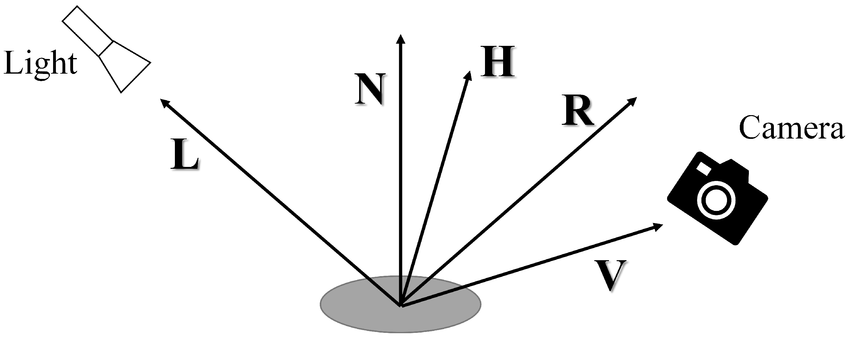
where ${\theta }_i$ is the incident zenith angle, ${\theta }_r$ is the emergent zenith angle, ${\phi }_i$ is the incident orientation angle, ${\phi }_r$ is the emergent orientation angle, and $\lambda$ means the wavelength of incident light. In Equation (1), $d{L}_r\left(\mathrm{W}{·\mathrm{m}}^{-2}·{\mathrm{sr}}^{-1}·{\mathsf{\mu }\mathrm{m}}^{-1}\right)$ represents the radiance in the emergent direction and $d{E}_i\left(\mathrm{W}{·\mathrm{m}}^{-2}·{\mathsf{\mu }\mathrm{m}}^{-1}\right)$ represents the irradiance in the incident direction. Figure 1 shows the light angles in BRDF model.

Researchers have proposed many BRDF models to describe different scenes. One of the classical models is the Cook-Torrance model [24], which assumes that the surface of the medium is composed of a series of plane elements whose direction vectors satisfy Gaussian distribution. The Cook-Torrance model can be expressed as

$$F\left({\theta }_i,{\phi }_i,{\theta }_r,{\phi }_r,\lambda \right)=\frac{D·G}{4cos{\theta }_{i}cos{\theta }_r}$$

(2)

where D denotes the facet slope distribution function and G represents the geometrical attenuation factor. The values of D and G are connected with the changes in incident angle and emergent angle of light.

The surfaces of the object and background are observed as a mass of tiny elements. Figure 2 shows the reflection process occurring on the element of surface.

As shown in Figure 2, L is the unit vector in the direction of light source. N is the unit surface normal. H is the unit internal bisector of V and L. R is the unit vector in the reflection direction of incident light. V is the unit vector in the direction of the viewer. The surface element is not an ideal smooth surface. The facet slope distribution function D is expressed as

$$D=\frac{exp\left(-{\left(\frac{tan\alpha }{\sigma }\right)}^2\right)}{\pi {\sigma }^2{\cos }^4\alpha }$$

(3)

$$tan\alpha =\frac{1-{\left(\mathbf{H}·\mathbf{N}\right)}^2}{{\left(\mathbf{H}·\mathbf{N}\right)}^2}$$

(4)

where $\alpha$ is the angle between N and H, and $\sigma$ is the root mean square slope of facets. The value of D is related to the roughness of the material surface.

The geometrical attenuation factor G is expressed as

$$G=min\left(1,\frac{2\left(\mathbf{N}·\mathbf{H}\right)\left(\mathbf{N}·\mathbf{V}\right)}{\mathbf{H}·\mathbf{V}},\frac{2\left(\mathbf{N}·\mathbf{H}\right)\left(\mathbf{N}·\mathbf{L}\right)}{\mathbf{H}·\mathbf{L}}\right)$$

(5)

In other words, G means the degree to which the small element is obscured from incident light; so, it is related to the reflectivity of the material surface.

In this paper, we conduct object segmentation on a scene in which both the camouflaged object and background exist. The Cook-Torrance model is applicable, as it considers both specular and diffuse reflectance components. Equation (2) has several input parameters. We examined the relationship between the reflectance and one of the input parameters, to make the feature of material easy to observe. The following assumptions are given:

$${\phi }_i-{\phi }_r={180}^{\circ }$$

(6)

$$\lambda =C$$

(7)

$${\theta }_r={45}^{\circ }$$

(8)

$${\theta }_i\in [-{90}^{\circ },{90}^{\circ }]$$

(9)

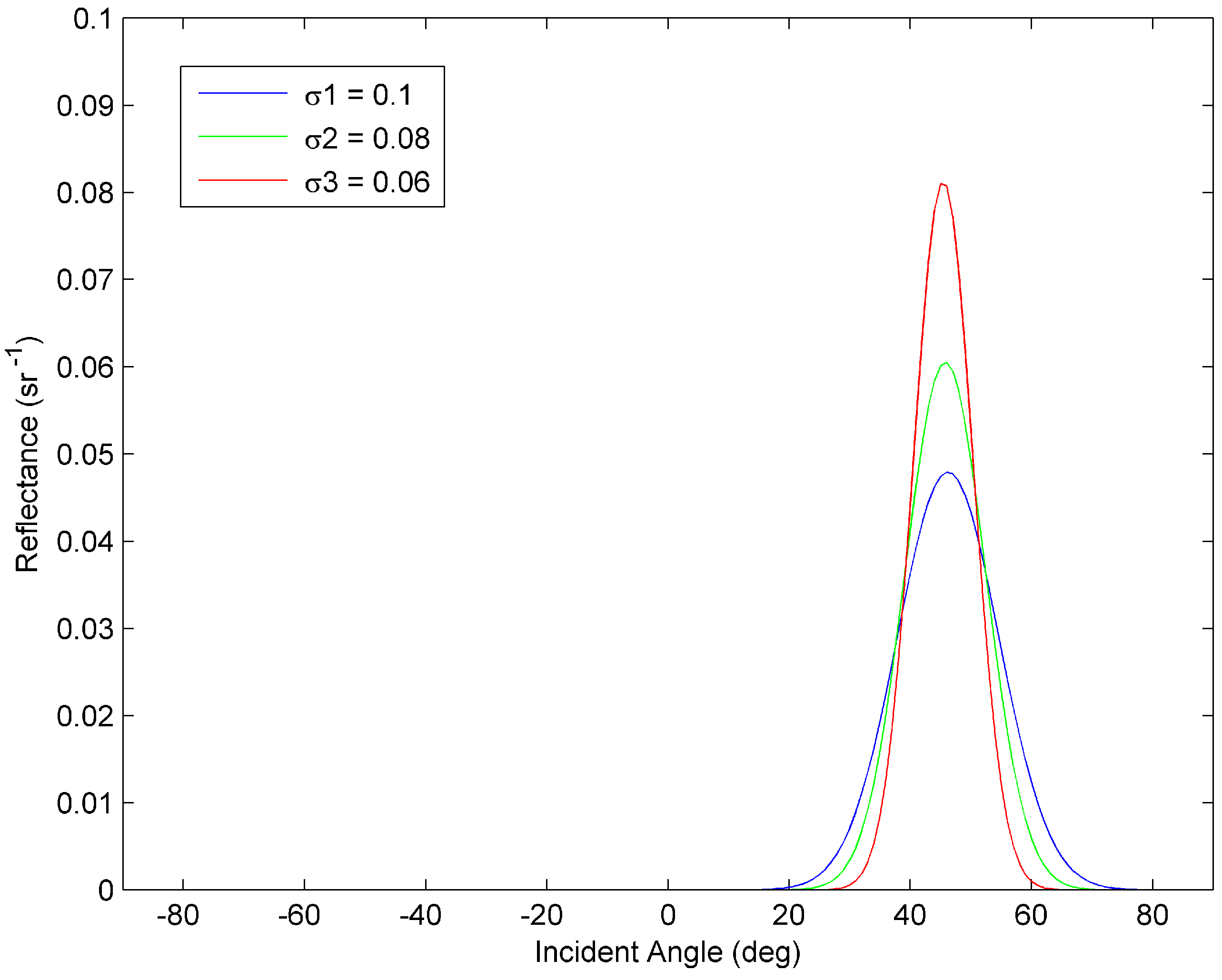
where C stands for a constant in the visible wavelength range. Equation (3) means the incident and emergent angles are in the same plane. Then, Equation (2) can be expressed as a function with ${\theta }_i$ as the only independent variable. Figure 3 shows the Cook-Torrance model with the above assumptions.

As shown in Figure 3, the curves of reflectance and incident angle are related to $\sigma$, which represents the root mean square slope of facets and has an effect on the value of D. The camouflaged object has a different material from the background. Their BRDF curves are usually not consistent. Therefore, the object segmentation method can be implemented based on the BRDF feature.

3. Model Construction of Camouflaged Object Segmentation Method Based on Compressive BRDF Feature Extraction

In order to improve the accuracy and speed of the camouflaged object segmentation method, a compressive BRDF feature extraction method is introduced in this section. The compressive BRDF feature is used in image clustering to achieve the segmentation of the camouflaged object. The compressive BRDF feature is achieved by reducing the dimension of multidimensional grey-level features extracted from the multi-illumination angle images. It improves the running speed of the method as well as guarantees the accuracy of the method.

3.1. Extraction of the Compressive BRDF Feature

When a continuous function is defined on the interval [−1, 1], it can be expanded on the Chebyshev polynomials, expressed as [25]

$$f\left(x\right)=\sum _{n=0}^{\infty }{f}_n{T}_n\left(x\right)$$

(10)

where $T_n\left(x\right)$ is the No. n item of the Chebyshev polynomials, which can be obtained by the recursive formulas, expressed as [26]

$$T_0\left(x\right)=1$$

(11)

$$T_1\left(x\right)=x$$

(12)

$$T_{n+1}\left(x\right)=2x{T}_n\left(x\right)-T_{n-1}\left(x\right)$$

(13)

The Chebyshev polynomials are orthogonal. The Runge phenomenon can be minimised when using Chebyshev polynomials for function interpolation. The relationship between the items conforms to the following formula,

$${\int }_{-1}^1\frac{T_n\left(x\right)T_m\left(x\right)dx}{\sqrt{1-x^2}}=\left\{\begin{array}{c}0,n\ne m\\ \frac{\pi }{2},n=m\ne 0\\ \pi ,n=m=0\end{array}\right.$$

(14)

In Section 2, assumptions are proposed to transform BRDF into a function of ${\theta }_i$. The range of ${\theta }_i$ is $[-{90}^{\circ },{90}^{\circ }]$. Therefore, the range of $\sin \left({\theta }_i\right)$ is [−1, 1]. Taking $\sin \left({\theta }_i\right)$ as the independent variable of Equation (2), it conforms to the condition of Chebyshev polynomial expansion. The coefficient of the expansion item is calculated as follows:

$$f_0=\frac{1}{\pi }{\int }_{-1}^1\frac{f\left(x\right)}{\sqrt{1-x^2}}dx$$

(15)

$$f_n=\frac{2}{\pi }{\int }_{-1}^1\frac{T\left(x\right)f\left(x\right)}{\sqrt{1-x^2}}dx$$

(16)

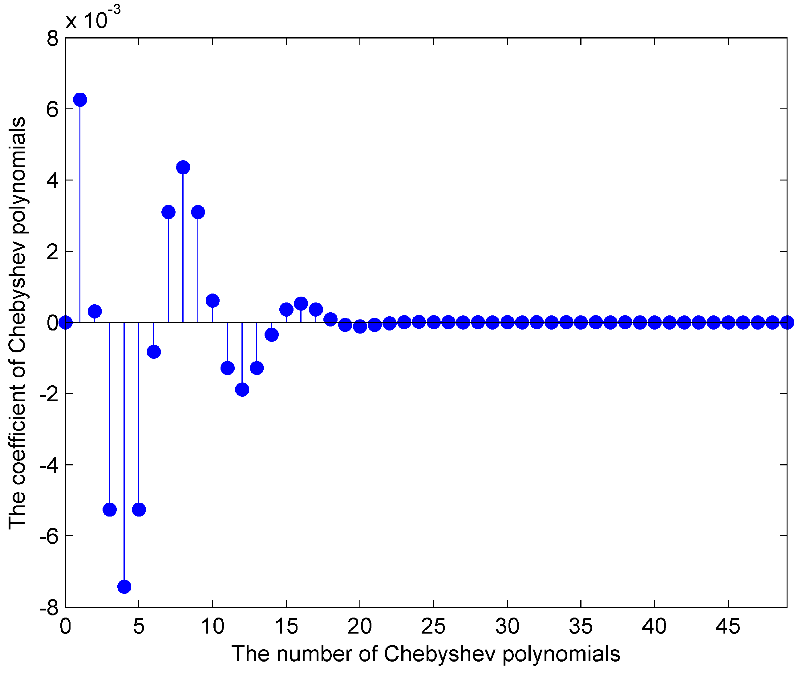
Figure 4 shows the coefficients of the first 50 Chebyshev polynomials. Figure 5 shows the reconstruction result of the Cook-Torrance model based on the first 20 coefficients and the Chebyshev polynomials.

As shown in Figure 5, the Cook-Torrance model can be reconstructed by using the first several items of Chebyshev polynomials. When the number of items is greater than 20, the curves in the x-coordinate range [0, 1] are not much different. The x-coordinate range [0, 1] is the range of incident angles in the experiment. When the Chebyshev polynomials involved in the reconstruction are less than 20 items, the reduction of the polynomials will reduce the accuracy of the reconstructed curve. However, the reduction of the items will increase the computing speed of compressive BRDF feature extraction at the same time. Although there are differences between the reconstructed curves and the original curve, the reconstructed curves can reflect the change trend of the original curve to some extent.

In this paper, we use a set of images with multiple illumination angles to extract the BRDF curves of the camouflaged object and background. The first several coefficients of the Chebyshev polynomials expansion on the BRDF curve are taken as the compressive BRDF feature. In the process of feature extraction, data loss is inevitable; however, the retained data can still reflect the difference between object and background.

3.2. Object Segmentation Based on the Compressive BRDF Feature

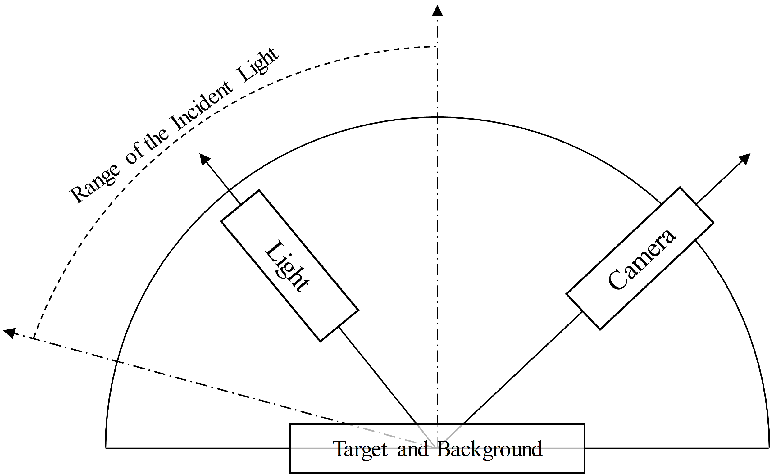
According to the above theory, the compressive BRDF feature can be extracted by multi-angle illumination images. The images can be taken by the experimental platform as shown in Figure 6.

As shown in Figure 6, the incident angle of light varies between 0${}^{\circ }$ and 76${}^{\circ }$, taking a point every 2${}^{\circ }$. The emergent angle is fixed as 45${}^{\circ }$. The incident light comes from an LED white light source. It is a broad-band source, whose energy is mainly in the wavelength from 450 nm to 500 nm. The divergence of the beam is about 120${}^{\circ }$. The camera is a single-channel camera with a focal length of 25 mm. The pixel size is 640 pixels × 512 pixels. By using this testing device, 39 images of the same scene can be obtained. The same pixel in each image corresponds to the same position on the object or background. The 39-dimensional grey-level feature of each pixel can be obtained.

By discretising Equations (15) and (16), the following formulas are obtained:

$$f_0=\frac{1}{\pi }\sum _{j=1}^{N-1}\left(\frac{f\left(x_j\right)}{\sqrt{1-x_j^2}}+\frac{f\left(x_{j+1}\right)}{\sqrt{1-x_{j+1}^2}}\right)\left(\frac{x_{j+1}-x_j}{2}\right)$$

(17)

$$f_n=\frac{2}{\pi }\sum _{j=1}^{N-1}\left(\frac{T\left(x_j\right)f\left(x_j\right)}{\sqrt{1-x_j^2}}+\frac{T\left(x_{j+1}\right)f\left(x_{j+1}\right)}{\sqrt{1-x_{j+1}^2}}\right)\left(\frac{x_{j+1}-x_j}{2}\right)$$

(18)

where N is the number of images; $f\left(x_j\right)$ represents the grey level of images; and $x_j$ denotes the input parameter of BRDF, expressed as

$$x_j=sin{\theta }_i=sin\left(\pi \ast \left(2\ast j-2\right)/180\right),j=1,2,\dots ,N$$

(19)

Equations (17) and (18) are used to perform the same processing on each pixel to obtain the low-dimensional compressed BRDF feature ${\left[f_0,f_1,\dots ,f_n\right]}_{3<n<14}$. By clustering the pixels into two categories, the camouflaged object and background are segmented. The steps of the proposed camouflaged object segmentation method are as follows in

Table 1. Steps of the proposed camouflaged object segmentation method.

Steps	Procedure
1	Take 39 images of the same scene with various incident angles ${\theta }_i$ of light and fix the emergent angle ${\theta }_r$ of the camera.
2	Extract the grey values from the images and obtain the 39-dimensional grey-level feature of each pixel.
3	Compress the 39-dimensional grey-level features into low-dimensional features by the Chebyshev polynomial expansion.
4	Cluster the compressive BRDF features of the pixels into two categories, one of which is the camouflaged object and the other one is background.

.

K-means clustering algorithm is an unsupervised clustering algorithm proposed by Mac Queen [27], which divides the dataset into K data subsets by minimising the error function. In this paper, the error function is expressed as

$$\epsilon =\sum _{r=1}^K\sum _{p\left(mm,nn\right)\in C_r}{\left|p\left(mm,nn\right)-q_r\right|}^2$$

(20)

where K = 2 denotes the number of clustering, $p\left(mm,nn\right)=\left[f_0,f_1,\dots ,f_n\right]{}_{\left(mm,nn\right)}$ represents the compressive BRDF feature of the pixel in row $mm$ and column $nn$, $C{}_r$ is the cluster of number r, and $q_r$ represents the central value of $C{}_r$.

4. Experiment and Analysis

4.1. Analysis of Feature Compression of Different Dimensions

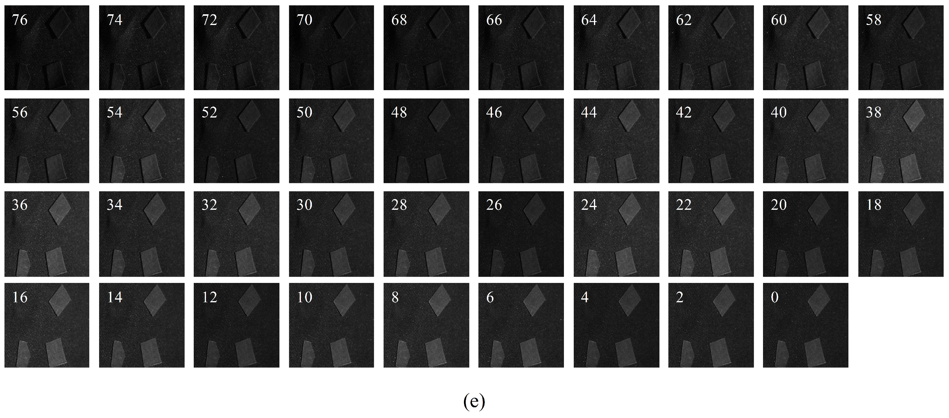
In order to verify that the low-dimensional compression of the multi-angle grey-level feature can achieve good effect in accuracy and running speed, the compressions of different dimensional features used in the camouflage object segmentation method are shown in this section. All the codes in this work are implemented by MATLAB 2012b on a PC with Intel i7-9700 CPU and 32.0 GB RAM. The program runs on one CPU core. There are five groups of original images, with 39 images in each group, as shown in Figure 7. In groups 1 to 4, the size of the single-channel grey images to be segmented is 250 pixels × 250 pixels, and the object and background are flat. The size of images in group 5 is 300 pixels × 300 pixels. In group 5, the top-left corner of the images has uneven folds. The central region of each image is the leaves, and the background is camouflaged cloth of the same colour.

In each diagram of Figure 7, from left to right and from top to bottom, the light incident angles range from 76${}^{\circ }$ to 0${}^{\circ }$ with an interval of 2${}^{\circ }$. As shown in Figure 7, in some images, the object and background can be easily distinguished by human eyes. However, in the other images, the grey values of the object and background are very close, leading to the difficulty of segmentation.

Figure 8 shows the effect of camouflaged object segmentation based on different dimensional compressive BRDF features.

As shown in Figure 8, from the first to the last row are the experimental results of groups 1 to 5. The first column shows the original images with the incident light of 44${}^{\circ }$. The second column is the ground truth images with the object position manually labelled. From the third to the eighth columns are the segmentation results based on different dimensional compressive BRDF features. In Figure 8, no matter the number of feature dimensions, the segmentation results of the objects are good. To evaluate the segmentation performance, the probability $P_d$ and the false alarm rate $F_a$ of the segmentation performance are defined as follows [28,29]:

$$P_d=\frac{N_{true}}{N_{actual}}$$

(21)

$$F_a=\frac{N_{false}}{w\times h}$$

(22)

where $N_{true}$ represents the pixel number of the true object area in the result images; $N_{actual}$ denotes the pixel number of the ground truth object; $N_{false}$ is the pixel number of the false object area in the result images; and w and h are the width and height of images, respectively. The probability and the false alarm rate of segmentation results based on different dimensional compressive BRDF features are shown in

Table 2. Probability and false alarm rate of segmentation results obtained by different dimensional features.

${\mathit{P}}_{\mathit{d}}$ (%)/${\mathit{F}}_{\mathit{a}}$ (%)	3	5	7	9	11	13
Group 1	90.50/45.44	89.30/42.18	89.54/44.49	89.57/45.18	91.74/47.30	85.39/44.19
Group 2	67.51/1.59	76.01/1.65	80.40/1.66	79.69/1.69	78.58/1.70	79.59/1.68
Group 3	96.94/33.57	96.73/29.88	96.87/21.06	96.95/30.36	96.68/22.10	96.94/30.48
Group 4	92.41/45.66	92.60/42.85	93.29/43.98	93.72/48.22	94.47/47.72	94.81/50.61
Group 5	73.11/32.24	73.50/32.77	74.01/33.77	74.23/34.16	71.98/30.62	74.41/34.86
Average	84.09/31.70	85.63/29.86	86.82/28.99	86.83/31.92	86.69/29.89	86.23/32.36

. In addition, the running time of the experiments, recorded by MATLAB’s built-in function, is shown in

Table 3. Running time of the proposed method obtained by different dimensional features.

Time (s)	3	5	7	9	11	13
Group 1	2.72	2.12	2.06	3.44	2.77	2.80
Group 2	2.75	1.36	2.74	2.05	2.07	2.08
Group 3	3.40	2.03	1.37	1.40	2.10	3.46
Group 4	2.05	2.05	1.40	3.48	1.38	2.80
Group 5	6.56	5.10	5.59	4.42	6.61	4.47
Average	3.49	2.53	2.63	2.96	2.99	3.12

.

As shown in Table 2 and Table 3, the difference in dimensions has little effect on the performance of the proposed compressive BRDF feature-based method. The running times of groups 1 to 4 are close to each other. Group 5 processed larger images than the first four groups; so, the running time is longer. Therefore, when comparing with other methods, we take the 7-dimensional compressive BRDF feature for the experiments.

4.2. Comparative Analysis of Different Camouflaged Object Segmentation Methods

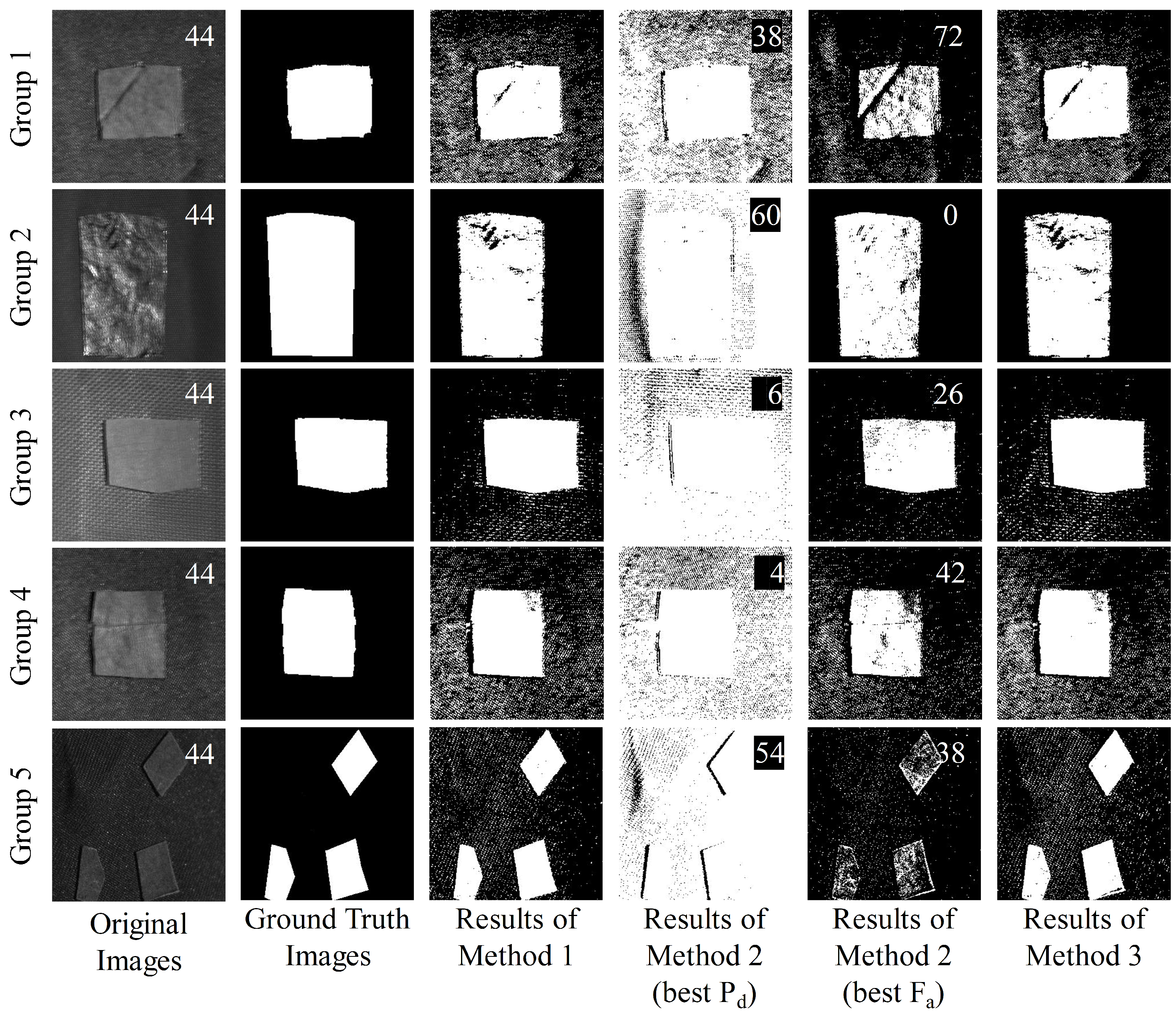
The comparisons between the compressive BRDF feature proposed in this paper, the grey-level feature used by Guo et al. [14], and the multi-dimensional grey-level feature constructed by Wang et al. [19] are conducted in this section. Method 1 is a clustering method using the 7-dimensional compressive BRDF features proposed in this paper. Method 2 uses the 1-dimensional grey feature for clustering. Method 3 uses the 39-dimensional grey-level feature for clustering. The performance of the three methods is shown in Figure 9.

In Figure 9, each row shows the result images of each group obtained by the three methods. The first and second column are the original images and the ground truth images. The third column shows the results images achieved by Method 1. All the images in Figure 6 are segmented using Method 2, with the fourth column showing the result images with the highest probability $P_d$ and the fifth column showing the result images with the lowest false alarm rate $F_a$. The numbers on them represent the incident light angle of original images. The sixth column indicates the result images obtained by Method 3. As shown in Figure 8, the performance of Method 2 is unstable, which means that the result images are easily affected by the incident light angle. The performance of Method 3 is better than that of Method 2 and close to Method 1. However, it needs more running time. The probability and false alarm rate of the segmentation results obtained by the three methods are shown in

Table 4. Probability and false alarm rate of segmentation results obtained by the three methods.

${\mathit{P}}_{\mathit{d}}$ (%)/${\mathit{F}}_{\mathit{a}}$ (%)	Method 1 (7D)	Method 2 (Best ${\mathit{P}}_{\mathit{d}}$)	Method 2 (Best ${\mathit{F}}_{\mathit{a}}$)	Method 2 (Average)	Method 3
Group 1	89.54/44.49	96.53/64.37	39.69/22.26	79.47/51.58	88.83/39.96
Group 2	80.40/1.66	96.55/50.41	35.26/1.33	67.45/20.71	76.33/1.67
Group 3	96.87/21.06	98.56/69.76	59.86/16.14	81.68/56.19	96.70/22.61
Group 4	93.29/43.98	98.05/76.37	66.21/33.25	80.13/58.67	92.22/40.03
Group 5	74.01/33.77	89.17/80.14	15.82/21.54	60.91/54.34	70.40/36.69
Average	86.82/28.99	95.77/68.21	43.37/18.90	73.93/48.30	84.90/28.19

. The running times of the experiments are shown in

Table 5. Running time of the proposed method obtained by the three methods.

Time (s)	Method 1 (7D)	Method 2 (Best ${\mathit{P}}_{\mathit{d}}$)	Method 2 (Best ${\mathit{F}}_{\mathit{a}}$)	Method 2 (Average)	Method 3
Group 1	2.06	0.19	0.35	0.24	3.62
Group 2	2.74	0.17	0.35	0.24	2.88
Group 3	1.37	0.17	0.17	0.23	5.97
Group 4	1.40	0.18	0.35	0.21	2.17
Group 5	5.59	0.50	0.70	0.56	8.30
Average	2.63	0.24	0.39	0.30	4.59

.

As shown in Table 4, compared with Method 2, the probability of segmentation achieved by Method 1 is more stable. Regardless of the result images with the highest probability or the lowest false alarm rate, the visual segmentation effect is not as good as method 1. Compared with Method 2, the probability of the proposed method is improved by 17.44% and the false alarm rate is reduced by 39.98%. Compared with Method 3, the probability of segmentation is improved by 2.26%, with the false alarm rate slightly higher. As shown in Table 5, the running time of Method 1 is reduced by 42.70% compared with Method 3. In conclusion, compared with one-dimensional and multi-dimensional grey-level features, the comprehensive performance of the presented compressive BRDF feature for camouflaged object segmentation methods has remarkable advantages.

4.3. Comparison of Performance for Methods Based on Grey Images

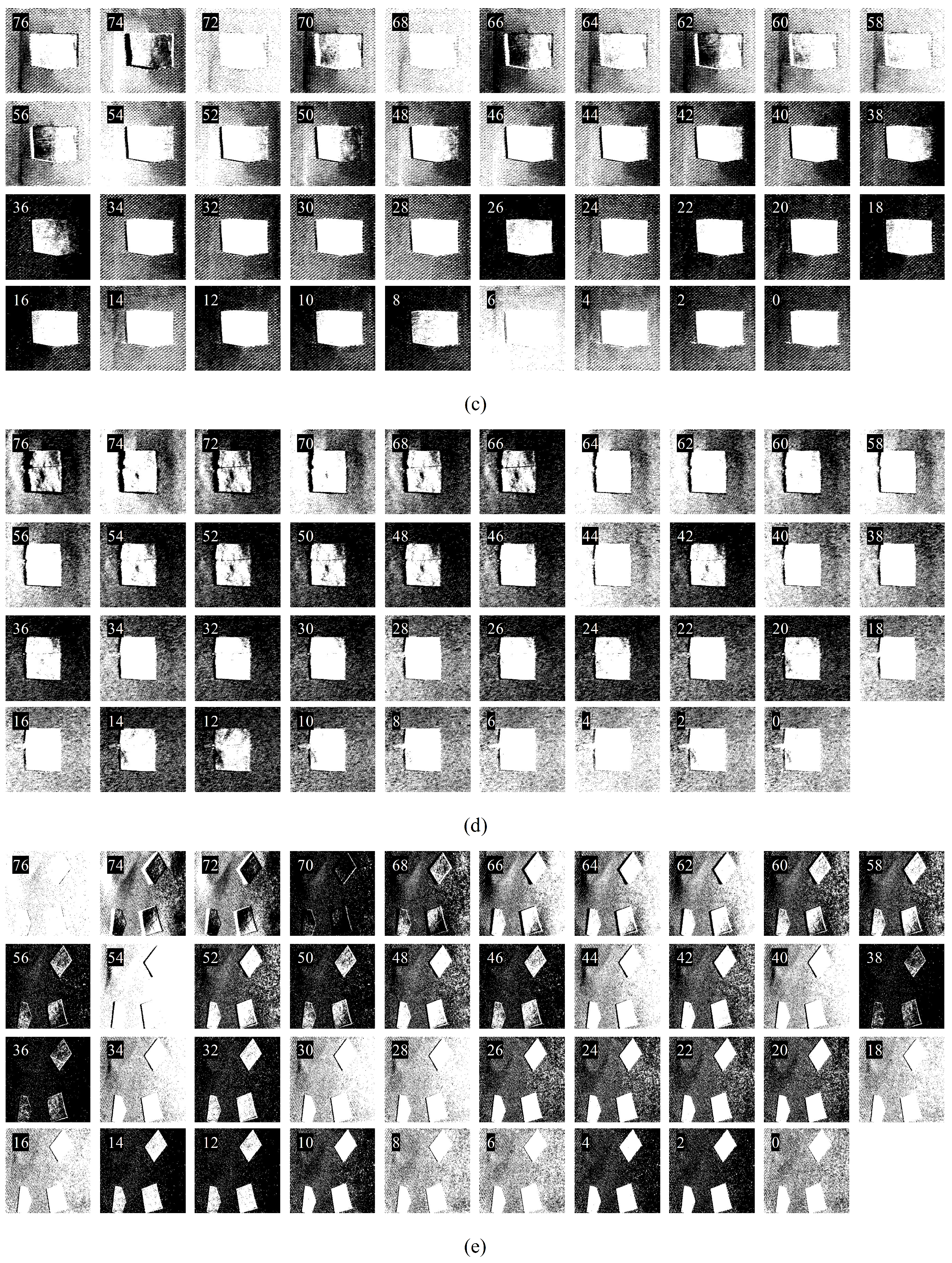
In Section 4.2, we compare the result images obtained by Method 1 with the best-performance result images obtained by Method 2. However, the highest probability and the lowest false alarm rate do not occur in the same resulting image. A detailed comparison of performance between the proposed Method 1 and Method 2 based on one-dimensional grey-level feature is shown in this section. The result images obtained by Method 2 are shown in Figure 10.

In each diagram of Figure 10, from left to right and from top to bottom, the light incident angles are from 76${}^{\circ }$ to 0${}^{\circ }$. As shown in Figure 10, the segmentation effect is unstable. The probability and false alarm rate of segmentation results obtained by the three methods are shown in

Table 6. Probability and false alarm rate of segmentation results obtained by Method 2.

${\mathit{P}}_{\mathit{d}}$ (%)/${\mathit{F}}_{\mathit{a}}$ (%)	Group 1	Group 2	Group 3	Group 4	Group 5	Average
76${}^{\circ }$	86.83/71.76	84.53/27.08	93.91/71.24	59.52/76.19	87.93/81.40	82.54/65.53
74${}^{\circ }$	76.83/55.33	95.45/47.63	93.85/69.51	35.76/47.52	20.44/63.26	64.47/56.65
72${}^{\circ }$	67.87/38.10	84.06/23.79	42.18/64.61	55.67/51.22	14.99/60.96	52.96/47.74
70${}^{\circ }$	77.90/51.18	87.41/29.66	93.37/70.47	41.91/41.06	4.76/33.32	61.07/45.14
68${}^{\circ }$	47.16/31.06	84.66/26.89	32.68/62.17	64.95/57.50	24.47/46.55	50.78/44.83
66${}^{\circ }$	58.17/30.06	87.95/30.89	94.79/73.28	50.25/77.34	64.85/64.05	71.20/55.12
64${}^{\circ }$	39.69/22.26	96.55/50.41	57.10/64.69	49.04/37.47	67.37/65.15	61.95/47.99
62${}^{\circ }$	81.28/51.84	67.78/17.89	68.95/62.87	96.92/67.84	71.90/66.40	77.36/53.37
60${}^{\circ }$	89.93/63.44	84.66/34.12	77.04/66.65	95.83/60.12	42.93/49.57	78.08/54.78
58${}^{\circ }$	42.40/24.33	68.63/29.22	37.57/57.38	97.71/72.80	47.30/50.06	58.72/46.76
56${}^{\circ }$	82.08/41.95	61.07/32.03	74.70/69.00	94.53/66.14	21.24/35.77	66.72/48.98
54${}^{\circ }$	92.86/58.38	48.02/32.80	66.79/72.28	56.62/42.43	89.17/80.14	70.69/57.20
52${}^{\circ }$	91.65/53.80	46.16/39.52	67.49/65.68	98.05/76.37	60.78/50.99	72.83/57.27
50${}^{\circ }$	56.62/29.77	48.32/54.40	65.04/63.52	87.40/56.08	29.44/36.16	57.36/47.99
48${}^{\circ }$	88.97/58.73	31.24/28.00	83.35/56.68	97.46/60.19	65.54/51.69	73.31/51.06
46${}^{\circ }$	83.03/52.08	74.25/50.76	97.63/71.93	96.46/54.22	33.52/36.46	76.98/53.09
44${}^{\circ }$	91.43/48.66	82.26/40.79	81.02/48.40	97.23/59.34	82.50/71.51	86.89/53.74
42${}^{\circ }$	94.61/66.11	85.78/28.88	97.30/67.71	97.16/59.41	71.88/52.39	89.35/54.90
40${}^{\circ }$	93.27/63.75	60.87/1.68	34.33/36.06	97.38/67.89	82.94/72.22	73.76/48.32
38${}^{\circ }$	93.65/63.30	67.73/2.28	96.25/48.08	92.78/54.11	15.82/21.54	73.24/37.86
36${}^{\circ }$	81.38/39.35	72.80/1.62	97.22/64.67	97.70/70.42	16.70/21.72	73.16/39.56
34${}^{\circ }$	89.31/56.16	71.09/1.67	96.59/43.23	97.23/57.77	82.95/72.86	87.43/46.34
32${}^{\circ }$	94.58/54.06	72.93/1.77	59.86/16.14	85.02/36.03	46.51/37.35	71.78/29.07
30${}^{\circ }$	94.82/64.40	54.20/1.47	96.63/47.12	97.13/65.57	83.67/73.51	85.29/50.41
28${}^{\circ }$	60.37/45.14	57.70/1.52	96.60/29.17	66.21/33.25	83.55/73.62	72.89/36.54
26${}^{\circ }$	91.16/47.09	76.31/2.25	96.91/54.07	96.51/51.57	76.88/52.68	87.55/41.53
24${}^{\circ }$	96.53/64.37	71.79/1.61	96.56/34.95	96.70/63.27	76.00/52.37	87.51/43.31
22${}^{\circ }$	55.06/34.96	76.73/1.67	94.37/40.27	97.64/67.66	76.77/51.67	80.12/39.25
20${}^{\circ }$	92.95/52.38	65.06/1.58	97.91/71.13	90.39/59.51	77.07/51.12	84.68/47.14
18${}^{\circ }$	93.07/53.23	35.26/1.33	97.09/47.73	97.62/70.25	85.16/73.37	81.64/49.18
16${}^{\circ }$	67.45/44.01	63.39/2.81	97.06/61.37	97.56/67.76	85.03/73.08	82.10/49.81
14${}^{\circ }$	82.14/50.76	36.98/1.89	92.01/38.38	53.10/42.06	53.11/30.77	63.47/32.77
12${}^{\circ }$	94.87/69.83	32.60/3.67	97.95/59.24	55.75/58.14	49.99/30.40	66.23/44.26
10${}^{\circ }$	83.71/54.30	32.87/40.92	97.70/63.58	70.18/47.50	77.54/45.94	72.4/50.45
8${}^{\circ }$	87.90/59.33	59.96/55.16	97.17/47.29	95.07/58.72	84.10/70.22	84.84/58.14
6${}^{\circ }$	48.03/46.04	52.04/3.35	98.56/69.76	77.14/51.62	83.65/69.29	71.88/48.01
4${}^{\circ }$	72.76/56.44	86.54/45.15	67.35/45.64	67.46/62.66	76.78/42.27	74.18/50.43
2${}^{\circ }$	88.09/71.36	73.19/2.44	55.37/32.73	68.51/75.63	76.93/40.82	72.42/44.60
0${}^{\circ }$	89.06/72.56	91.67/7.26	97.14/62.66	55.55/63.36	83.54/66.73	83.39/54.51
Average	79.47/51.58	67.45/20.71	81.68/56.19	80.13/58.67	60.91/54.34	73.93/48.30

.

We compare the performance data of result images obtained by Method 2 with the performance data in the second column of Table 4 in Section 4.2. The result of the comparison is shown in

Table 7. Comparison of the performance of Method 1 and Method 2.

Number	Group 1	Group 2	Group 3	Group 4	Group 5	Average
$P_d$: Method 1 > Method 2.	25	27	27	20	20	23.8
$F_a$: Method 1 < Method 2.	29	33	38	33	34	33.4

.

As shown in Table 6 and Table 7, compared with Method 2, the result images of Method 1 are higher in the probability than 61.03% of the result images obtained by Method 2. The false alarm rate of Method 1 is lower than 85.64% of the result images obtained by Method 2. No result images can be better than Method 1 on both performances. The running times of the experiments are shown in

Table 8. Running time of the segmentation results obtained by Method 2.

Time (s)	Group 1	Group 2	Group 3	Group 4	Group 5	Average
76${}^{\circ }$	0.18	0.18	0.18	0.17	0.57	0.26
74${}^{\circ }$	0.18	0.18	0.17	0.17	0.71	0.28
72${}^{\circ }$	0.18	0.18	0.18	0.18	0.58	0.26
70${}^{\circ }$	0.35	0.18	0.18	0.18	0.59	0.29
68${}^{\circ }$	0.18	0.17	0.17	0.18	0.75	0.29
66${}^{\circ }$	0.17	0.17	0.18	0.17	0.66	0.27
64${}^{\circ }$	0.35	0.17	0.35	0.18	0.69	0.35
62${}^{\circ }$	0.35	0.18	0.17	0.18	0.65	0.31
60${}^{\circ }$	0.18	0.18	0.17	0.18	0.50	0.24
58${}^{\circ }$	0.36	0.18	0.17	0.18	0.48	0.27
56${}^{\circ }$	0.17	0.17	0.18	0.18	0.50	0.24
54${}^{\circ }$	0.18	0.18	0.18	0.18	0.50	0.24
52${}^{\circ }$	0.17	0.18	0.18	0.18	0.56	0.25
50${}^{\circ }$	0.35	0.17	0.18	0.18	0.54	0.28
48${}^{\circ }$	0.18	0.17	0.18	0.35	0.51	0.28
46${}^{\circ }$	0.36	0.17	0.36	0.18	0.54	0.32
44${}^{\circ }$	0.17	0.18	0.17	0.35	0.53	0.28
42${}^{\circ }$	0.18	0.18	0.17	0.18	0.84	0.31
40${}^{\circ }$	0.36	0.35	0.35	0.18	0.77	0.40
38${}^{\circ }$	0.36	0.52	0.18	0.37	0.70	0.43
36${}^{\circ }$	0.36	0.18	0.18	0.18	0.52	0.28
34${}^{\circ }$	0.18	0.53	0.17	0.17	0.58	0.33
32${}^{\circ }$	0.18	0.53	0.17	0.35	0.51	0.35
30${}^{\circ }$	0.18	0.35	0.18	0.36	0.51	0.31
28${}^{\circ }$	0.37	0.35	0.35	0.35	0.48	0.38
26${}^{\circ }$	0.19	0.18	0.35	0.18	0.49	0.28
24${}^{\circ }$	0.19	0.53	0.35	0.18	0.52	0.35
22${}^{\circ }$	0.37	0.17	0.35	0.18	0.46	0.31
20${}^{\circ }$	0.37	0.53	0.18	0.17	0.49	0.35
18${}^{\circ }$	0.18	0.35	0.35	0.35	0.49	0.34
16${}^{\circ }$	0.35	0.18	0.18	0.18	0.53	0.28
14${}^{\circ }$	0.18	0.18	0.35	0.18	0.48	0.27
12${}^{\circ }$	0.17	0.17	0.35	0.18	0.54	0.28
10${}^{\circ }$	0.18	0.17	0.18	0.18	0.52	0.25
8${}^{\circ }$	0.17	0.18	0.18	0.18	0.65	0.27
6${}^{\circ }$	0.35	0.18	0.17	0.18	0.51	0.28
4${}^{\circ }$	0.17	0.18	0.35	0.18	0.44	0.26
2${}^{\circ }$	0.18	0.18	0.35	0.18	0.50	0.28
0${}^{\circ }$	0.18	0.35	0.18	0.18	0.41	0.26
Average	0.18	0.18	0.18	0.17	0.57	0.26

.

As shown in Table 6, Table 7 and Table 8, although Method 2, which is based on a one-dimensional grey-level feature, is fast on computing speed, Method 1 is better than Method 2 on its performances of probability and false alarm rate.

5. Conclusions

5.1. Summary of Our Method

In this paper, a compressive BRDF-based feature extraction method for camouflaged object segmentation is proposed. First, multidimensional grey-level features are extracted from multiple images with different illumination incident angles in the same scene. Then, we conduct the Chebyshev polynomials expansion on the multidimensional grey-level features. Next, we use the first several coefficients as a new feature, which is named the compressive BRDF feature. Finally, by clustering the compressive BRDF feature of each pixel, the camouflaged object is segmented from the background. Both qualitative and quantitative experimental results verify that the comprehensive performance of the presented camouflaged object segmentation method has remarkable advantages over conventional methods.

5.2. Limitations

The proposed method has some limitations. It is suitable for situations where the multi-dimensional grey-level features of the camouflaged object can be extracted. However, it cannot be used in instances where the camouflaged object is in an image with a fixed illumination angle and a fixed shooting angle. In addition, the false alarm rate of the presented method needs to be further reduced by improving the method.

5.3. Application Discussion

The proposed method can be applied in drone reconnaissance, when the detector appears in the same location at multiple times. In this application, image registration is required before segmentation. Another application is the detection of large camouflaged targets on the ground using geostationary satellites. In this condition, the loss of light intensity in the atmospheric transport needs to be considered. The proposed method is still in the stage of theoretical research, and further study is needed for practical application.

References

1. Shinde, R.C.; Jibu, M.C.; Patil, C. Segmentation Technique for Soybean Leaves Disease Detection. Int. J. Adv. Res. 2015, 5, 522–528. [Google Scholar]
2. Bukhari, H.R.; Mumtaz, R.; Inayat, S.; Shafi, U.; Haq, I.U.; Zaidi, S.M.H.; Hafeez, M. Assessing the Impact of Segmentation on Wheat Stripe Rust Disease Classification Using Computer Vision and Deep Learning. IEEE Access 2021, 9, 164986–165004. [Google Scholar] [CrossRef]
3. Patil, R.; Hegadi, R.S. Segmrntation on cotton insects and pests using image processing. In Proceedings of the National Conference on Current Trends in Advanced Computing and e-Learning, Uttar Pradesh, India, 6–7 October 2009. [Google Scholar]
4. Yan, J.; Le, T.; Nguyen, K.; Tran, M.; Do, T.; Nguyen, T.V. MirrorNet: Bio-Inspired Camouflaged Object Segmentation. IEEE Access 2021, 9, 43290–43300. [Google Scholar] [CrossRef]
5. Chowdhury, T.; Rahnemoonfar, M. Attention based semantic segmentation on UAV dataset for natural disaster damage assessment. In Proceedings of the IEEE International Geoscience and Remote Sensing Symposium, Brussels, Belgium, 11–16 July 2021. [Google Scholar]
6. Ren, Y.; Liu, Y. Geological disaster detection from remote sensing image based on experts’ knowledge and image features. In Proceedings of the IEEE International Geoscience and Remote Sensing Symposium, Beijing, China, 10–15 July 2016. [Google Scholar]
7. Ji, Z.; Meng, X. Automatic Identification of Targets Detected by Battlefield Scout Ragar. J. Harbin Inst. Technol. 2011, 33, 830–833. (In Chinese) [Google Scholar]
8. Wan, M.; Gu, G.; Qian, W.; Ren, K.; Chen, Q. Stokes-vector-based Polarimetric Imaging System for Adaptive Target/Background Contrast Enhancement. Appl. Opt. 2016, 55, 5513–5519. [Google Scholar] [CrossRef] [PubMed]
9. Xu, X.; Wan, M.; Ge, J.; Chen, H.; Zhu, X.; Zhang, X.; Chen, Q.; Gu, G. ColorPolarNet: Residual Dense Network-Based Chromatic Intensity-Polarization Imaging in Low Light Environment. IEEE Trans. Instrum. Meas. 2022, 71, 5025210. [Google Scholar] [CrossRef]
10. Goccia, M.; Bruzzo, M.; Scagliola, C.; Dellepiane, S. Recognition of container code characters through gray–level feature extraction and gradient–based classifier optimization. In Proceedings of the International Conference on Document Analysis & Recognition, Edinburgh, UK, 3–6 August 2003. [Google Scholar]
11. Zhao, J.; Liu, M.; Yang, G. Discrimination of Mature Tomato Based on HIS Color Space in Natural Outdoor Scenes. Trans. Chin. Soc. Agric. Mach. 2004, 35, 122–125. (In Chinese) [Google Scholar]
12. Zheng, L.; Zhang, J.; Wang, Q. Mean-shift-based Color Segmentation of Images Containing Green Vegetation. Comput. Electron. Agric. 2009, 65, 93–98. [Google Scholar] [CrossRef]
13. Chen, J.; Zhu, S.; Cui, H.; Cui, P. Automated Crater Detection Method Using Gray Value Features and Planet Landing Navigation Research. J. Astronaut. 2014, 35, 908–915. (In Chinese) [Google Scholar]
14. Guo, C.; Wang, X.; Shi, C.; Jin, H. Corn Leaf Image Segmentation Based on Improved Kmeans Algorithm. J. North Univ. China (Nat. Sci. Ed.) 2021, 42, 524–529. (In Chinese) [Google Scholar]
15. Liu, X. Multi-Angle Identification of Potato Late Blight Based on Multi-Spectral Imaging. Master’s Thesis, Yunnan Normal University, Kunming, China, 7 June 2017. (In Chinese). [Google Scholar]
16. Yan, Y.; Hua, W.; Zhang, Y.; Cui, Z.; Wu, X.; Liu, X. Hyperspectral camouflage object characteristic analysis. In Proceedings of the International Symposium on Advanced Optical Manufacturing and Testing Technologies: Optoelectronic Materials and Devices for Sensing and Imaging, Chengdu, China, 8 February 2019. [Google Scholar]
17. Yang, Y. Bearing Surface Defect Detection System Based on Multi-Angle Light Source Image. Master’s Thesis, Dalian University of Technology, Dalian, China, 3 June 2019. (In Chinese). [Google Scholar]
18. Wu, J. Research on Textiles Color Segmentation and Extraction Based on Hyperspectral Imaging Technology. Master’s Thesis, Zhejiang Sci-Tech University, Hangzhou, China, 24 December 2019. (In Chinese). [Google Scholar]
19. Wang, C.; Chen, W.; Lu, C.; Wang, Q. Segmentation Method for Maize Stubble Row Based on Hyperspectral Imaging. Trans. Chin. Soc. Agric. Mach. 2020, 51, 421–426. (In Chinese) [Google Scholar]
20. Wang, O.; Gunawardane, P.; Scher, S.; Davis, J. Material classification using BRDF slices. In Proceedings of the IEEE Conference on Computer Vision and Pattern Recognition, Miami, FL, USA, 20–25 June 2009. [Google Scholar]
21. Skaff, S. Material Classification Using BRDF Slices. U.S. Patent US2015/0012226 A1, 8 January 2015. [Google Scholar]
22. Zhao, H.; Nie, F.; Tao, H. Study on BRDF Feature Model of Rock Surface. J. Hubei Univ. Arts Sci. 2015, 36, 481–502. (In Chinese) [Google Scholar]
23. Nicodemus, F. Directional Reflectance and Emissivity of an Opaque Surface. Appl. Opt. 1965, 4, 767–773. [Google Scholar] [CrossRef]
24. Cook, R.; Torrance, K. A Reflectance Models for Computer Graphics. ACM Trans. Graph. 1982, 1, 7–24. [Google Scholar] [CrossRef]
25. Revers, M. On the Asymptotics of Polynomial Interpolation to x α at the Chebyshev Nodes. J. Approx. Theory 2013, 165, 70–82. [Google Scholar] [CrossRef] [Green Version]
26. Zhang, X.; Li, J.; Zhang, Z. Distribution of a Sequence of Chebyshev Polynomials. Math. Pract. Theory 2022, 52, 276–280. (In Chinese) [Google Scholar]
27. Anzai, Y. Pattern Recognition and Machine Learning; Elsevier: Amsterdam, The Netherlands, 2012. [Google Scholar]
28. Rivest, J. Detection of Dim Targets in Digital Infrared Imagery by Morphological Image Processing. Opt. Eng. 1996, 35, 1886–1893. [Google Scholar] [CrossRef]
29. Gao, C.; Meng, D.; Yang, Y.; Wang, Y.; Zhou, X.; Hauptmann, A.G. Infrared Patch-Image Model for Small Object Detection in a Single Image. IEEE Trans. Image Process. 2013, 22, 4996–5009. [Google Scholar] [CrossRef] [PubMed]
Figure 1. Diagram of the light angles in BRDF model.
Photonics 09 00915 g001
Figure 2. Diagram of the reflection process.
Photonics 09 00915 g002
Figure 3. Diagram of the Cook-Torrance model (reflectance vs. incident angle).
Photonics 09 00915 g003
Figure 4. Diagram of the coefficients of Chebyshev polynomial expansion.
Photonics 09 00915 g004
Figure 5. Diagram of the theory and reconstruction of the Cook-Torrance model.
Photonics 09 00915 g005
Figure 6. Diagram of the BRDF model measuring equipment.
Photonics 09 00915 g006
Figure 7. Diagram of all the images to be segmented: (a) Group 1; (b) Group 2; (c) Group 3; (d) Group 4; (e) Group 5. Note that the incident angles of light are marked on the images.
Photonics 09 00915 g007aPhotonics 09 00915 g007b
Figure 8. Diagram of the segmentation result images achieved by different dimensional features.
Photonics 09 00915 g008
Figure 9. Diagram of the segmentation result images. Note that the incident angles of light are marked on the original images and the result images of Method 2.
Photonics 09 00915 g009
Figure 10. Diagram of the segmentation result images obtained by Method 2: (a) Group 1; (b) Group 2; (c) Group 3; (d) Group 4; (e) Group 5. Note that the incident angles of light are marked on the images.
Photonics 09 00915 g010aPhotonics 09 00915 g010b