TSC-1 Optical Payload Hyperspectral Imager Preliminary Design and Performance Estimation

 , , ,
, , ,
Abstract
:1. Introduction
1.1. TSC-1 Mission, Context and Impact on Technical Choices
1.2. TSC-1 Payload Scientific Objectives and Specifications
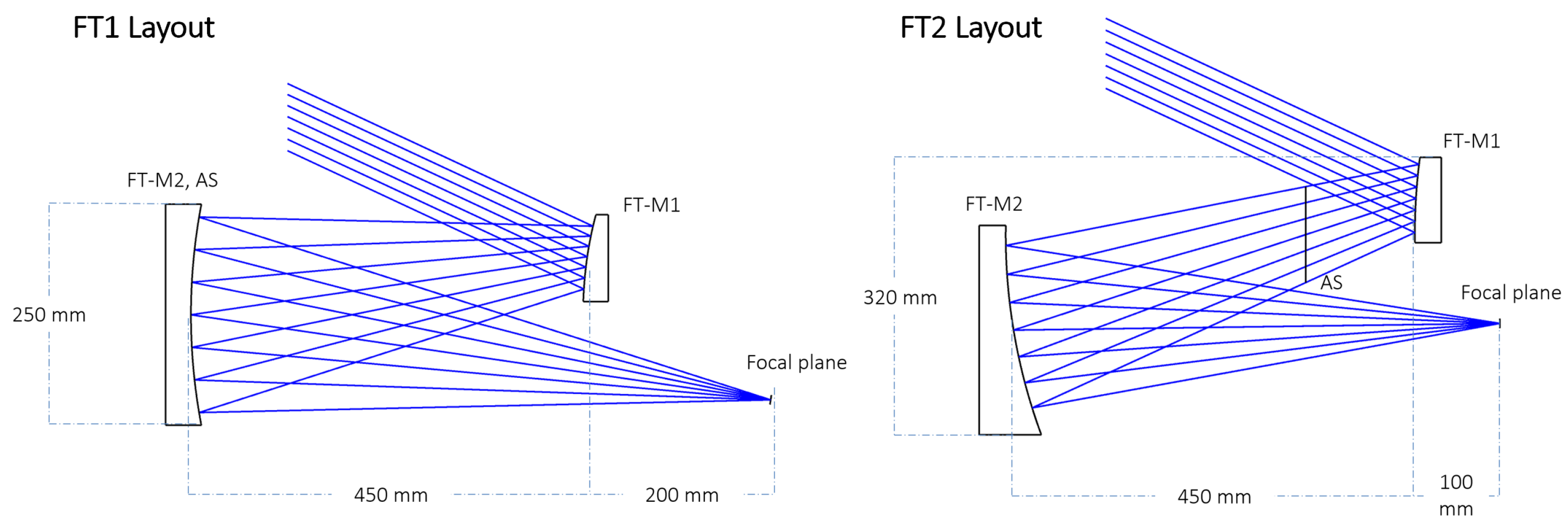
2. Front Telescope Design Trade-Off
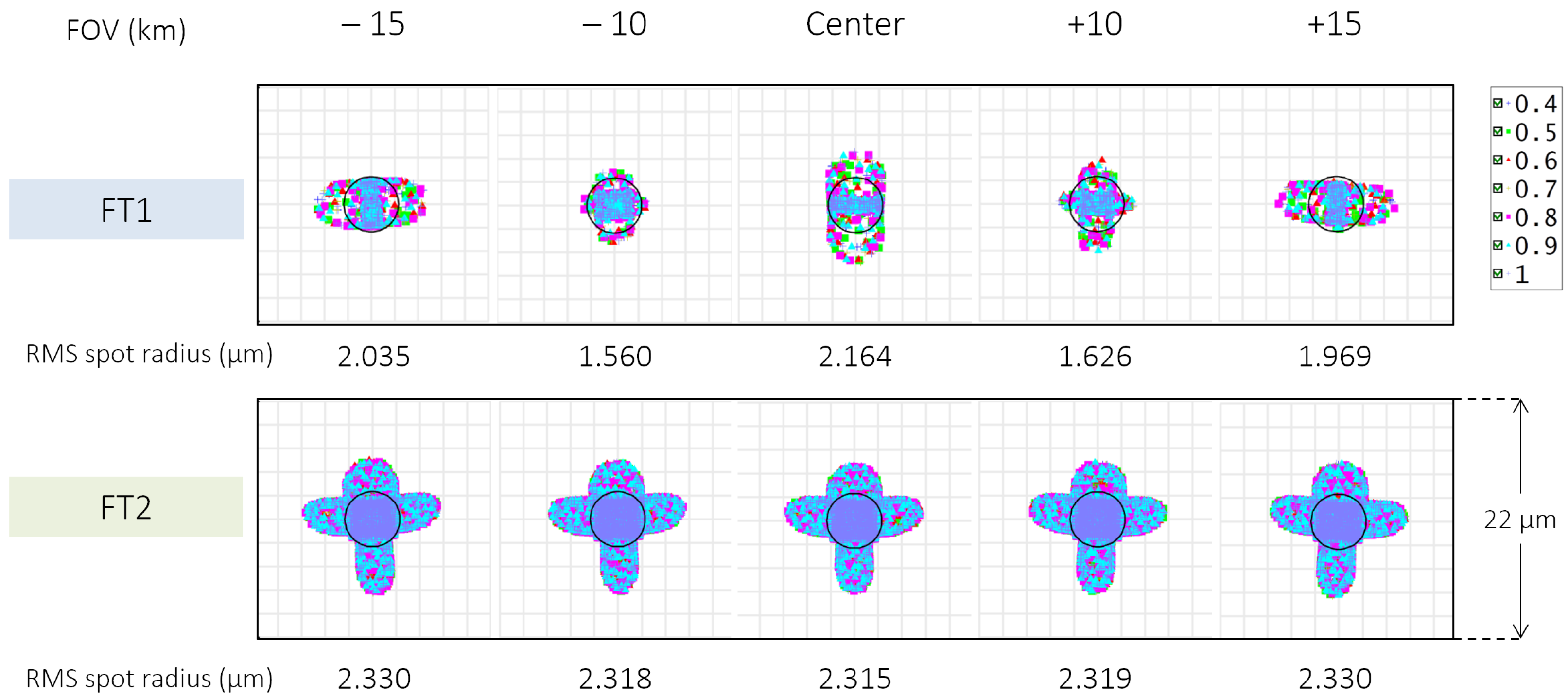
2.1. Optical Design and Theoretical Performance
2.2. Sensitivity Matrix
2.3. Front Telescope Design Selection
3. Spectrometer Design Trade-Off
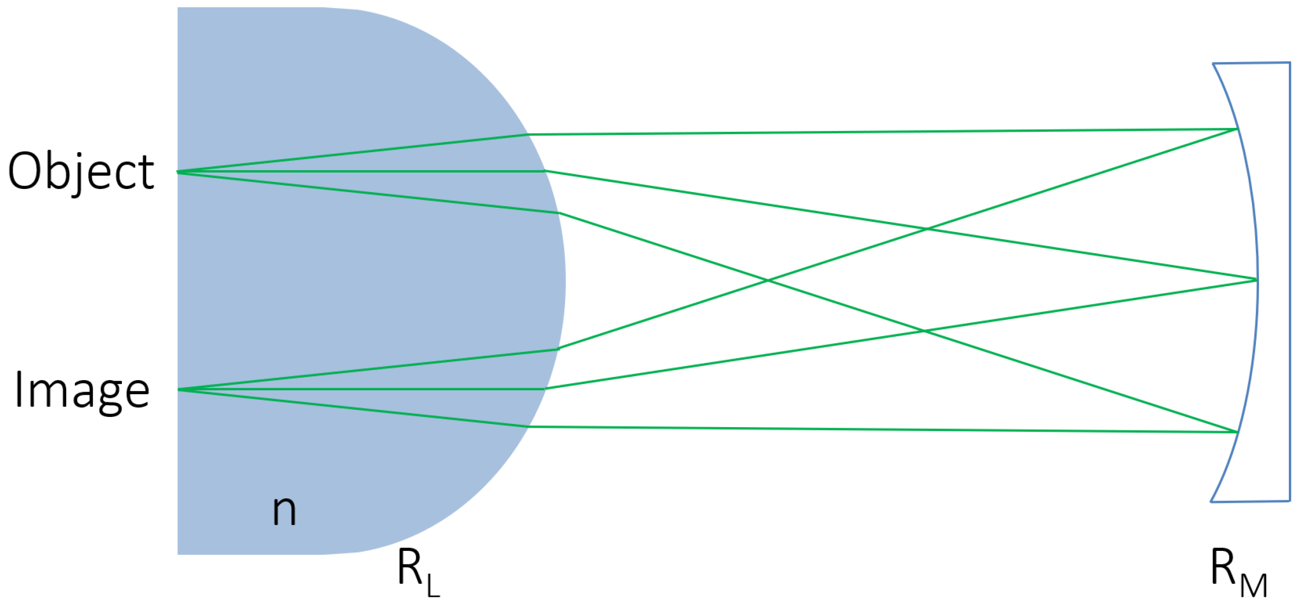
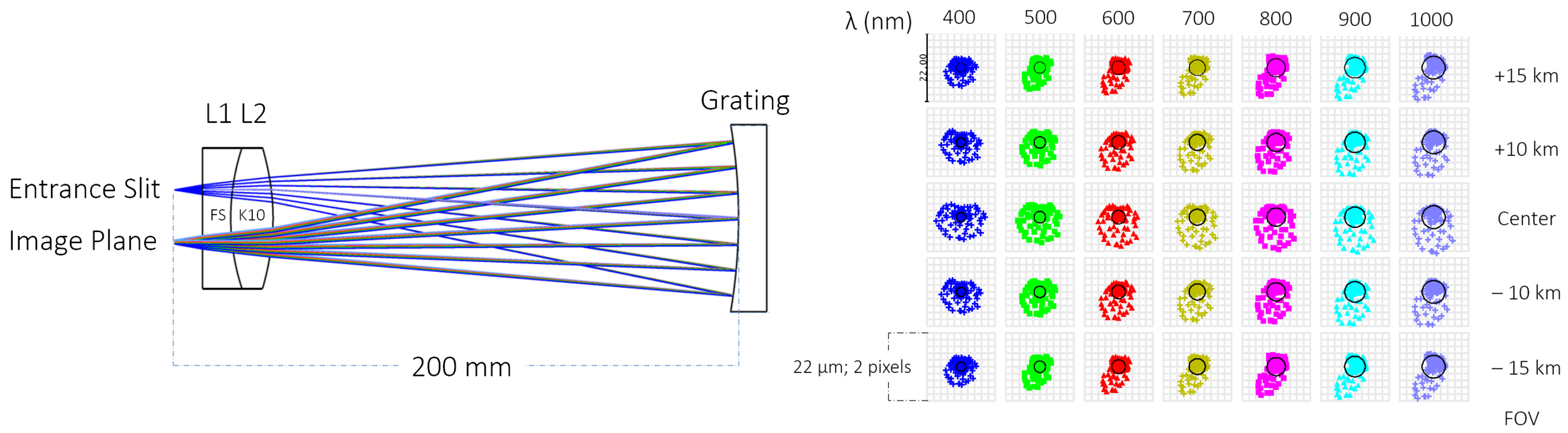
3.1. Dyson Spectrometer Design
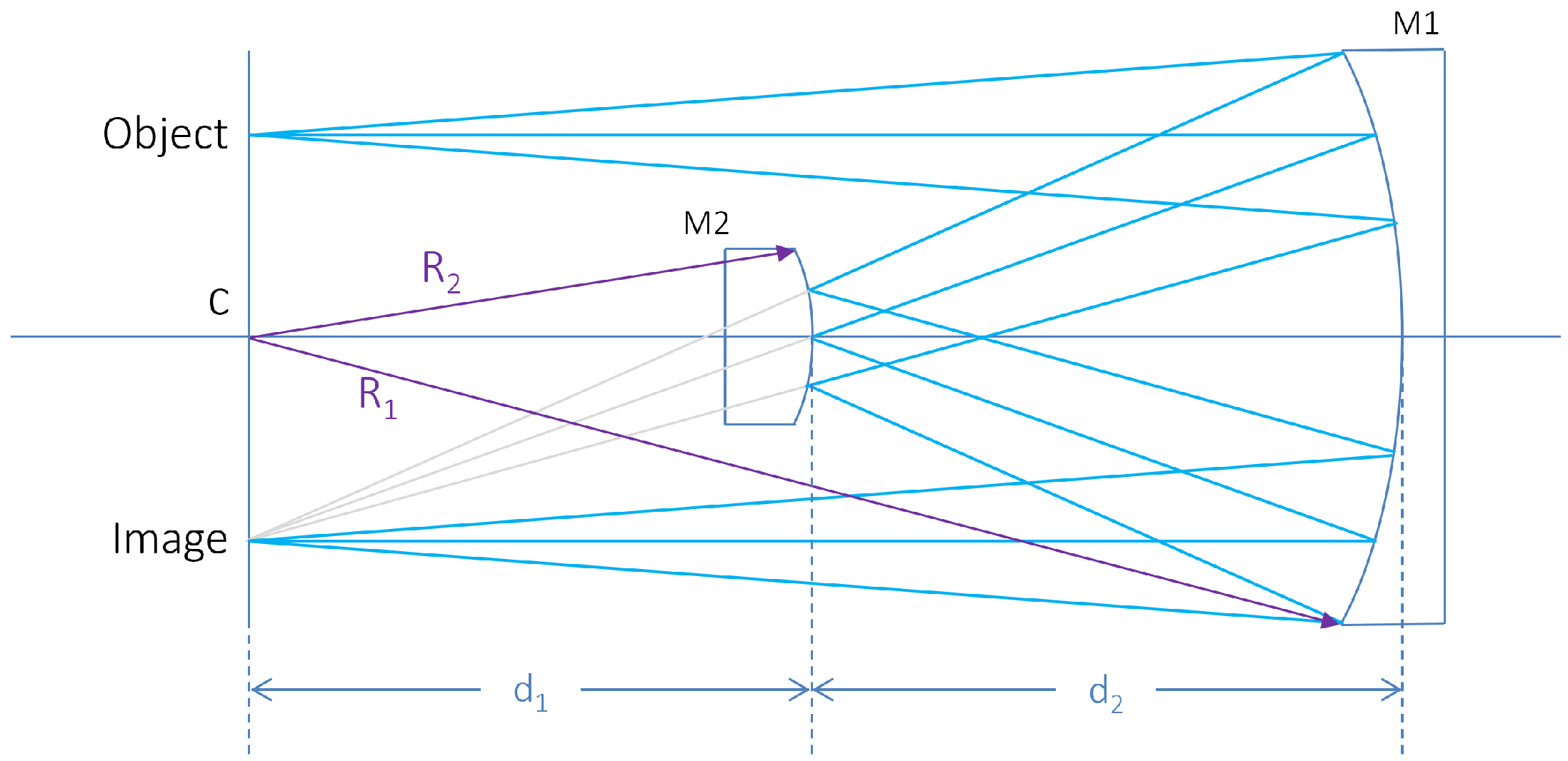
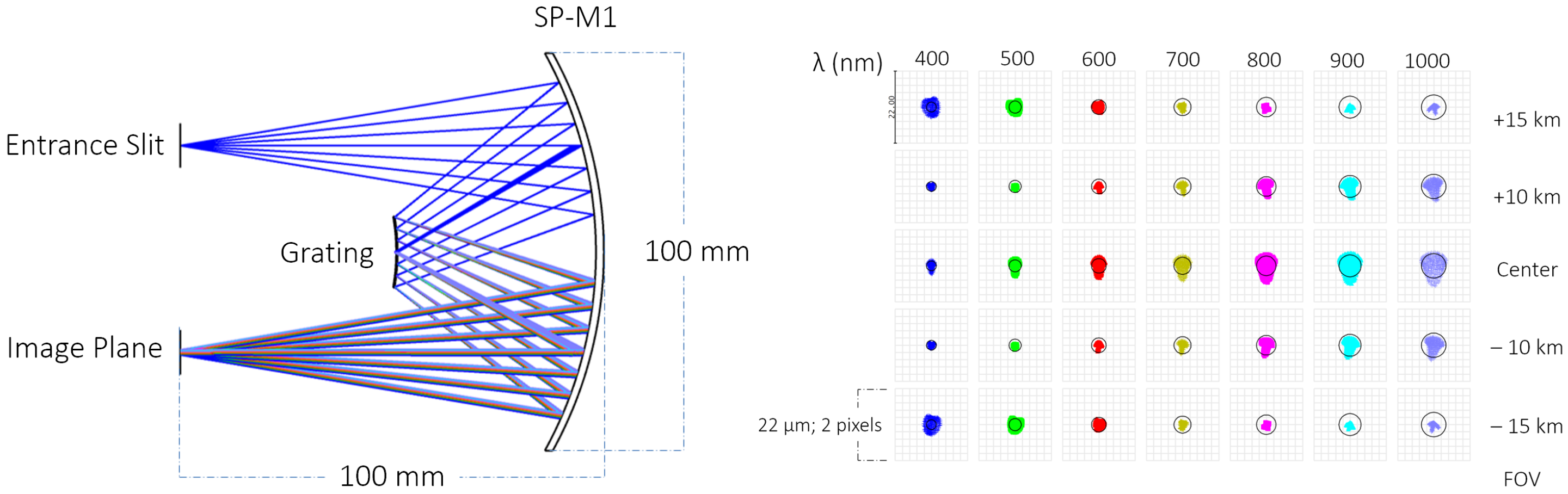
3.2. Offner Spectrometer Design
3.3. Trade Off and Design Selection
4. TSC-1 Payload Optical Design and Theoretical Performance
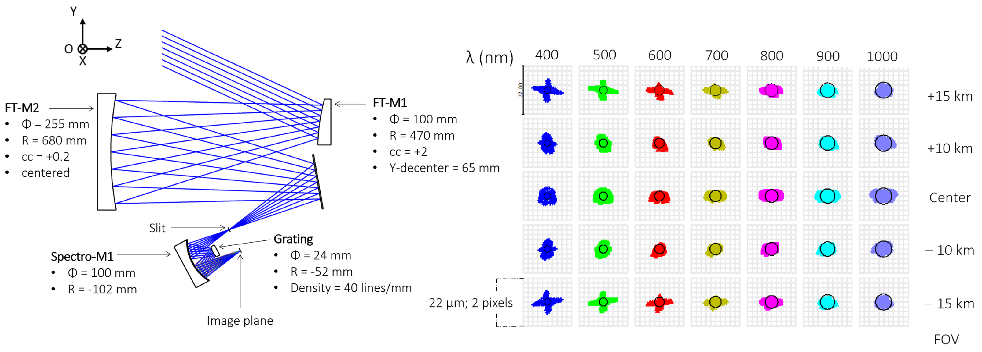
4.1. Optical Design and Theoretical Performance
4.2. Baffle Design, Windows, Filters and Coating Assumptions
5. Spatial and Spectral Responses and Contamination Level Comparing with Ghost Signal
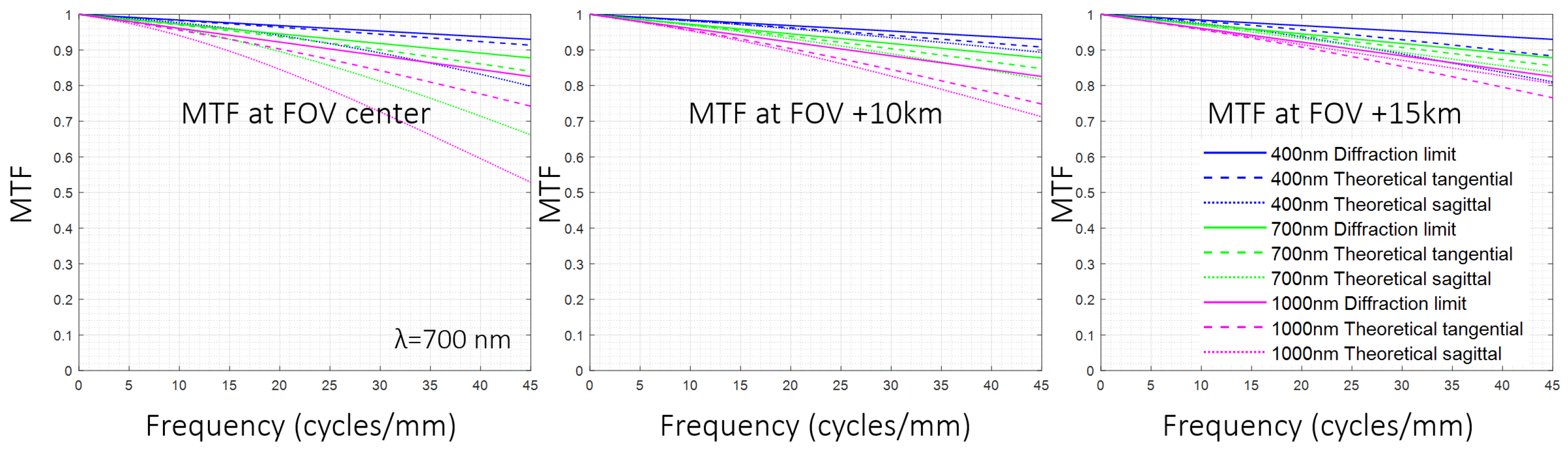
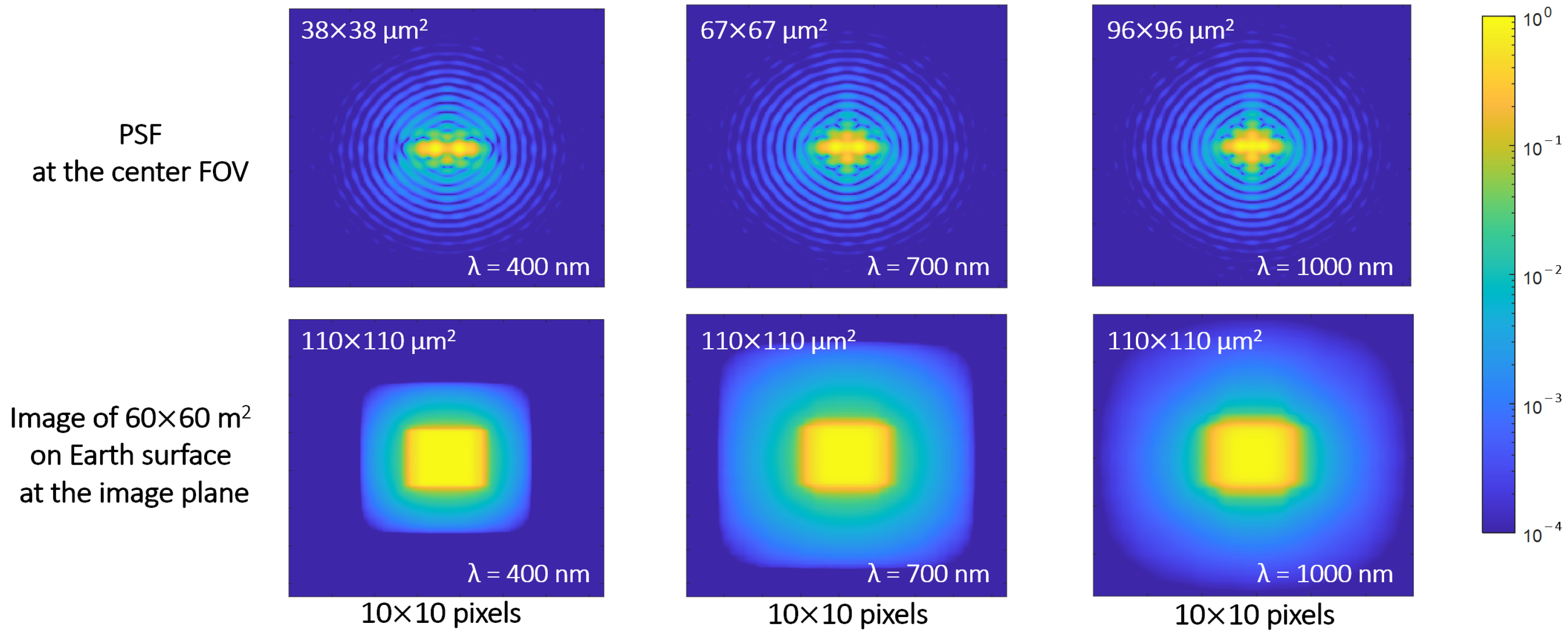
5.1. Instrument Response Considering the Aberrations and the Diffraction
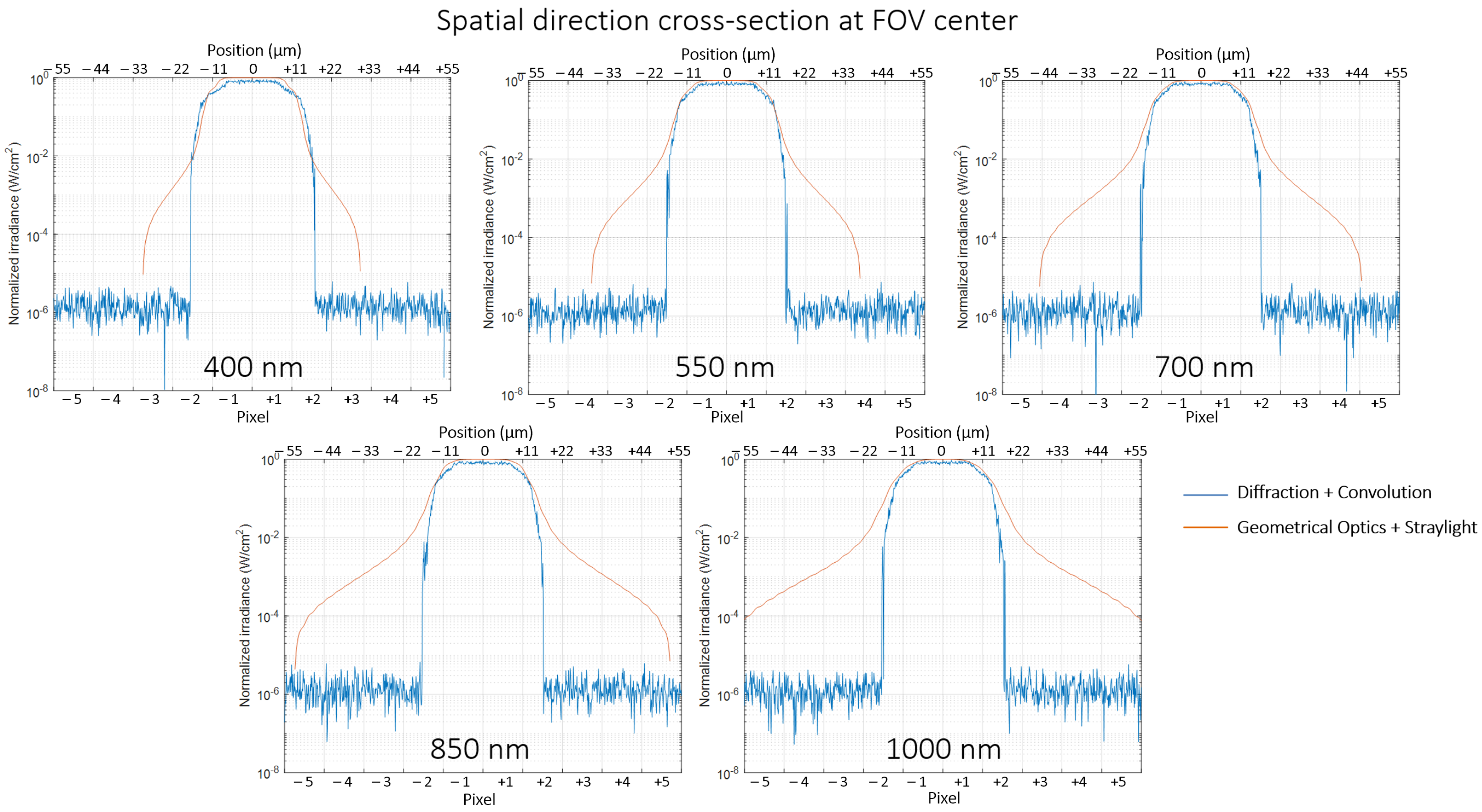
5.2. Straylight Background Irradiance
5.3. Contamination between Adjacent Pixels
6. Tolerancing and Performance Budget
6.1. Overall Method
6.2. Manufacturing Tolerancing Analysis
6.3. Assembly Tolerancing Analysis
6.4. Stability Tolerancing Analysis
6.5. Performance Budget
7. Radiometric Performances
7.1. Method and Assumptions
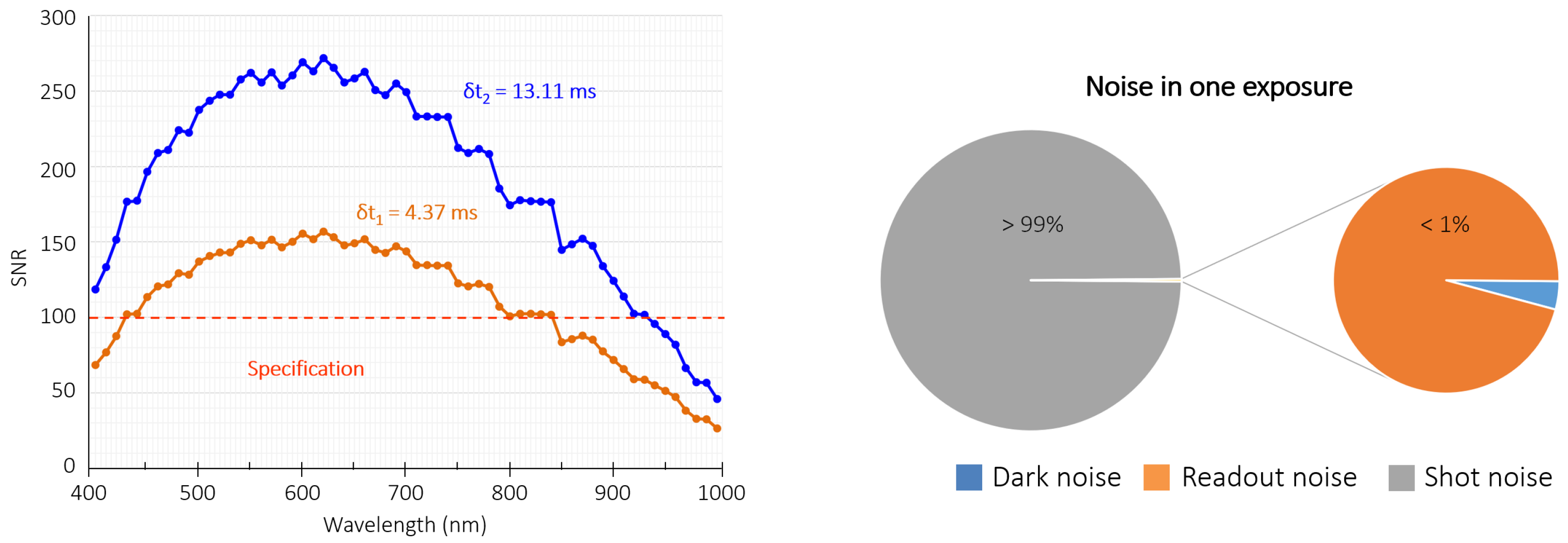
7.2. Results and Conclusions
8. Conclusions
Author Contributions
Funding
Acknowledgments
Conflicts of Interest
References
- Buisset, C.; Deboos, A.; Lepine, T.; Poshyachinda, S.; Soonthornthum, B. Design and performance estimate of a focal reducer for the 2.3 m Thai National Telescope. Opt. Express 2016, 24, 1416–1430. [Google Scholar] [CrossRef] [PubMed]
- Buisset, C.; Prasit, A.; Lepine, T.; Poshyachinda, S.; Soonthornthum, B.; Deboos, A. Opto-mechanical design and development status of an all spherical five lenses Focal Reducer for the 2.3 m Thai National Telescope. Proc. SPIE 2016, 9906, 99062F. [Google Scholar]
- Prasit, A.; Buisset, C.; Lepine, T.; Ridsdill-Smith, M.; Chakpor, A.; Leckngam, A.; Thummasorn, G.; Ngernsujja, S.; Inpan, A.; Kaewsamoet, P.; et al. Installation, alignment method, and preliminary test results of the Thai National Telescope focal reducer. Proc. SPIE 2019, 11116, 111161A. [Google Scholar]
- Lhospice, E.; Buisset, C.; Jones, H.R.; Martin, W.E.; Errmann, R.; Sithajan, S.; Boonsri, C.; Choochalerm, P.; Anglada-Escude, G.; Campbell, D.; et al. EXOhSPEC folded design optimization and performance estimation. Proc. SPIE 2019, 11117, 111170Z. [Google Scholar]
- Paenoi, J.; Buisset, C.; Suwansukho, K.; Sirichote, W.; Choochalerm, P.; Aukkaravittayapun, S.; Thummasorn, G.; Ngernsujja, S.; Inpun, A.; Kaewsamoeta, P.; et al. The Design and On-sky Results of the Prototype of a Low-Resolution Spectrograph for the Thai National Telescope. Curr. Appl. Sci. Technol. 2020, 20, 1. [Google Scholar]
- Drinkwater, N.R.; Rebhan, H. Sentinel-3: Mission Requirements Document, 2nd ed.; Mission Document; ESA: Paris, France, 2007. [Google Scholar]
- Sang, B.; Schubert, J.; Kaiser, S.; Mogulsky, V.; Neumann, C.; Forster, K.P.; Hofer, S.; Stuffler, T.; Kaufmann, H.; Muller, A.; et al. The EnMAP hyperspectral imaging spectrometer: Instrument concept, calibration, and technologies. Proc. SPIE 2008, 7086, 708605. [Google Scholar]
- Qian, S. Hyperspectral Satellites and System Design, 1st ed.; CRC Press: Boca Raton, FL, USA, 2020. [Google Scholar]
- Optical Design Software. Available online: https://www.zemax.com/pages/opticstudio (accessed on 1 August 2022).
- Wanajaroen, W.; Lepine, T.; Buisset, C.; Castelnau, M.; Costes, V.; Wannawichian, S.; Poshyachinda, S.; Soonthornthuma, B. Hyperspectral spectro-imager survey for state of art concept identification. Proc. SPIE 2021, 11852, 1185268. [Google Scholar]
- Gross, H. Handbook of Optical Systems Volume 4, 1st ed.; WILEY-VCH Verlag GmbH & Co. KGaA: Weinheim, Germany, 2008. [Google Scholar]
- Warren, D.W.; Gutierrez, D.J.; Hall, J.L.; Keim, E.R. Dyson spectrometers for infrared earth remote sensing. Proc. SPIE 2008, 7082, 70820R. [Google Scholar]
- Van Gorp, B.; Mouroulis, P.; Wilson, D.W.; Green, R.O. Design of the Compact Wide Swath Imaging Spectrometer (CWIS). Proc. SPIE 2014, 9222, 92220C. [Google Scholar]
- Van Gorp, B.; Mouroulis, P.; Wilson, D.W.; Green, R.O.; Rodriguez, J.I.; Liggett, E.; Thompson, D.R. Compact Wide swath Imaging Spectrometer (CWIS): Alignment and laboratory calibration. Proc. SPIE 2016, 9976, 997605. [Google Scholar]
- Reimers, J.; Bauer, A.; Thompson, K.P.; Rolland, J.P. Freeform spectrometer enabling increased compactness. Light Sci. Appl. 2017, 6, e17026. [Google Scholar] [CrossRef] [PubMed]
- Bass, M. Handbook of Optics: Fundamentals, Techniques, and Design, 2nd ed.; McGraw-Hill: New York, NY, USA, 1995. [Google Scholar]
- Acktar World Leader in Black Coating. Available online: https://www.acktar.com (accessed on 1 August 2022).
- Continuously Variable Filters (a.k.a. Linear Variable Filters)/CVSWP 395 nm–815 nm. Available online: https://www.deltaopticalthinfilm.com/product/cvswp-395-nm-815-nm (accessed on 1 August 2022).
- Manufacturing Tolerance Chart. Available online: https://www.optimaxsi.com/optical-manufacturing-tolerance-chart (accessed on 1 August 2022).
- AMS CMV-4000 CMOS Sensor Datasheet. Available online: https://ams.com/documents/20143/36005/CMV4000_DS000728_4-00.pdf (accessed on 1 August 2022).


| Parameter | Specification |
|---|---|
| Instrument concept | Visible Hyperspectral Imager |
| Orbit | Low Earth, Sun Synchronous Orbit |
| Altitude | 630 km |
| Spel domain | [400 nm, 1000 nm] |
| Ground Sampling Distance, FOV | 30 m, 30 km |
| Modulation Transfer Function | MTF > 0.3 at Nyquist Frequency |
| Spectral Response FWHM | 10 nm |
| Signal to Noise Ratio | SNR > 100 at L = 70 W/m/sr/m |
| Detector | CMOSIS CMV4000 |
| Pixel size and detector format | 11 m, 1000 × 120 |
| Mass | <30 kg |
| Dimension | <700 mm × 700 mm × 300 mm |
| Parameter | FT1 | FT2 | |
|---|---|---|---|
| M1 | Radius | 470 mm | 670 mm |
| Diameter | 100 mm | 100 mm | |
| Conic constant | +2 | +6.2 | |
| Off-axis decenter | 65 mm | 38 mm | |
| M2 | Radius | 680 mm | 640 mm |
| Diameter | 255 mm | 230 mm | |
| Conic constant | +0.2 | +0.2 | |
| Off-axis decenter | - | 105 mm | |
| Component | Parameter | Error | FT1 Max R (m RMS) | FT2 Max R (m RMS) |
|---|---|---|---|---|
| FT-M1 | Decenter X | ±0.1 mm | 1.8 | 0.9 |
| Decenter Y | ±0.1 mm | 2.2 | 2.3 | |
| Tilt X | ±0.1 degrees | 11.2 | 9.0 | |
| Tilt Y | ±0.1 degrees | 10.3 | 9.1 | |
| FT-M2 | Decenter X | ±0.1 mm | 1.8 | 0.9 |
| Decenter Y | ±0.1 mm | 2.6 | 2.3 | |
| Tilt X | ±0.05 degrees | 11 | 7.2 | |
| Tilt Y | ±0.05 degrees | 9.9 | 6.7 |
| System | Advantage | Drawback |
|---|---|---|
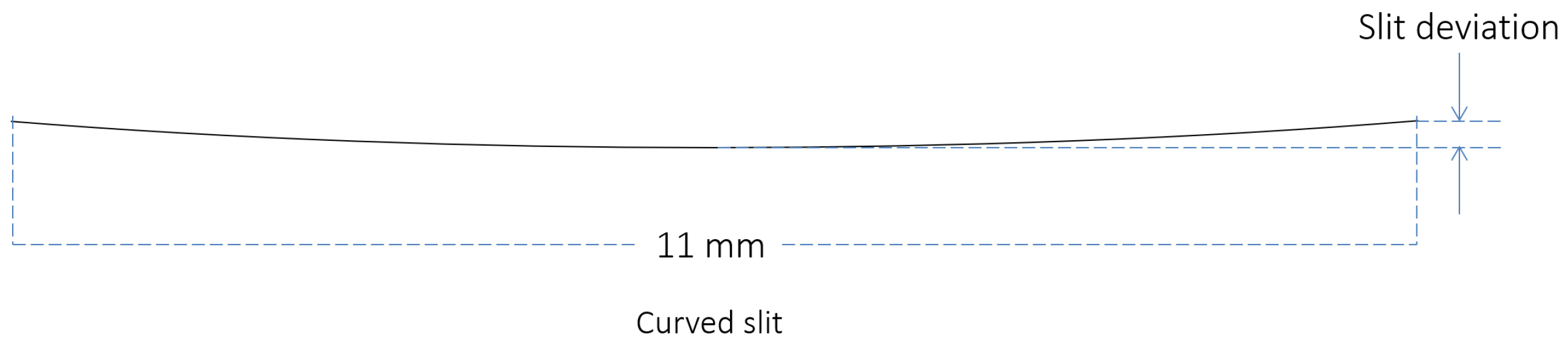
| FT1 | Physical and accessible Aperture Stop located on FT-M2 >Good control of straylight. One large centered concave mirror with a small deviation from reference sphere >Easy to manufacture and control. Only one small convex off-axis mirror with reasonable conic constant >Reasonable effort to manufacture and align. | Non-telecentric system >Not fully compatible with a telecentric spectrometer Smile distortion >Implies curved slit at spectrometer entrance |
| FT2 | Accessible Aperture Stop >Ease the baffling system design Telecentric system >Compatible with the telecentric spectrometer | Two off-axis aspherical mirrors and high conic constant for FT1- M1 >Difficult to manufacture and align, increase overall cost and risk. Higher volume than FT-1 to accommodate physical AS between M1 and M2 >Increases payload volume and mass. Smile distortion >Implies curved slit at spectrometer entrance |
| Component | Parameter | Error | Max R (m RMS) |
|---|---|---|---|
| Dyson lens | Decenter X | ±0.1 mm | 0.3 |
| Decenter Y | ±0.1 mm | 0.4 | |
| Tilt X | ±0.23 degrees | 0.8 | |
| Tilt Y | ±0.23 degrees | 0.3 | |
| Grating | Decenter X | ±0.1 mm | 0.3 |
| Decenter Y | ±0.1 mm | 0.6 | |
| Tilt X | ±0.17 degrees | 1.8 | |
| Tilt Y | ±0.17 degrees | 0.2 |
| Component | Parameter | Error | Max R (m RMS) |
|---|---|---|---|
| SP-M1 | Decenter X | ±0.1 mm | 0.2 |
| Decenter Y | ±0.1 mm | 1.1 | |
| Tilt X | ±0.1 degrees | 2.3 | |
| Tilt Y | ±0.1 degrees | 0.1 | |
| Grating | Decenter X | ±0.1 mm | 0.2 |
| Decenter Y | ±0.1 mm | 0.7 | |
| Tilt X | ±0.6 degrees | 3.7 | |
| Tilt Y | ±0.6 degrees | 0.7 |
| Design | Advantage | Drawback |
|---|---|---|
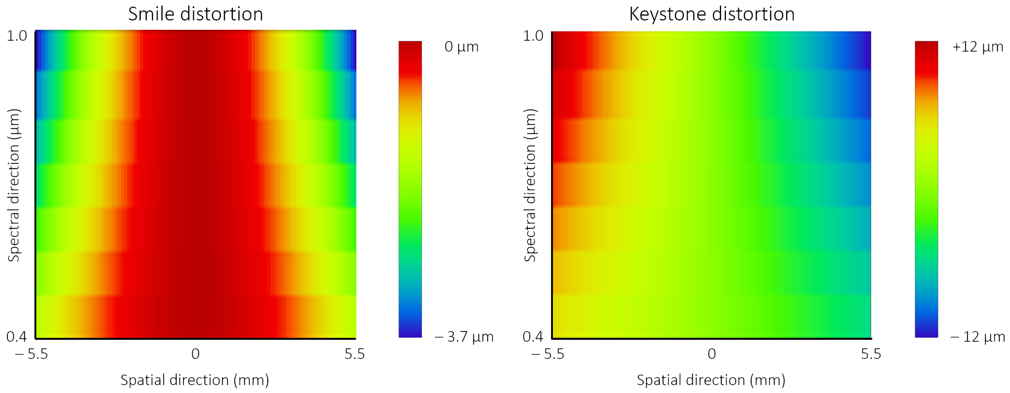
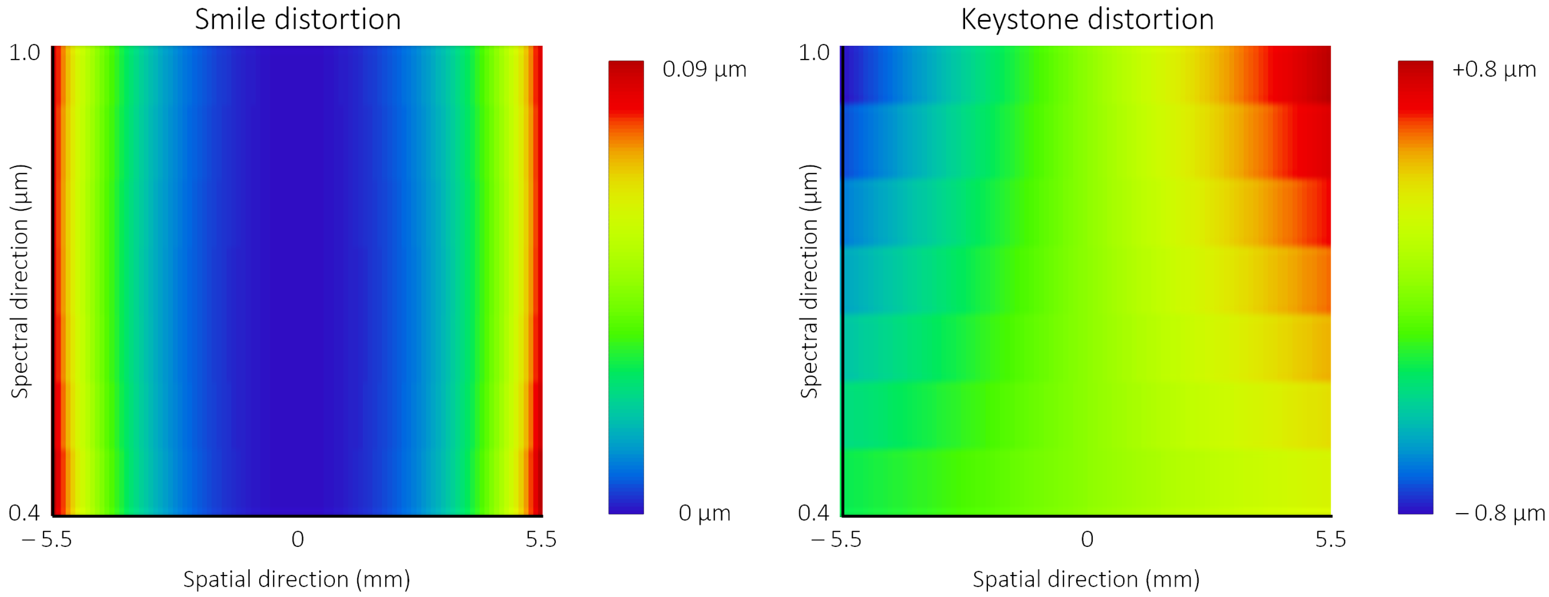
| Dyson Spectrometer | Simple optical elements >Easy to manufacture, cost-effective solution. Concave grating >Easy to manufacture and control. | Small volume available to accommodate filter, slit and detector >Increases AIT and AIV complexity and risk. High Keystone distortion Detector located close to Dyson lens >Increase the level of ghost image irradiance. |
| Offner Spectrometer | Better image quality and negligible distortion Design comprising one mirror and one grating only >Eases assembly and integration test and verification activities (AIT & AIV) | Convex blazed grating >Difficult and expensive to manufacture |
| Baffle Parameter | Value (mm) | |
|---|---|---|
| Entrance Baffle | 1st Vane External/Internal dimension | 140 × 120/110 × 78 |
| 2nd Vane External/Internal dimension | 140 × 120/109 × 78 | |
| 3rd Vane External/Internal dimension | 140 × 120/105 × 78 | |
| 4th Vane External/Internal dimension | 140 × 120/98 × 78 | |
| Distance between 1st vane–2nd vane | 70.3 | |
| Distance between 2nd vane–3rd vane | 75.4 | |
| Distance between 3rd vane–4th vane | 80.6 | |
| Telescope focal plane baffle | 1st Vane External/Internal dimension | 50 × 50/27.3 × 18 |
| 2nd Vane External/Internal dimension | 42.4 × 42.4/175.5 × 7 | |
| Distance between 1st vane–2nd vane | 30 | |
| Distance between 2nd vane—Slit | 20 | |
| Spot Radius Enlargement | Typical Case (68%) | Realistic Case (95%) | Worst Case |
|---|---|---|---|
| (m RMS) | 0.3 | 0.5 | 0.8 |
| (m RMS) | 0.5 | 1.0 | 1.8 |
| (m RMS) | 2.2 | 5.5 | 7.8 |
| (m RMS) | 2.3 | 5.5 | 8.0 |
| Spot Radius Enlargement | Typical Case (68%) | Realistic Case (95%) | Worst Case |
|---|---|---|---|
| (m RMS) | 1.5 | 1.5 | 1.5 |
| (m RMS) | 2.3 | 5.5 | 8.0 |
| (m RMS) | 3.8 | 7.1 | 9.5 |
| Parameter | Assumption |
|---|---|
| Dark and Readout noise | 125 e/s/pix @ 25 C and 13 e/pix |
| Pixel size | 11 m |
| Spectral radiance | 70 W/m2/sr/m |
| Spectral sampling, | 5 nm, 30 m |
| Flight altitude | 630 km |
| Optical payload throughput | T = 0.54 at = 700 nm |
| Aperture number | F/3 |
| Integration time | = 4.37 ms and = 13.11 ms |
| Attribute | Performance |
|---|---|
| - Selected FT RMS spot radius at FOV center | <2.2 m |
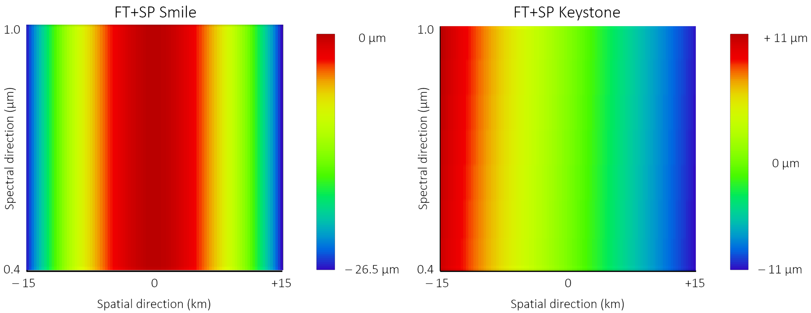
| - Selected FT distortions | Maximum 24 m at the edge of FOV |
| - Selected Spectrometer (Offner) RMS spot radius at = 700 nm and FOV center | 1 m |
| - Selected Spectrometer (Offner) distortions | Smile: <1 m |
| Keystone: <1 m | |
| - TSC-1 Hyperspectral Imager RMS spot radius at = 700 nm and FOV center | <1.5 m |
| - Theoretical system distortion | Maximum smile: 24.8 m @ the edge of FOV |
| Maximum keystone: <1 m | |
| - EOL spot radius at = 700 nm and FOV center | Typical: 3.8 m |
| Realistic: 7.1 m | |
| Worst: 9.5 m | |
| - Adjacent pixel contamination by diffraction at = 700 nm and FOV center | Spatial direction: 13% of the signal Spectral direction: 11% of the signal |
| - Adjacent pixel contamination by straylight at = 700 nm and FOV center | Spatial direction: 9% of the signal Spectral direction: 5% of the signal |
| - SNR > 150 for = 4.37 ms | [430 nm, 840 nm] |
| - SNR > 150 for = 13.11 ms | [400 nm, 910 nm] |
Publisher’s Note: MDPI stays neutral with regard to jurisdictional claims in published maps and institutional affiliations. |
© 2022 by the authors. Licensee MDPI, Basel, Switzerland. This article is an open access article distributed under the terms and conditions of the Creative Commons Attribution (CC BY) license (https://creativecommons.org/licenses/by/4.0/).
Share and Cite
Wanajaroen, W.; Buisset, C.; Lépine, T.; Chartsiriwattana, P.; Kosiyakul, M.; Prasit, A.; Saisutjarit, P.; Wannawichian, S.; Rujopakarn, W.; Poshyachinda, S.; et al. TSC-1 Optical Payload Hyperspectral Imager Preliminary Design and Performance Estimation. Photonics 2022, 9, 865. https://doi.org/10.3390/photonics9110865
Wanajaroen W, Buisset C, Lépine T, Chartsiriwattana P, Kosiyakul M, Prasit A, Saisutjarit P, Wannawichian S, Rujopakarn W, Poshyachinda S, et al. TSC-1 Optical Payload Hyperspectral Imager Preliminary Design and Performance Estimation. Photonics. 2022; 9(11):865. https://doi.org/10.3390/photonics9110865
Chicago/Turabian StyleWanajaroen, Weerapot, Christophe Buisset, Thierry Lépine, Pearachad Chartsiriwattana, Merisa Kosiyakul, Apirat Prasit, Phongsatorn Saisutjarit, Suwicha Wannawichian, Wiphu Rujopakarn, Saran Poshyachinda, and et al. 2022. "TSC-1 Optical Payload Hyperspectral Imager Preliminary Design and Performance Estimation" Photonics 9, no. 11: 865. https://doi.org/10.3390/photonics9110865
APA StyleWanajaroen, W., Buisset, C., Lépine, T., Chartsiriwattana, P., Kosiyakul, M., Prasit, A., Saisutjarit, P., Wannawichian, S., Rujopakarn, W., Poshyachinda, S., & Soonthornthum, B. (2022). TSC-1 Optical Payload Hyperspectral Imager Preliminary Design and Performance Estimation. Photonics, 9(11), 865. https://doi.org/10.3390/photonics9110865