Article

Volterra-Aided Neural Network Equalization for Channel Impairment Compensation in Visible Light Communication System

1
School of Electronic and Information Engineering, Qingdao University, Qingdao 266071, China
2
Normal College, Qingdao University, Qingdao 266071, China
3
Department of Electrical Engineering and Information Systems, The University of Tokyo, Tokyo 153-0041, Japan
*
Author to whom correspondence should be addressed.
Photonics 2022, 9(11), 845; https://doi.org/10.3390/photonics9110845
Submission received: 23 October 2022 / Revised: 2 November 2022 / Accepted: 7 November 2022 / Published: 10 November 2022
(This article belongs to the Special Issue Visible Light Communications)

Abstract

:
This paper addresses the channel impairment to enhance the system performance of visible light communication (VLC). Inspired by the model-solving procedure in the conventional equalizer, the channel impairment compensation is formulated as a spatial memory pattern prediction problem, then we propose efficient deep-learning (DL)-based nonlinear post-equalization, combining the Volterra-aided convolutional neural network (CNN) and long-short term memory (LSTM) neural network, to mitigate the system nonlinearity and then recover the original transmitted signal from the distorted one at the receiver end. The Volterra structure is employed to construct a spatial pattern that can be easily interpreted by the proposed scheme. Then, we take advantage of the CNN to extract the implicit feature of channel impairments and utilize the LSTM to predict the memory sequence. Results demonstrate that the proposed scheme can provide a fairly fast convergence during the training stage and can effectively mitigate the overall nonlinearity of the system at testing. Furthermore, it can recover the original signal accurately and exhibits an excellent bit error rate performance as compared with the conventional equalizer, demonstrating the prospect and validity of this methodology for channel impairment compensation.

1. Introduction

In order to tackle the explosive escalation of wireless data traffic and the emerging application services, the Sixth-Generation (6G) communication research is widely assumed to shift towards the higher-frequency spectrum since the current radio frequency (RF) band is becoming more and more crowded [1,2]. The millimeter-wave and terahertz spectrum can be widely developed to fulfill this demand; however, the corresponding equipment has an extremely high cost. Visible light communication (VLC) is expected to provide a potential supplement for 6G since it relies on the unlicensed spectrum spanning from 400 to 800 THz and has the benefits of electromagnetic interference resistance, green technology, safety, and low cost. In addition, VLC can be equipped with common lighting systems to allow simultaneous illumination and communication. During the last decade, various research works have been conducted to establish the theoretical foundation and application paradigm for high-speed VLC systems [3,4].
The spectral efficiency of VLC can be improved with the help of high-order modulation schemes [5,6]. Nevertheless, the special undesirable nonlinearities introduced by the electro-optical and photoelectric conversions will contaminate the useful signal [7], and the optical diffuse channel will also bring in an inevitable inter-symbol interference (ISI). The overall channel impairments should be relieved since they indeed significantly impair the signal performance and hinder the high-speed VLC transmission. Traditional schemes and algorithms can generally estimate the transfer function of the communication channel and remove the channel impairments by constructing nonlinear post-equalization (NPE) [7,8]. However, these methodologies still have a performance difference from the ideal case and would confront certain restrictions and requirements for different application scenarios.
The deep learning (DL) has shown great success in pattern identification, image recognition, and data mining. It has been already applied to physical layer communication due to its strong ability in learn the unknown or complex communication block [9,10], especially for modeling nonlinear phenomena. With the development of advanced network structures and optimized training algorithms, DL-based NPE shows unparalleled superiority compared to traditional approaches in channel impairment compensation. A comprehensive introduction and overview of DL-based methods can be found in [11,12,13,14,15,16,17,18,19,20,21,22,23,24,25]. In [12,13,14], the deep neural network (DNN) was employed to learn the channel characteristics and demodulate the output signals directly. In [15,16], the Gaussian-kernel-aided DNN networks were proposed as the pre-equalization and post-equalization, respectively, to mitigate the nonlinear degradation in high-order modulated VLC systems. In [17], a low-complexity memory-polynomial-aided neural network was created to replace the traditional post-equalization filters of carrierless amplitude and phase (CAP) modulation. These schemes utilizing the DNN can achieve the mitigation of the linear and nonlinear distortion of the VLC channel and exhibit better bit error rate (BER) performance than some existing methods. However, the learning ability of these DL models is limited in high-speed VLC since the system is mainly restricted by the inherent memory nonlinearity of the light-emitting diode (LED), resulting in a slow convergence speed and relatively poor generalization of the DNN.
For a nonlinear VLC channel with memory, the recurrent neural network (RNN) with long short-term memory (LSTM) cells seems to be a better choice for memory sequence prediction, because the long-term memory parameters can store the channel characteristics. In [18], a memory-controlled LSTM equalizer was proposed to compensate both the linear and nonlinear distortions. In [19], an LSTM network was proposed to handle with the nonlinear distortions for a pulse amplitude modulation (PAM) system with the intensity modulation and direct detection (IM/DD) link over 100 km standard single-mode fiber. These proposed LSTM models outperform the conventional model-solving-based equalizers; nevertheless, the output equalization accuracy does not possess a good robustness to the noise variation, leading to the degradation of learning efficiency. In order to learn more suitable channel features, the convolutional neural network (CNN) can be used for memory sequence prediction from raw channel outputs [20], since a function could be learned that maps a sequence of past observations as the input to an output observation. In [21], an equalization scheme using the CNN was proposed in an orthogonal-frequency-division-multiplexing (OFDM)-based VLC system for direct equalization. In [22], a novel blind algorithm based on the CNN was introduced to jointly perform equalization and soft demapping for M-ary quadrature amplitude modulation (M-QAM). The results showed that the proposed CNN schemes outperform the existing equalization algorithms and can maintain an excellent BER performance in the linear and nonlinear channel. However, for dynamic and deep memory scenarios, it obtains the optimal equalization performance at the cost of computational complexity, because the dimension of the input spatial information increases sharply and the convolution layer has to undertake tremendous computational pressure, resulting in the increase of network complexity [23]. In order to shrink the network complexity, a specific architecture combination was proposed to distribute the learning task [24,25]. However, the original input data hardly experienced effective transformation, resulting in a large amount of time cost in the training process to extract the implicit features contained in the samples. Hence, the trade-off among computational complexity, training times, robustness, and generalization is one of the critical challenges and should be further developed in practical VLC applications. Besides, it is also necessary to consider how to consolidate the virgin data into alternate forms by changing the value, structure, or format so that the data may be easily parsed by the machine.
In this paper, inspired by the approaches in [15,16,17,18,19,20,21,22,23,24,25], the channel impairment compensation is formulated as a spatial memory pattern prediction problem, and an efficient impairment compensation scheme in terms of a model-driven-based CNN-LSTM is proposed to undo the memory nonlinearity of VLC. The underlying idea is that the Volterra structure is applied to pre-emphasize the original sequence and the appropriate pattern is formed as the spatial input accordingly. Then, a hybrid CNN and LSTM neural network is elaborately designed to learn the implicit feature of nonlinearity and predict the memory sequence directly, which can speed up the convergence process and improve the equalization accuracy. The main contribution of this work can be summarized as follows:
  • The structure information of the Volterra model is involved in the proposed DL equalizer to pre-emphasize the virgin data, which is favorable for the memory feature learning. Therefore, it can relax the learning pressure and reduce the structural complexity and training time.
  • Based on the traditional model-solving procedure, the channel impairment compensation is formulated as a spatial memory pattern prediction problem, and the proposed DL model is ingeniously used to achieve the accurate prediction.
  • Both the memory nonlinearity of the LED and the dispersive effect of the optical channel in a VLC system are simultaneously considered during the training stage.
  • The proposed scheme can still provide an excellent BER performance under the mismatched conditions of training and testing, showing a good robustness.
Numerical simulations in terms of the learning and generalization show that the proposed scheme is able to predict the original transmitted signal and compensate the impairments with high accuracy and resolution. In addition, it can converge relatively fast to achieve a better normalized-mean-squared error (NMSE), which confirms its superiority to some existing methods.
The remainder of this paper is organized as follows. In Section 2, the overall channel nonlinearity is analyzed and the impairment compensation is formulated as a spatial memory pattern prediction problem. The corresponding network architecture and training specification are illustrated in Section 3. Simulation results and discussions are demonstrated in Section 4, and conclusions are given in Section 5.
Notations: Matrices and column vectors are denoted by upper and lower boldface letters, respectively. x n denotes the n-th element of x . The set of real numbers is denoted by R . In addition, *, ⊗, · T , and | · | are employed to represent the convolution, the Kronecker product, the transpose, and the absolute operators, respectively. Let · p denote the p -norm and a ˜ be an estimation of the parameter of interest a. N μ , σ 2 is the Gaussian distribution with mean μ and variance σ 2 .

2. System Nonlinearity

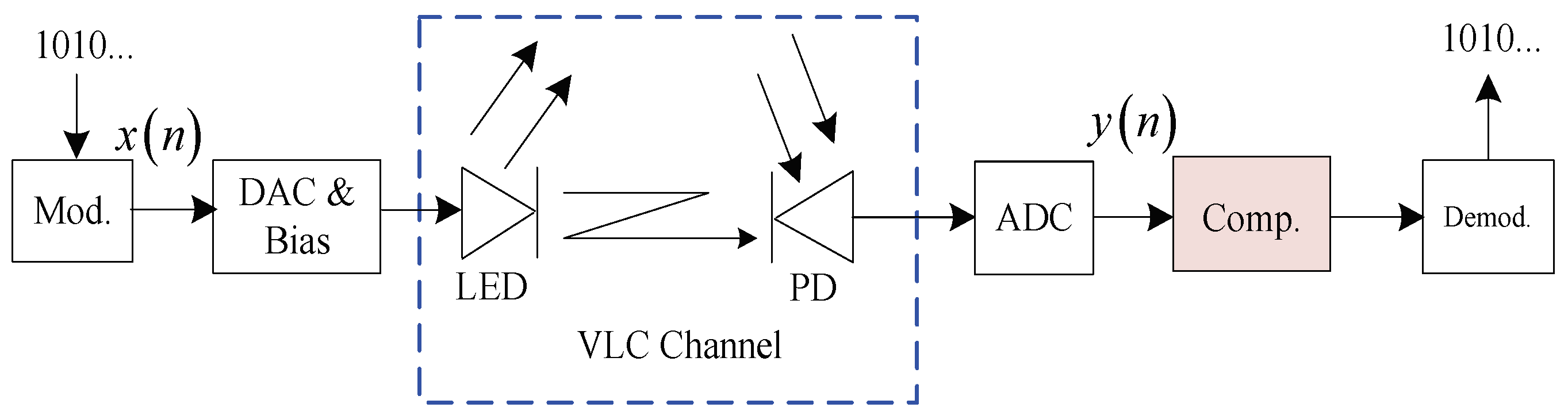
A typical VLC system employing an IM/DD structure is illustrated in Figure 1. The end-to-end VLC channel includes an electrical modulator, digital-to-analog converter (DAC), bias tee, LED, optical transmission channel, analog-to-digital converter (ADC), and electrical demodulator. Numerous modules will generate nonlinearities. However, the overall nonlinearity of the VLC channel is mainly introduced by both the LED and multipath propagation of the optical link. In addition, the memory nonlinearity is more significant as the signal bandwidth is increased. The LED behaviors are usually described by the Wiener model, which is a cascade of linear and nonlinear blocks. Let f 0 denote the 3 dB cut-off frequency, then the memory nonlinearity of the LED can be expressed as
h 1 n = exp 2 π n f 0 .
The memoryless nonlinearity block can be modeled by
f 1 x n = q = 0 Q a q x q n ,
where x n is input real-valued transmitting signal, a q is the coefficient, and Q is the polynomial order. The channel impulse response (CIR) of the multipath propagation effect in VLC can be expressed by the following:
h 2 n = i = 1 N r P i δ n τ i ,
where P i is the optical power, τ i is the propagation time of the i-th light ray, and N r is the number of received rays at the photodetector (PD), respectively. In fact, the PD also exhibits nonlinear behavior as the optical intensity of the injected signal is very large, leading to the saturation of the PD. However, the optical intensity can be lowered with the help of an optical attenuator. Therefore, the PD can be regarded as a linear component, which is always modeled by the Dirac function. Note that the quantification effect in the ADC is not considered here. After optical-to-electrical conversion in the PD, the received electrical signal can be expressed as
y n = R P D f 1 x n + I D C * h 1 n * h 2 n + ε n ,
where R P D denotes the responsivity of the PD, I D C is the DC bias, and ε n is the Gaussian noise following N 0 , σ ε 2 .
At the receiver, y n is fed into the Volterra-based NPE. Then, the corresponding outputs can be expressed as
x ˜ n = h 0 + k 1 = 0 L 1 h 1 k 1 y n k 1 + k 1 = 0 L 1 k 2 = 0 L 1 h 2 k 1 , k 2 i = 1 2 y n k i + + k 1 = 0 L 1 k P = 0 L 1 h P k 1 , , k P i = 1 P y n k i + v n = p = 0 P k 1 = 0 L 1 k p = 0 L 1 h p k 1 , , k p i = 1 p y n k i + v n ,
where L denotes the memory length, P is the nonlinear order, h p k 1 , , k p is the p-th order of the Volterra kernels, and v n is the modeling error. Let
y 1 n = y n , , y n L + 1 T ,
represent the truncated samples with length L, which contains both the current and the past channel outputs.
As seen from (5), the calculation of x ˜ n is mainly related to y 1 n and h p k 1 , , k p . As we known, the main goal of the NPE is to produce the desired x ˜ n from y 1 n to minimize the error with respect to x n , which indicates that the useful information of x ˜ n is involved in y 1 n . In other words, we can infer that x ˜ n can be predicted from y 1 n once all the h p k 1 , , k p are well obtained. Therefore, from the perspective of learning and classification, both the h p k 1 , , k p and x ˜ n can be learned from the training sample set x n , y 1 n , and the implement of the NPE can be formulated as a prediction problem, where the DL approach is very appropriate.

3. The Proposed Scheme

As we know, LSTM is more powerful in dealing with the memory sequences’ prediction problem since it could handle the long-term dependencies and store the memory parameters, which are related to the channel characteristics. As regards the VLC system, y n experiences the complex optical-to-electrical and electrical-to-optical conversion, and the complicated overall channel nonlinearity involved in y n is very implicit and not very intuitive, which will greatly increase the computational complexity and learning difficulty. Furthermore, it leads to a slow convergence speed and the decrease of equalization performance. In order to improve the learning ability and accelerate the convergence speed, we therefore propose a novel impairment compensation scheme, which utilizes the Volterra structure to construct the spatial features and feed them into the CNN-LSTM network to extract the characteristic of memory nonlinearity. In the following analysis, we assume that the system synchronization has been already achieved at the receiver.

3.1. Input Preprocessing Based on Volterra Feature

The composition and structure of the virgin input data can directly affect the performance of deep learning. Due to the complexity of the VLC channel, it is very necessary to transform or encode y n so that it may be easily parsed by the machine. The main agenda for the proposed model to be accurate and precise in its predictions is that the algorithm should be able to easily interpret the data’s features. As demonstrated in (5), for p 2 , x ˜ n can be considered as the sum of the response for each h p k 1 , , k p and y p ( n ) , shown as
x ˜ n = p = 0 P y p T n h p + v n ,
where y p n = y p 1 n y 1 n , and h p denotes the corresponding kernel coefficients for h p k 1 , , k p . Let y n = 1 , y 1 T n , , y P T n T . (7) can be further formed as
x ˜ n = y T n h + v n ,
where h = h 0 T , h 1 T , , h P T T is the Volterra kernel vector and h p contains the corresponding kernel coefficients h p k 1 , , k p , which are arranged sequentially for the index k 1 , , k p .
Therefore, y n should be firstly stacked for the last L points shown in (6) and then transformed into the sequence y n by using the above approach based on the Volterra structure feature. In order to shrink the computational complexity and speed up the learning progress, the sequence y n is truncated with a 2 m length. Then, the first appropriate pattern can be formed by the following way, shown as
Y 1 = y 1 y 2 y m y 2 y 3 y m + 1 y m y m + 1 y 2 m 1 .
With the time sliding window moving forward one step, the second pattern can be generated by
Y 2 = y 2 y 3 y m + 1 y 3 y 4 y m + 2 y m + 1 y m + 2 y 2 m .
Until the last N-th points, multiple patterns Y ¯ can be obtained subsequently, which will enter the neural network as the features for the input layer. Note that the step of the sliding window was set as 1 in this paper, and m also denotes the time step used in the following DL model.

3.2. Network Structure

The architecture of the proposed model is depicted in Figure 2, which is composed by subnet S 1 with L 1 convolution layers, subnet S 2 with L 2 LSTM layers, and subnet S 3 with L 3 dense layers.
The samples Y ¯ R N 2 m + 2 × m × m are then fed into S 1 for feature extraction. The structure of S 1 is composed of a convolution layer, pooling layer, flatten layer, and dense layer. The convolution layer employs a series of two-dimensional convolution filters (2D-Conv) to Y ¯ , so as to extract different feature maps of received signals. Let K l and C l denote the size of the convolutional kernel and the number of filters of the l-th convolutional layer, respectively. For simplicity, the stride was fixed to 1, and the Relu function and the same padding were employed in 2D-Conv. After the convolution calculation, the max-pooling layer is used to extract the invariant features with the non-linear downsampling, which will eliminate the non-maximal values. The same signal processing is implemented in the next 2D-Conv and max-pooling layer. After that, the flatten layer is employed to reshape the data size, and then, the dense layer is linked behind accordingly.
The CNN outputs should be firstly transformed as a three-dimensional vector Y ¯ 1 R N 2 m + 2 × m × D 1 S 2 and fed into S 2 , where D 1 S 2 denotes the cell number of the first layer of S 2 . The structure of S 2 is made up by cascaded sub-layer blocks composed by multiple LSTM cells. In addition, different amounts of LSTM cells can be deployed in different sub-layers. The internal structure of a single LSTM cell, as shown in Figure 2, contains three Sigmoid gates in terms of the forget gate, input gate, and output gate. These gates can selectively influence the model state at each time step. The forget gate is also the core of a single LSTM cell, since it determines the information that should be retained or discarded according to the current input y t and the previous output H t 1 . The output of forget gate can be expressed as
f t = σ W f · y t , H t 1 + b f ,
where σ is the Sigmoid function and W f and b f represent the parameter matrix and bias matrix of the forget gate, respectively. After forgetting part of the previous state, the input gate picks up some new information and then adds it into the former state C t 1 . Therefore, the new cell state is formed as
C t = f t C t 1 + i t z t ,
where z t denotes the temporary cell state and i t is the output of the input gate. Furthermore, the expression of z t is given as
z t = tanh W z · y t , H t 1 + b z ,
and the output i t can be expressed as
i t = σ W i · y t , H t 1 + b i ,
where W z , W i , b z , and b i denote the parameter matrix and bias matrix, respectively. Therefore, the value f t and i t between 0 and 1 also indicates the proportion of the important information in C t 1 and z t , thereby determining which information is to be updated. Then, the output of the LSTM cell can be calculated by
H t = tanh C t σ W o · y t , H t 1 + b o .
As a result, the outputs of this layer are fed into the corresponding LSTM cell of the next layer. However, as for the last layer, only the H m at the last time step is selected and then composed as the final output H L R N 2 m + 2 × D L 2 S 2 , where D L 2 S 2 denotes the cell number of the last layer in S 2 . In this case, H L should be transformed as a column vector to be fed into the dense net S 3 to refine the output results. Note that the linear activation function is deployed in S 3 without normalization. Finally, the equalized x ˜ R 2 N 2 m + 2 can be directly obtained at the output of S 3 , and the overall VLC nonlinearity will be efficiently compensated by using the proposed scheme.

3.3. Complexity

For the computational complexity, it is worth noting that the calculation of S 1 and S 2 is dominant in each time step. Let M l be the spatial size of the output feature map in the l-th convolutional layer, which can be calculate by
M l = I l K l + 2 P l + 1 ,
where I l is the input matrix size and P l is the padding length. Furthermore, we define the cell number of each layer in S 2 as equal to D l S 2 . Accordingly, the overall complexity of the proposed model per time step can be approximately expressed as
Ξ O l = 1 L 1 K l 2 C l C l 1 + M l 2 C l + l = 1 L 2 4 m D l S 2 + 4 D l S 2 2 .

3.4. Training Strategy

The proposed scheme was trained by viewing the VLC channel as a black box. Fortunately, researchers have developed several reference channel models for indoor environments for VLC [26]. Therefore, the training data can be easily obtained by simulations [12]. As for collecting the training set, the receiving plane is divided into several grid units with equidistant spacing used as potential locations for the PD. After VLC transmission and optical-to-electrical conversion, the received signals are collected under different PD locations. With the skillful preprocessing of the received signal, every spatial pattern and one sample of the transmitted signals are combined as the training data. Practically, we should collect a diverse and abundant training set, including the potential PD locations, to enhance the parameters learning ability of the proposed scheme.
The direct-current-biased optical (DCO)-OFDM, containing in total 512 sub-carriers with 16-QAM constellation mapping, is adopted as the training symbol, and only five symbols are randomly generated in each training epoch. Moreover, the NMSE between the raw x and the equalized x ˜ is employed as the training loss function, demonstrated by
l o s s = x x ˜ 2 2 x 2 2 .
Note that the DC gain is removed from the training set so that the training loss of the proposed scheme can be fairly evaluated. Furthermore, the training procedure was implemented using TensorFlow on a work station running with a graphics processing unit (GPU) of NVIDIA GeForce 2080Ti; the adaptive moment estimation (Adam) was adopted as the optimizer, and the learning rate was fixed to 0.0001. As in the testing stage, only several special links were adopted to evaluate the system performance for the simplicity of the demonstration.

4. Simulation Results

Simulations were conducted to evaluate the performance of the proposed scheme for channel nonlinearity compensation. The parameter of the IM/DD channel follows the case shown in [7]. As for the network architecture, the convolution block in S 1 employs only one convolution layer and one pooling layer, in which both the pooling size and stride step were set as 2. The S 2 involves two LSTM layer with the cell size of ( 128 , 256 ) . The S 3 employs one dense layer with the neuron size of 50. It is noteworthy that the amount of filters, in terms of C l in S 1 , should be set equal to the time step m in S 2 based on empirical trials. In addition, the testing set should be chosen different from that for training.

4.1. Convergence Performance

As the time step m was fixed to 40 and the kernel size K was three, the training cost of the proposed scheme is demonstrated in Figure 3, where the training signal-to-noise ratio (SNR) λ varies from 30 to 60 dB . As the results show, the loss curves with different λ tend to be stable gradually as the training epoch increases. The average final loss of the proposed scheme for λ = 40 , 50 and 60 dB is around 26.5 dB . In addition, it can be seen from the figure that the proposed scheme trained under the samples with a large λ converges faster than the one for a small λ , e.g., the case with λ = 40 dB costs about 2500 epochs to achieve convergence, whereas it would use 1800 epochs for the one of λ = 50 dB . In general, the quality of training samples indeed affects the learning ability of a customized DL model to a certain extent; however, it is not dominant in the training process.
As the time step m was fixed to 30 and the kernel size K varied from 2 to 5, the corresponding NMSE loss is presented in Figure 4. All of the curves tend to be stable gradually with the training epoch increased and eventually achieve an acceptable training performance, e.g., the final loss for K = 5 remains around 27.5 dB , and that for K = 4 is 28.2 dB , which indicates successful network training since they are favorable for a QAM symbol recovery. We can also observe that the kernel size indeed had a significant effect on the convergence performance. In fact, as K increased, the larger the receptive field obtained during the training, resulting in the extracted features being more global and discriminative. However, this will bring about a sharp increase in the amount of parameter calculation. Nevertheless, the small value of K will lead to insufficient feature learning, which is unfavorable for network convergence. However, the model trained under K = 4 converged faster and only cost about 1700 epochs to achieve an NMSE of less than 27 dB .
Figure 5 shows the training performance for different time steps. The average final loss of the last 1000 epochs was 24.18 , 26.18 , 28.58 , and 30.58 dB for m = 10 , 20, 30, and 40, respectively. The figure indicates that the larger the m used, the smaller the training NMSE achieved is. However, as m is set too large, the size of the input spatial pattern will increase, which will not only increase the complexity in the convolution operation, but also increase the difficulty in LSTM prediction. Moreover, the network structure will become intricate. Under the consideration of convergence speed and training quality, m = 30 , K = 4 was employed in the following model, although the kernel size was an even value.

4.2. Nonlinearity Compensation

The time domain amplitude outputs of the proposed scheme and the original received y n are illustrated in Figure 6. For a fair comparison, the amplitude outputs of the ideal equalization case are also depicted here, where the channel information is perfectly known to the receiver. From the figure, it can be observed that the amplitudes of the original received y n are severely distorted as compared with the ideal case. However, with the help of an effective feature learning, the proposed scheme can exactly predict a similar amplitude output as the ideal case.
The corresponding power spectral density (PSD) performance comparison is demonstrated in Figure 7. As shown in the figure, the overall nonlinearity of the IM/DD channel is manifested in the manner of in-band distortion and out-band spectral regrowth. However, the PSD of the proposed scheme shows a similar curve as compared with that of the ideal case. Although the sideband level at a high frequency is slightly inconsistent with that of the ideal case, it does not affect the signal demodulation because the power of useful information is mainly located at the in-band PSD. Therefore, the detrimental distortions can be well compensated by the proposed DL model.
The corresponding BER performance is illustrated in Figure 8 as the testing SNR ζ varied from 0 to 36 dB . In addition, the other three schemes in terms of the DNN [13], the LSTM [19], and the CNN compensator [21] are also presented here. In general, the proposed scheme has the closest BER performance to the one for the ideal case, and the BER accuracy of the DNN scheme tends to be saturated when ζ is over 27 dB . As for the same BER of 1 × 10 3 , the proposed scheme can reduce the required SNR at least by 2.5 dB as compared with the LSTM approach and nearly by 14.2 dB as compared with the DNN method, which shows the superiority of the proposed scheme for nonlinearity mitigation. The channel characteristics can be perfectly revealed and then learned by the proposed scheme, and it can still work effectively even though the testing conditions are not exactly the same as the channel noise used in the training stage, which shows the good generalization ability of the proposed model. Besides, the CNN scheme can also provide an excellent BER performance as compared with the DNN and LSTM methods, because the CNN offers dilated convolutions, in which the convolution layer could handle the spatial information and store the memory. However, there will be more computation time in the training phase to achieve the convergence, which is analyzed next.

4.3. Complexity

The corresponding application complexity in terms of the amount of floating-point operations (FLOPs), convergence cost, and average training time consumption in each epoch is shown in Table 1. Notice that the FLOPs were measured based on the frozen graph and different platforms may cost different training times. In addition, the corresponding complexity of the DNN scheme is not demonstrated because it converges at an unacceptable training accuracy. As the results show, although the LSTM costs less FLOPs, the learning ability is limited since it achieves the worst accuracy as compared with the other two schemes. The CNN converges with relatively more epochs and costs much training time, because all input features must be analyzed by the convolution procedure and the corresponding input features are directly obtained from the original received signal without any transformation. Under memory nonlinearity scenarios, the CNN has higher structural complexity and introduces more convolution and pooling layers to achieve the equivalent target accuracy as that of the proposed scheme. By comparison, since the special customized input patterns based on the Volterra model were employed, the proposed scheme exhibits better learning efficiency and only requires 1750 epochs to achieve convergence. Moreover, it only needs 755.6 million FLOPs to achieve the equivalent BER performance, nearly one-third of the CNN. Note that the amount of FLOPs is also related to the number of input signals. Therefore, the proposed Volterra-aided DL scheme can effectively balance the performance and application complexity as compared with the original CNN scheme.

4.4. Robustness Analysis

The well-trained model was valuated at different receiver locations. For convenience, the four PD locations with the root mean square (RMS) delay spread of 7.92, 8.2, 8.3, and 8.9 ns, marked as U 1 , U 2 , U 3 , and U 4 , were employed in the testing, respectively. The corresponding results are shown in Figure 9. As clearly seen from the figure, the BER performances of these four cases are very similar under the low-SNR region and only have a slight difference for a high SNR. Therefore, the proposed model can still work effectively and can provide robust BER performance even though the testing conditions are not exactly the same as those used in the training stage, showing a good robustness and generalization ability of the proposed scheme.

5. Conclusions

In this paper, we proposed a Volterra-aided DL equalizer for the channel impairment compensation in a VLC system. Benefiting from the customized spatial pattern and the elaborate cascaded network structure, the proposed scheme exhibits unique advantages in channel characteristics’ learning. In addition, it can speed up the convergence process and improve the equalization accuracy. The results show that the proposed scheme is favorable to mitigate the overall nonlinearity of the VLC channel and can achieve an excellent BER performance improvement, which significantly outperforms the conventional DL-based equalizers compared at the same BER level. Moreover, it shows robustness to the mismatch conditions of the practical deployment and training stages.

Author Contributions

Conceptualization, P.M. and W.Y.; methodology, P.M. and H.P.; software, D.T. and W.Y.; validation, D.T. and X.L.; formal analysis, P.M. and H.P.; data curation, D.T. and X.L.; writing—original draft preparation, P.M., D.T. and H.P.; writing—review and editing, P.M. and H.P.; visualization, D.T. and H.P.; grammar check, H.P.; supervision, P.M. and H.P.; funding acquisition, P.M. All authors have read and agreed to the published version of the manuscript.

Funding

This research was partially funded by the Shandong Provincial Natural Science Foundation under Grant ZR2019BF001, by the National Natural Science Foundation of China (NSFC) under Grant 61801257, by the China Postdoctoral Science Foundation under Grant 2019M652322, and by the China Scholarship Council. The APC was funded by Shandong Provincial Natural Science Foundation under Grant ZR2019BF001.

Institutional Review Board Statement

Not applicable.

Informed Consent Statement

Not applicable.

Data Availability Statement

The data presented in this study are available upon reasonable request.

Acknowledgments

The authors express their gratitude to the Editors and the anonymous Reviewers for their insightful suggestions and general assistance.

Conflicts of Interest

The authors declare no conflict of interest.

References

  1. You, X.; Wang, C.X.; Huang, J.; Gao, X.; Zhang, Z.; Wang, M.; Huang, Y.; Zhang, C.; Jiang, Y.; Wang, J.; et al. Towards 6G wireless communication networks: Vision, enabling technologies, and new paradigm shifts. Sci. China Inf. Sci. 2021, 64, 110301. [Google Scholar] [CrossRef]
  2. Letaief, K.B.; Chen, W.; Shi, Y.; Zhang, J.; Zhang, Y.J.A. The Roadmap to 6G: AI Empowered Wireless Networks. IEEE Commun. Mag. 2019, 57, 84–90. [Google Scholar] [CrossRef] [Green Version]
  3. Li, X.; Zhang, R.; Hanzo, L. Optimization of Visible-Light Optical Wireless Systems: Network-Centric Versus User-Centric Designs. IEEE Commun. Surv. Tutor. 2018, 20, 1878–1904. [Google Scholar] [CrossRef] [Green Version]
  4. Linnartz, J.P.M.G.; Deng, X.; Alexeev, A.; Mardanikorani, S. Wireless Communication over an LED Channel. IEEE Commun. Mag. 2020, 58, 77–82. [Google Scholar] [CrossRef]
  5. Jia, L.; Shu, F.; Huang, N.; Chen, M.; Wang, J. Capacity and Optimum Signal Constellations for VLC Systems. IEEE OSA J. Light. Technol. 2020, 38, 2180–2189. [Google Scholar] [CrossRef] [Green Version]
  6. Zhang, S.; Wei, Z.; Cao, Z.; Ma, K.; Chen, C.J.; Wu, M.C.; Dong, Y.; Fu, H.Y. A High-Speed Visible Light Communication System Using Pairs of Micro-size LEDs. IEEE Photonics Technol. Lett. 2021, 33, 1026–1029. [Google Scholar] [CrossRef]
  7. Miao, P.; Chen, G.; Wang, X.; Yao, Y.; Chambers, J. Adaptive Nonlinear Equalization Combining Sparse Bayesian Learning and Kalman Filtering for Visible Light Communications. IEEE OSA J. Light. Technol. 2020, 38, 6732–6745. [Google Scholar] [CrossRef]
  8. Mitra, R.; Bhatia, V.; Jain, S.; Choi, K. Performance Analysis of Random Fourier Features-Based Unsupervised Multistage-Clustering for VLC. IEEE Commun. Lett. 2021, 25, 2659–2663. [Google Scholar] [CrossRef]
  9. Wang, T.; Wen, C.K.; Wang, H.; Gao, F.; Jiang, T.; Jin, S. Deep learning for wireless physical layer: Opportunities and challenges. China Commun. 2017, 14, 92–111. [Google Scholar] [CrossRef]
  10. Huang, H.; Guo, S.; Gui, G.; Yang, Z.; Zhang, J.; Sari, H.; Adachi, F. Deep Learning for Physical-Layer 5G Wireless Techniques: Opportunities, Challenges and Solutions. IEEE Wirel. Commun. 2020, 27, 214–222. [Google Scholar] [CrossRef]
  11. Shi, J.; Niu, W.; Ha, Y.; Xu, Z.; Li, Z.; Yu, S.; Chi, N. AI-Enabled Intelligent Visible Light Communications: Challenges, Progress, and Future. Photonics 2022, 9, 529. [Google Scholar] [CrossRef]
  12. Miao, P.; Yin, W.; Peng, H.; Yao, Y. Study of the performance of deep learning-based channel equalization for indoor visible light communication systems. Photonics 2021, 8, 453. [Google Scholar] [CrossRef]
  13. Ye, H.; Li, G.Y.; Juang, B. Power of Deep Learning for Channel Estimation and Signal Detection in OFDM Systems. IEEE Wirel. Commun. Lett. 2017, 7, 114–117. [Google Scholar] [CrossRef]
  14. Gao, X.; Jin, S.; Wen, C.K.; Li, G.Y. ComNet: Combination of Deep Learning and Expert Knowledge in OFDM Receivers. IEEE Commun. Lett. 2018, 22, 2627–2630. [Google Scholar] [CrossRef] [Green Version]
  15. Zhao, Y.; Zou, P.; Shi, M.; Chi, N. Nonlinear predistortion scheme based on Gaussian kernel-aided deep neural networks channel estimator for visible light communication system. Opt. Eng. 2019, 58, 116108. [Google Scholar] [CrossRef]
  16. Chi, N.; Zhao, Y.; Shi, M.; Zou, P.; Lu, X. Gaussian kernel-aided deep neural network equalizer utilized in underwater PAM8 visible light communication system. Opt. Express 2018, 26, 26700–26712. [Google Scholar] [CrossRef]
  17. Hu, F.; Holguin-Lerma, J.A.; Mao, Y.; Zou, P.; Shen, C.; Ng, T.K.; Ooi, B.S.; Chi, N. Demonstration of a low-complexity memory-polynomial-aided neural network equalizer for CAP visible-light communication with superluminescent diode. Opto-Electron. Adv. 2020, 3, 200009. [Google Scholar] [CrossRef]
  18. Lu, X.; Lu, C.; Yu, W.; Qiao, L.; Liang, S.; Lau, A.P.T.; Chi, N. Memory-controlled deep LSTM neural network post-equalizer used in high-speed PAM VLC system. Opt. Express 2019, 27, 7822–7833. [Google Scholar] [CrossRef] [Green Version]
  19. Dai, X.; Li, X.; Luo, M.; You, Q.; Yu, S. LSTM networks enabled nonlinear equalization in 50-Gb/s PAM-4 transmission links. Appl. Opt. 2019, 58, 6079–6084. [Google Scholar] [CrossRef]
  20. Liu, S.; Huang, X. Sparsity-aware channel estimation for mmWave massive MIMO: A deep CNN-based approach. China Commun. 2021, 18, 162–171. [Google Scholar] [CrossRef]
  21. Costa, W.S.; Samatelo, J.L.; Rocha, H.R.; Segatto, M.E.; Silva, J.A. Direct equalization with convolutional neural networks in OFDM based VLC systems. In Proceedings of the 2019 IEEE Latin-American Conference on Communications (LATINCOM), Salvador, Brazil, 11–13 November 2019; IEEE: Manhattan, NY, USA, 2019; pp. 1–6. [Google Scholar]
  22. Mei, R.; Wang, Z.; Hu, W. Robust Blind Equalization Algorithm Using Convolutional Neural Network. IEEE Signal Process. Lett. 2022, 29, 1569–1573. [Google Scholar] [CrossRef]
  23. Lu, Q.; Li, Z.; Li, G.; Niu, W.; Chen, J.; Chen, H.; Shi, J.; Shen, C.; Zhang, J.; Chi, N. Signal recovery in optical wireless communication using photonic convolutional processor. Opt. Express 2022, 30, 39466–39478. [Google Scholar] [CrossRef] [PubMed]
  24. Miao, P.; Chen, G.; Cumanan, K.; Yao, Y.; Chambers, J.A. Deep Hybrid Neural Network-Based Channel Equalization in Visible Light Communication. IEEE Commun. Lett. 2022, 26, 1593–1597. [Google Scholar] [CrossRef]
  25. Li, Z.; Hu, F.; Li, G.; Zou, P.; Chi, N. Convolution-Enhanced LSTM Neural Network Post-Equalizer used in Probabilistic Shaped Underwater VLC System. In Proceedings of the 2020 IEEE International Conference on Signal Processing, Communications and Computing (ICSPCC), Macau, China, 21–24 August 2020; IEEE: Manhattan, NY, USA, 2020; pp. 1–5. [Google Scholar]
  26. Uysal, M.; Miramirkhani, F.; Narmanlioglu, O.; Baykas, T.; Panayirci, E. IEEE 802.15.7r1 Reference Channel Models for Visible Light Communications. IEEE Commun. Mag. 2017, 55, 212–217. [Google Scholar] [CrossRef]
Figure 1. Block diagram of VLC system with an IM/DD structure.
Photonics 09 00845 g001
Figure 2. Schematic of the proposed DL scheme with the Volterra spatial feature.
Photonics 09 00845 g002
Figure 3. The cost performance comparison under different training SNRs.
Photonics 09 00845 g003
Figure 4. The cost performance comparison under different kernel sizes.
Photonics 09 00845 g004
Figure 5. The cost performance comparison under different time steps.
Photonics 09 00845 g005
Figure 6. Amplitude comparison of the proposed scheme with the ideal case.
Photonics 09 00845 g006
Figure 7. PSD performance comparison of the proposed scheme with the ideal case.
Photonics 09 00845 g007
Figure 8. BER performance comparison of the proposed scheme and the other approaches.
Photonics 09 00845 g008
Figure 9. BER performance of the proposed scheme at different positions.
Photonics 09 00845 g009
Table 1. Comparison of application complexity.
FLOPs 1Convergence EpochsTime 2Accuracy
Basic-LSTM89.9 M27350.015 s−25.3 dB
Basic-CNN2277.9 M35500.523 s−26.8 dB
The proposed755.6 M17500.268 s−28.2 dB
1 It is also related to the number of input signals. 2 The average time consumed for each training epoch.
Publisher’s Note: MDPI stays neutral with regard to jurisdictional claims in published maps and institutional affiliations.

