Optical Nonreciprocity in Double Optomechanical Systems with Quadratic Coupling

Abstract

In this paper, the optical nonreciprocal phenomena in double optomechanical systems with quadratic coupling are studied. Our model belongs to an optomechanical system in which three coupling modes coexist, that is, the two cavity fields are coupled with the mechanical oscillator at the same time and the couplings are in the form of quadratic interactions. In addition, there is a linear coupling mode between the two cavity fields. In the entire system, each cavity field is effectively coupled by a control field and a probe field simultaneously. The expression of the transmission coefficient of the probe field is obtained by solving the dynamic evolution equation satisfied by the system. Using numerical analysis, we analyze the change in transmission coefficient of the probe field under the conditions of different physical parameters. The results show that we can realize optical nonreciprocal transmission in this system. Appropriate choices about physical parameters can achieve perfect nonreciprocity. Our theoretical scheme to realize optical nonreciprocal transmission in a double optomechanical system provides a theoretical basis for optical circulators, cyclic amplifiers and directional amplifiers.

1. Introduction

Photons with good characteristics, such as fast response ability, strong parallel processing ability, no charge, strong anti-interference and so on, have become an effective carrier for information transmission and play an extremely important role in optical communication, which has been widely discussed by researchers. As is common knowledge in the field, in the process of optical signal transmission and processing, optical nonreciprocal devices [1,2] are important for information processing. Because they can control information transmission unidirectionally, they play an important role in optical communication. Compared with optical reciprocity, optical nonreciprocity is usually realized by breaking the time-reversal symmetry with the Faraday rotation effect [3,4] or optical nonlinear effect [5,6]. Devices with nonreciprocal properties can greatly simplify the construction of optical networks and are widely used in signal transmission. Therefore, the study of optical nonreciprocity is of great significance.

Early researchers realized optical nonreciprocity by using the magneto-optical effect to break the time-reversal symmetry of system, and then they realized the nonreciprocal transmission of the light field. However, the device obtained in this way has a big size and, thus, it is difficult to meet the requirements of integrated optical communication networks. Therefore, people try to find other ways to realize nonreciprocal transmission. We know that many strange optical phenomena can be obtained by using the nonlinear characteristics of optical systems. For example, recently, people have also successfully achieved optical nonreciprocity by using this nonlinear effect [7]. Shi and his coworkers analytically prove and numerically demonstrate a dynamic reciprocity in nonlinear optical isolators based on Kerr or Kerr-like nonlinearity [8]. Using a method based on optical nonlinearity, Qi’s group [9,10] uses two silicon rings 5 μm in radius; the device is passive yet maintains optical nonreciprocity for a broad range of input power levels. The research of Jing and his coworker [11] shows that in a spinning Kerr resonator, photon blockade can happen when the resonator is driven in one direction but not the other and this effect is called nonreciprocal photon blockade.

In recent years, cavity optomechanical systems [12,13,14,15,16], being a new class of microscale integrable devices, have attracted extensive attention from researchers. We know that cavity optomechanical systems can effectively couple mechanical degrees of freedom and optical degrees of freedom. Based on performing quantum-coherent manipulation on the system, the nonlinear optical effect of the system can be significantly improved, which provides an effective physical carrier for quantum information processing. Based on the cavity optomechanical system, researchers have achieved quantum nonlinear phenomena such as electromagnetically induced transparency [17,18], cooling of mechanical oscillators [19,20], preparation of quantum entanglement [21,22] between macroscopic mechanical oscillators and cavity fields, and photon blockade [23,24,25]. Based on the optomechanical system, some schemes about optical nonreciprocal phenomena have been reported [26,27,28,29,30]. By optically pumping the ring resonator in one direction, the optomechanical coupling is only enhanced in that direction, and consequently, the system exhibits a nonreciprocal response [26]. The optical nonreciprocal behavior of a three-mode optomechanical system is induced by the phase difference between the two optomechanical coupling rates, which breaks the time-reversal symmetry of the three-mode optomechanical system [27]. Chen (one of the authors) and his coworker achieve the nonreciprocal quantum control of photons in a quadratic optomechanical system by using directional nonlinear interactions [28].

In this paper, a scheme about optical nonreciprocal phenomena in double optomechanical systems with quadratic coupling is proposed. We investigate the change in the magnitude and direction of nonreciprocity when the effective phase difference of the system is changed. We consider that the system is in two different situations: red detuning and blue detuning. The conditions for realizing nonreciprocity are discussed. We find that, with appropriate parameter selection, we can achieve perfect nonreciprocity. Our theoretical scheme to realize optical nonreciprocal transmission in a double optomechanical system provides a theoretical basis for optical circulators, cyclic amplifiers and directional amplifiers. The sections of the paper are arranged as follows: Section 2, the physical model and the evolution of the system are introduced. Realization about the nonreciprocal transmission is discussed in Section 3, and some sums are shown in Section 4.

2. Model and Evolution of the System

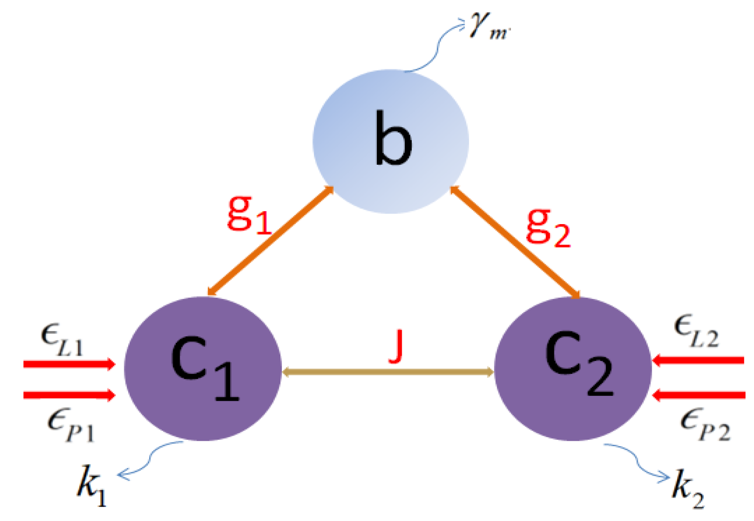
We consider a double-cavity optomechanical system [27], in which a common mechanical oscillator is coupled with the two cavities simultaneously as shown in Figure 1, where $c_i\left({\omega }_{ci}\right)$ represents the annihilation operator (frequency) of the $i\mathrm{t}\mathrm{h}$ cavity and $b\left({\omega }_m\right)$ denotes the annihilation operator and vibration frequency of the mechanical resonator. The set-up in Figure 1 can be realized in a Fabry–Pérot optical cavity, which is composed of two parallel mirrors separated by a certain distance. The standing wave can be produced in the optical cavity when we use an incident light field to drive the optical cavity. A partially transparent dielectric membrane is placed in the optical cavity, and it can be viewed as a mechanical oscillator under the interaction of radiation pressure. If the membrane oscillates around the node, the quadratic term of optomechanical coupling strength is much larger compared to the other terms. In addition, the membrane makes the system become a double-cavity system. Each cavity and mechanical resonator are coupled by optomechanical interactions of the form of quadratic coupling with the quadratic coupling constant of $g_i=\frac{{\partial }^2{\omega }_{ci}}{{\partial }^{2}q}\frac{x_0}{2}\left(i=1, 2\right)$. $p$ and $q$ represent the momentum operator and position operator of the mechanical resonator, respectively, and define the operator $P=\frac{x_0}{\hslash }p,Q=\frac{q}{x_0}$ under the condition of canonical quantization. Here,$\hslash$ is the Planck constant, $x_0=\sqrt{\frac{\hslash }{m{\omega }_m}}$ is the zero-point fluctuation of the mechanical resonator displacement, and P and $Q$ satisfy the relation of $[Q,P]=i$. In addition, the two cavities are coupled with a linear coupling constant $J$, and each cavity field is driven by a control field ${ϵ}_{Li}\left(i=1, 2\right)$ and a probe field ${ϵ}_{Pi}\left(i=1, 2\right)$ simultaneously. The model can be implemented in the membrane-in-the-middle optomechanical system. The Hamiltonian can be written as $\left(\hslash =1\right)$

$$\begin{array}{cc}\hfill \mathscr{H}=& {\omega }_{c1}{c}_1^{†}{c}_1+{\omega }_{c2}{c}_2^{†}{c}_2+\frac{1}{2}{\omega }_m\left(P^2+Q^2\right) \hfill \\ & +J\left(c_1^{†}{c}_2+c_2^{†}{c}_1\right)+2g_1{c}_1^{†}{c}_1{Q}^2+2g_2{c}_2^{†}{c}_2{Q}^2\hfill \\ & +i{ϵ}_{L1}\left(c_1^{†}{e}^{-i{\omega }_{L1}t}-c_1{e}^{i{\omega }_{L1}t}\right)+i{ϵ}_{L2}\left(c_2^{†}{e}^{-i{\omega }_{L2}t}-c_2{e}^{i{\omega }_{L2}t}\right)\hfill \\ & +i\left({ϵ}_{P1}{c}_1^{†}{e}^{-i{\omega }_{P1}t}-{ϵ}_{P1}^{*}{c}_1{e}^{i{\omega }_{P1}t}\right)+i\left({ϵ}_{P2}{c}_2^{†}{e}^{-i{\omega }_{P2}t}-{ϵ}_{P2}^{*}{c}_2{e}^{i{\omega }_{P2}t}\right).\hfill \end{array}$$

(1)

The Hamiltonian of the system is comprised of five terms, namely the free Hamiltonian of the two cavities, the free Hamiltonian of the mechanical oscillator, the interaction between the two cavities, the interaction between the mechanical oscillator and the two cavities, respectively, and the coupling terms between the control (probe) field and each cavity. In the rotating frame with the frequency ${\omega }_{Li}$, the Hamiltonian is written as

$$\begin{array}{cc}\hfill \mathscr{H}=& {\Delta }_1{c}_1^{†}{c}_1+{\Delta }_2{c}_2^{†}{c}_2+\frac{1}{2}{\omega }_m\left(P^2+Q^2\right) \hfill \\ & +J\left(c_1^{†}{c}_2+c_2^{†}{c}_1\right)+2g_1{c}_1^{†}{c}_1{Q}^2+2g_2{c}_2^{†}{c}_2{Q}^2\hfill \\ & +i{ϵ}_{L1}\left(c_1^{†}-c_1\right)+i{ϵ}_{L2}\left(c_2^{†}-c_2\right)\hfill \\ & +i\left({ϵ}_{P1}{c}_1^{†}{e}^{-i{\delta }_{1}t}-{ϵ}_{P1}^{*}{c}_1{e}^{i{\delta }_{1}t}\right)+i\left({ϵ}_{P2}{c}_2^{†}{e}^{-i{\delta }_{2}t}-{ϵ}_{P2}^{*}{c}_2{e}^{i{\delta }_{2}t}\right),\end{array}$$

(2)

where ${\Delta }_i={\omega }_{ci}-{\omega }_{Li}\left(i=1, 2\right)$ represents the detuning of the $i\mathrm{t}\mathrm{h}$ cavity mode relative to the $i\mathrm{t}\mathrm{h}$ control field and ${\delta }_i={\omega }_{Pi}-{\omega }_{Li}\left(i=1, 2\right)$ represents the detuning of the $i\mathrm{t}\mathrm{h}$ probe field relative to the $i\mathrm{t}\mathrm{h}$ control field. Using the Heisenberg–Langevin equations, the dynamics of the system [12,13,14,15,16] represented by Equation (2) can be described by the following set of equations:

$$\begin{array}{c}\dot{c_1}=-\left[\frac{k_1}{2}+i\left({\Delta }_1+2g_1{Q}^2\right)\right]c_1-iJ{c}_2+{ϵ}_{L1}+{ϵ}_{P1}{e}^{-i{\delta }_{1}t},\hfill \\ \dot{c_2}=-\left[\frac{k_2}{2}+i\left({\Delta }_2+2g_2{Q}^2\right)\right]c_2-iJ{c}_1+{ϵ}_{L2}+{ϵ}_{P2}{e}^{-i{\delta }_{2}t},\hfill \\ \dot{Q}={\omega }_{m}P,\hfill \\ \dot{P}=-{\omega }_{m}Q-4\left(g_1{c}_1^{†}{c}_1+g_2{c}_2^{†}{c}_2\right)Q-{\gamma }_{m}P.\hfill \end{array}$$

(3)

here, $k_i\left(i=1, 2\right)$ is the decay rate of the $i\mathrm{t}\mathrm{h}$ cavity mode and ${\gamma }_m$ is the damping rate of the mechanical oscillator. When the intensity of the control field is far greater than that of the probe field, the above operators can be written as the sum of the steady-state value and an additional fluctuation value, that is, $o=o_s+\delta o$, where $\mathrm{o}$ represents the following operators: $\left(c_1,c_2,P,Q\right)$. Substituting this expression into Equation (3), while ignoring the nonlinear terms, we obtain the linearized Heisenberg–Langevin equations and obtain the steady-state values of the system. The steady-state values can be written as

$$\begin{array}{c}{c}_{1s}=\frac{-iJ{ϵ}_{L2}+\left[\frac{k_2}{2}+i\left({\Delta }_2+2g_2{Q}_s^2\right)\right]{ϵ}_{L1}}{\left[\frac{k_2}{2}+i\left({\Delta }_2+2g_2{Q}_s^2\right)\right]\left[\frac{k_1}{2}+i\left({\Delta }_1+2g_1{Q}_s^2\right)\right]-J^2},\hfill \\ c_{2s}=\frac{-iJ{ϵ}_{L1}+\left[\frac{k_1}{2}+i\left({\Delta }_1+2g_1{Q}_s^2\right)\right]{ϵ}_{L2}}{\left[\frac{k_2}{2}+i\left({\Delta }_2+2g_2{Q}_s^2\right)\right]\left[\frac{k_1}{2}+i\left({\Delta }_1+2g_1{Q}_s^2\right)\right]-J^2},\hfill \\ P_s=0, Q_s=0.\hfill \end{array}$$

(4)

It can be seen from Equation (4) that for quadratic coupling, the steady-state value $Q_s$ of the position is 0, but the potential energy $\frac{1}{2}m{\omega }_m{Q}_s^2$ of the mechanical oscillator is not zero due to the thermal environment and zero-point fluctuations. Therefore, we define $X=Q^2,Y=P^2,Z=QP+PQ$ and, further, rewrite Equation (3) as follows

$$\begin{array}{c}\dot{c_1}=-\left[\frac{k_1}{2}+i({\Delta }_1+2g_{1}X)\right]c_1-iJ{c}_2+{ϵ}_{L1}+{ϵ}_{P1}{e}^{-i{\delta }_{1}t}, \hfill \\ \dot{c_2}=-\left[\frac{k_2}{2}+i({\Delta }_2+2g_{2}X)\right]c_2-iJ{c}_1+{ϵ}_{L2}+{ϵ}_{P2}{e}^{-i{\delta }_{2}t},\hfill \\ \dot{X}={\omega }_{m}Z,\hfill \\ \dot{Y}=-\left[{\omega }_m+4\left(g_1{c}_1^{†}{c}_1+g_2{c}_2^{†}{c}_2\right)\right]Z-2{\gamma }_{m}Y+{\gamma }_m\left(1+2n_{th}\right), \hfill \\ \dot{Z}=2{\omega }_{m}Y-2\left[{\omega }_m+4\left(g_1{c}_1^{†}{c}_1+g_2{c}_2^{†}{c}_2\right)\right]X-{\gamma }_{m}Z, \hfill \end{array}$$

(5)

where ${\gamma }_m\left(1+2n_{th}\right)$ is the constant introduced by the coupling between the mechanical oscillator and the thermal environment with $n_{th}={\left(e^{\frac{\hslash {\omega }_m}{k_{B}T}}-1\right)}^{-1}$ being the mean thermal phonon occupation number of the mechanical oscillator at temperature $T$. $k_B$ is the Boltzmann constant. Substituting $o=o_s+\delta o\left(o=c_1,c_2,X,Y,Z\right)$ into Equation (5), the steady-state values of the system can be expressed as

$$\begin{array}{c}{c}_{1s}=\frac{-iJ{ϵ}_{L2}+\left(\frac{{\kappa }_2}{2}+i{\mathsf{\Delta }}_2^{\prime }\right){ϵ}_{L1}}{\left(\frac{{\kappa }_2}{2}+i{\mathsf{\Delta }}_2^{\prime }\right)\left(\frac{{\kappa }_1}{2}+i{\mathsf{\Delta }}_1^{\prime }\right)-J^2},\hfill \\ c_{2s}=\frac{-iJ{ϵ}_{L1}+\left(\frac{{\kappa }_1}{2}+i{\mathsf{\Delta }}_1^{\prime }\right){ϵ}_{L2}}{\left(\frac{{\kappa }_2}{2}+i{\mathsf{\Delta }}_2^{\prime }\right)\left(\frac{{\kappa }_1}{2}+i{\mathsf{\Delta }}_1^{\prime }\right)-J^2},\hfill \\ Z_s=0,\hfill \\ X_s=\frac{{\omega }_m{Y}_s}{\left({\omega }_m+4g_1{c}_{1s}{c}_{1s}^{*}+4g_2{c}_{2s}{c}_{2s}^{*}\right)},\hfill \\ Y_s=\frac{1+2n_{th}}{2},\hfill \end{array}$$

(6)

where ${\mathsf{\Delta }}_i^{\prime }={\mathsf{\Delta }}_i+2g_i{X}_s\left(i=1, 2\right)$ is the effective detuning between the $i\mathrm{t}\mathrm{h}$ cavity mode and the $i\mathrm{t}\mathrm{h}$ control field. The quantum Langevin equations considering only the linear term of operator fluctuation can be written as:

$$\begin{array}{cc}\hfill \dot{\delta c_1}=& -\left(\frac{{\kappa }_1}{2}+i{\mathsf{\Delta }}_1^{\prime }\right)\delta c_1-2i{g}_1{c}_{1s}\delta X-iJ\delta c_2+{ϵ}_{P1}{e}^{-\mathrm{i}{\delta }_{1}t},\hfill \\ \hfill \dot{\delta c_2}=& -\left(\frac{{\kappa }_2}{2}+i{\mathsf{\Delta }}_2^{\prime }\right)\delta c_2-2i{g}_2{c}_{2s}\delta X-iJ\delta c_1+{ϵ}_{P2}{e}^{-\mathrm{i}{\delta }_{2}t},\hfill \\ \hfill \dot{\delta X}=& {\omega }_m\delta Z,\hfill \\ \hfill \dot{\delta Y}=& -\left[{\omega }_m+4\left(g_1{c}_{1s}{c}_{1s}^{*}+g_2{c}_{2s}{c}_{2s}^{*}\right)\right]\delta Z-2{\gamma }_m\delta Y, \hfill \\ \hfill \dot{\delta Z}=& 2{\omega }_m\delta Y-8X_s\left[\left(g_1{c}_{1s}\delta c_1^{†}+g_1{c}_{1s}^{*}\delta c_1\right)+\left(g_2{c}_{2s}^{*}\delta c_2+g_2{c}_{2s}\delta c_2^{†}\right)\right]\hfill \\ & -2\left[{\omega }_m+4\left(g_1{c}_{1s}{c}_{1s}^{*}+g_2{c}_{2s}{c}_{2s}^{*}\right)\right]\delta X-{\gamma }_m\delta Z.\hfill \end{array}$$

(7)

The system is not necessarily stable in some parameters, so it is necessary to judge the stability of the system under different conditions by solving the Rouse–Hurwitz stability criterion. The vector $V={\left(\delta Re\left[c_1\right],\delta Im\left[c_1\right],\delta Re\left[c_2\right],\delta Im\left[c_2\right],\delta X,\delta Y,\delta Z\right)}^T$ and $V_{in}={\left({ϵ}_{P1}\cos \left[{\delta }_{1}t\right],-{ϵ}_{P1}\sin \left[{\delta }_{1}t\right],{ϵ}_{P2}\cos \left[{\delta }_{2}t\right],-{ϵ}_{P2}\sin \left[{\delta }_{2}t\right],0,0,0\right)}^T$ are defined, and Equation (7) is expressed as the following matrix form:

$$\dot{V}=RV+V_{in}.$$

(8)

The coefficient matrix $R$ is given by

$$\left(\begin{array}{ccccccc}-\frac{{\kappa }_1}{2}& {\Delta }_1^{\prime }& 0& J& 0& 0& 0\\ -{\Delta }_1^{\prime }& -\frac{{\kappa }_1}{2}& -J& 0& 0& -2G_1& 0\\ 0& J& -\frac{{\kappa }_2}{2}& {\Delta }_2^{\prime }& 0& 2G_2\sin [\theta ]& 0\\ -J& 0& -{\Delta }_2^{\prime }& -\frac{{\kappa }_2}{2}& 0& -2G_2\cos [\theta ]& 0\\ 0& 0& 0& 0& -2{\gamma }_m& 0& -{\omega }_{m,eff}\\ 0& 0& 0& 0& 0& 0& {\omega }_m\\ -16G_1{X}_s& 0& -16G_2{X}_s\cos [\theta ]& -16G_2{X}_s\sin [\theta ]& 2{\omega }_m& -2{\omega }_{m,eff}& -{\gamma }_m\end{array}\right),$$

(9)

where $G_1=g_1\left|c_{1s}\right|=g_1{c}_{1s}{e}^{-i{\theta }_1}$ and $G_2=g_2\left|c_{2s}\right|=g_2{c}_{2s}{e}^{-i{\theta }_2}$ are the effective optomechanical coupling constants with the effective phase difference $\theta ={\theta }_2-{\theta }_1$, and ${\omega }_{m,eff}={\omega }_m+8\left(G_1^2/g_1\right)+8\left(G_2^2/g_2\right)$ is the effective mechanical oscillator frequency. From Equation (6), we can change the values of $c_{1s}$ and $c_{2s}$ by adjusting the amplitudes and phase of the control field, and then change the values of $G_1,G_2$ and $\theta$. Next, for simplicity, we make the value of $c_{1s}$ a real number through appropriately choosing the amplitudes and phase of the control field, that is, ${\theta }_1=0$. At this time, the effective phase difference $\theta ={\theta }_2$.

Supposing the solution of Equation (7) has the form $o=o_{+}{e}^{-\mathrm{i}\delta t}+o_{-}{e}^{\mathrm{i}\delta t}$, we set ${\mathsf{\Delta }}_1^{\prime }={\mathsf{\Delta }}_2^{\prime }={\mathsf{\Delta }}^{\prime },{\delta }_1={\delta }_2=\delta$. By comparing the coefficients of $-i\delta t$ and $i\delta t$, the solution of $\delta c_{1+}$ and $\delta c_{2+}$ can be given by

$$\begin{array}{c}\delta c_{1+}=\frac{\sqrt{k_2}{ϵ}_{p2}\left[\left(-iJ\right)\left(-A_1{M}_1+H_1\right)-A_1{\mathrm{e}}^{-i\theta }\right]+\sqrt{k_1}{ϵ}_{p1}\left[{\chi }_2\left(-H_1+A_1{M}_1\right)+A_1\frac{G1}{G2}\right]}{\left(-A_1{M}_1+H_1\right)A_2-A_1{H}_2}, \hfill \\ \delta c_{2+}=\frac{\sqrt{k_1}{ϵ}_{p1}\left[\left(-iJ\right)\left(-A_1{M}_1+H_1\right)-A_1{\mathrm{e}}^{i\theta }\right]+\sqrt{k_2}{ϵ}_{p2}\left[{\chi }_1\left(-H_1+A_1{M}_1\right)+A_1\frac{G1}{G2}\right]}{\left(-A_1{M}_1+H_1\right)A_2-A_1{H}_2},\hfill \end{array}$$

(10)

with

$$\begin{array}{c}{\chi }_1=-\left(\frac{k_1}{2}+i{\mathsf{\Delta }}_1^{\prime }\right)+i\delta ,{\chi }_{11}=-\left(\frac{k_1}{2}-i{\mathsf{\Delta }}_1^{\prime }\right)+i\delta , \hfill \\ {\chi }_2=-\left(\frac{k_2}{2}+i{\mathsf{\Delta }}_2^{\prime }\right)+i\delta ,{\chi }_{22}=-\left(\frac{k_2}{2}-i{\mathsf{\Delta }}_2^{\prime }\right)+i\delta , \hfill \\ A_1={\chi }_{11}{\chi }_{22}+J^2,A_2={\chi }_1{\chi }_2+J^2, \hfill \\ H_1={\chi }_{11}\frac{G_2}{G_1}+{\chi }_{22}\frac{G_1}{G_2}-2iJcos\left[\theta \right],H_2={\chi }_1\frac{G_1}{G_2}+{\chi }_2\frac{G_2}{G_1}+2iJcos\left[\theta \right], \hfill \\ M_1=\frac{\left(-2{\gamma }_m+i\delta \right)\left(-{\gamma }_m+i\delta \right)\left(i\delta \right)+2\left(-{\gamma }_m+i\delta \right){\omega }_m{\omega }_{m,eff}}{16i\left(-2{\gamma }_m+i\delta \right)G_1{G}_2{\omega }_m{X}_s}. \hfill \end{array}$$

The input–output relation of the optomechanical system can be written as

$$\begin{array}{c}{ϵ}_{p1}^{out}+{ϵ}_{p1}^{in}{e}^{-i{\delta }_{1}t}=\sqrt{{\kappa }_1}\delta c_1,\\ {ϵ}_{p2}^{out}+{ϵ}_{p2}^{in}{e}^{-i{\delta }_{2}t}=\sqrt{{\kappa }_2}\delta c_2.\end{array}$$

(11)

Here, ${ϵ}_{p1}^{in}=\frac{{ϵ}_{p1}}{\sqrt{{\kappa }_1}},{ϵ}_{p2}^{in}=\frac{{ϵ}_{p2}}{\sqrt{{\kappa }_2} }$. Next, assuming that the output field also has the form of $o=o_{+}{e}^{-\mathrm{i}\delta t}+o_{-}{e}^{\mathrm{i}\delta t}$, by comparing the coefficients of $-i\delta t$ and $i\delta t$, the relations are obtained as follows:

$$\begin{array}{c}{ϵ}_{p1+}^{out}=\sqrt{{\kappa }_1}\delta c_{1+}-\frac{{ϵ}_{p1}}{\sqrt{{\kappa }_1}},{ϵ}_{p1-}^{out}=0,\\ {ϵ}_{p2+}^{out}=\sqrt{{\kappa }_2}\delta c_{2+}-\frac{{ϵ}_{p2}}{\sqrt{{\kappa }_2}},{ϵ}_{p2-}^{out}=0.\end{array}$$

(12)

Transmission amplitudes can be expressed as [27]:

$$\begin{array}{c}{T}_{12}={\left|\frac{{ϵ}_{p2+}^{out}}{{ϵ}_{p1}^{in}}\right|}_{{ϵ}_{p2}^{in}=0},\\ T_{21}={\left|\frac{{ϵ}_{p1+}^{out}}{{ϵ}_{p2}^{in}}\right|}_{{ϵ}_{p1}^{in}=0}.\end{array}$$

(13)

So, by substituting Equation (10) into Equations (12) and (13), transmission amplitudes can be obtained as

$$\begin{array}{c}{T}_{12}=\left|\frac{\sqrt{k_1{k}_2} \left[\left(-iJ\right)\left(-A_1{M}_1+H_1\right)-A_1{\mathrm{e}}^{i\theta }\right]}{\left(-A_1{M}_1+H_1\right)A_2-A_1{H}_2}\right|,\hfill \\ T_{21}=\left|\frac{\sqrt{k_1{k}_2} \left[\left(-iJ\right)\left(-A_1{M}_1+H_1\right)-A_1{\mathrm{e}}^{-i\theta }\right]}{\left(-A_1{M}_1+H_1\right)A_2-A_1{H}_2}\right|.\hfill \end{array}$$

(14)

3. Results and Discussions about Nonreciprocity

From Equation (14), we can find that transmission amplitudes ($T_{12}$ and $T_{21}$) are related to the effective phase difference $\theta$. The reason why the system produces a nonreciprocal response is that different transmission paths interfere with each other. For example, the input signal from $c_1$ can be transmitted to ${\mathrm{c}}_2$ through two paths: path 1 ($c_1\to \mathrm{b}\to c_{2 }$) and path 2 $(c_1\to c_2$). 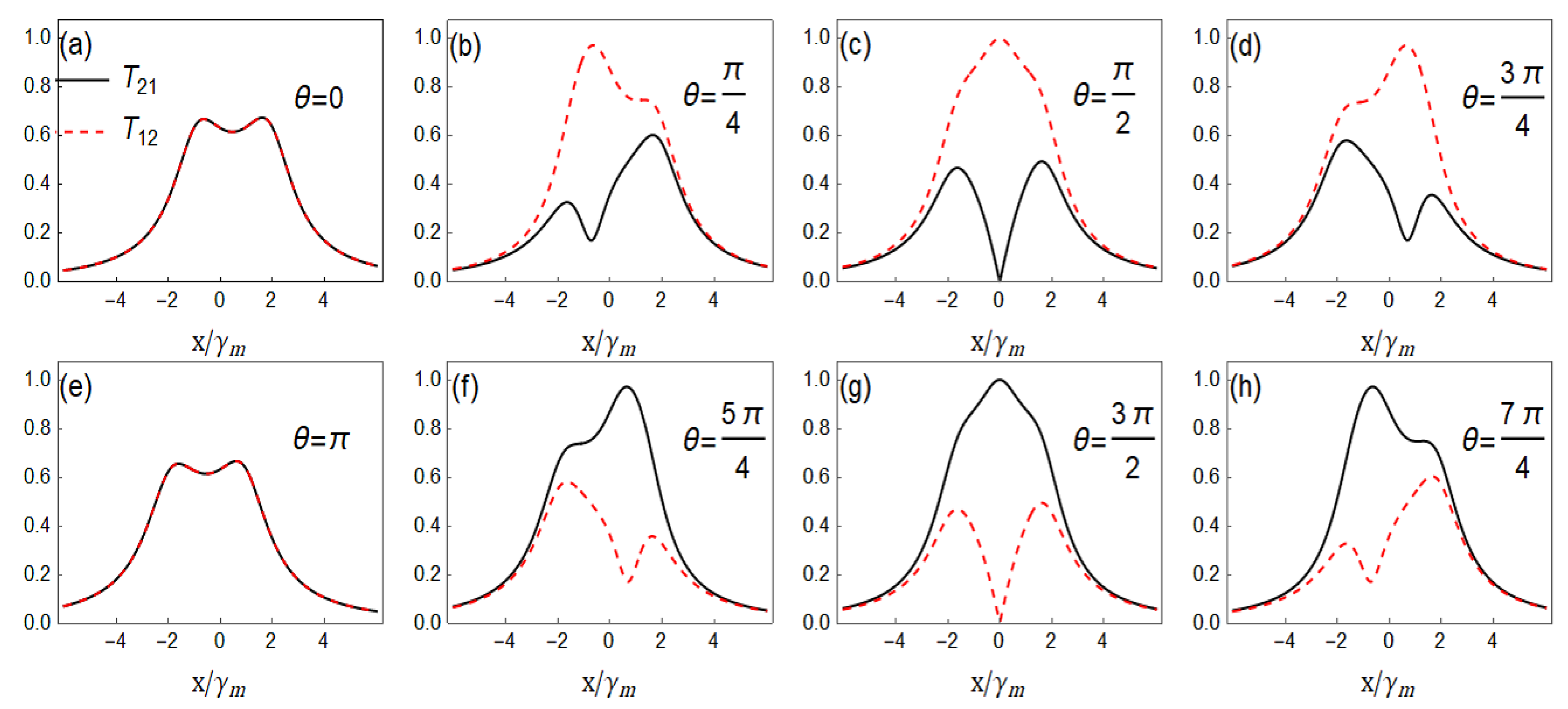In path 2, $G_1$,$G_2$ and $J$ play the major role in this process. In the following discussions, to study the influence of effective phase difference $\theta$ on nonreciprocity, we fix a series of parameters $\left( k_1=k_2=k,{\mathsf{\Delta }}^{\prime }=2{\omega }_m,n_{th}=0.5,k=2{\gamma }_m,{\omega }_m=10{\gamma }_m, {\omega }_{m,eff}=1.01{\omega }_m,J=1{\gamma }_m,G_1=G_2=\frac{1}{2}{\gamma }_m\right)$ and plot the variation of transmission amplitudes ($T_{12}$ and $T_{21}$) with standardized detuning $\frac{x}{{\gamma }_m}\left( x=\delta -2{\omega }_m\right)$ in different effective phase difference $\theta$. As shown in Figure 2, when $\theta =n\pi$, transmission amplitudes $T_{12}=T_{21}$, and the system is reciprocal. When $\theta \ne n\pi$, transmission amplitudes $T_{12}\ne T_{21}$, and the system is nonreciprocal. When $\theta =\frac{\pi }{2}$ and $\theta =\frac{3\pi }{2}$, the transmission direction of the system is reserved. In the case $\theta =\frac{\pi }{2}+n\pi$, the spectral line is symmetrical about the axis $\frac{x}{{\gamma }_m}=0$. In the range of $0<\theta <\pi$, transmission amplitudes $T_{12}>T_{21}$, and in the case of $\pi <\theta <2\pi$, transmission amplitudes $T_{12}<T_{21}$. Therefore, the phase difference will not only affect the magnitude of nonreciprocal response, but also affect the direction of nonreciprocal response.

Next, the perfect nonreciprocity under the condition with red detuning $({\mathsf{\Delta }}_i^{\prime }=2{\omega }_m, x=\delta -2{\omega }_m)$ or blue detuning $({\mathsf{\Delta }}_i^{\prime }=-2{\omega }_m,x=\delta +2{\omega }_m)$ is discussed, respectively. The perfect nonreciprocity means that we can realize the transmission process with $T_{12}=1,T_{21}=0$ or with $T_{12}=0,T_{21}=1$. In the following discussion, only one of the above two processes will be considered. At this time, the signal can be completely transmitted from $c_1$ to $c_2$, but it cannot be completely transmitted from $c_2$ to $c_1$, which can realize unidirectional transmission of the signal, namely

$$\begin{array}{c}{T}_{12}=1,\\ T_{21}=0.\end{array}$$

(15)

According to Equation (15), we obtain

$$\begin{array}{c}\left(-iJ\right)\left(-A_1{M}_1+H_1\right)=A_1{e}^{-i\theta },\\ \left|\frac{2J\sqrt{k_1{k}_2}sin\left[\theta \right]}{A_2{e}^{-i\theta }+iJ{H}_2}\right|=1.\end{array}$$

(16)

When $\theta =\frac{\pi }{2}$ and the system is in red detuning $\left({\mathsf{\Delta }}^{\prime }=2{\omega }_m\right)$, by solving the above equation, we obtain

$$\begin{array}{cc}\hfill J& =\frac{1}{2}\sqrt{k_1{k}_2} , \frac{G_2^2}{G_1^2}=\frac{k_2}{k_1}\left(x=0\right) \hfill \\ \hfill G_1& =\frac{\sqrt{k_1{\omega }_{m,eff}\left({\gamma }_m\left(k_1{k}_2-32{\omega }_m^2\right)U_1+4\left(k_1+k_2\right){\omega }_m{U}_2\right)}}{2\sqrt{2}\sqrt{2\left(1+2n_{th}\right)\left(k_1{k}_2-16{\omega }_m^2\right){\omega }_m\left({\gamma }_m^2+{\omega }_m^2\right)}}\hfill \\ & =\frac{\sqrt{k_1{\omega }_{m,eff}\left(4\left(k_1+k_2\right){\gamma }_m{\omega }_m{U}_1-\left(k_1{k}_2-32{\omega }_m^2\right)U_2\right)}}{2\sqrt{2}\sqrt{8\left(1+2n_{th}\right)\left(k_1+k_2\right){\omega }_m^2\left({\gamma }_m^2+{\omega }_m^2\right)}},\hfill \end{array}$$

(17)

With $U_1={\gamma }_m^2+{\omega }_m\left({\omega }_{m,eff}+{\omega }_m\right)$, $U_2=-2{\omega }_m\left({\gamma }_m^2+{\omega }_m^2\right)+{\omega }_{m,eff}\left({\gamma }_m^2+2{\omega }_m^2\right)$. It can be obtained that the perfect nonreciprocity appears at the resonance frequency $\left(x=0\right)$. The coupling constant $J$ satisfying the perfect nonreciprocal condition is related to the decay rates $k_1$ and $k_2$ of the cavity, and satisfies the condition $J=\frac{1}{2}\sqrt{k_1{k}_2}$. 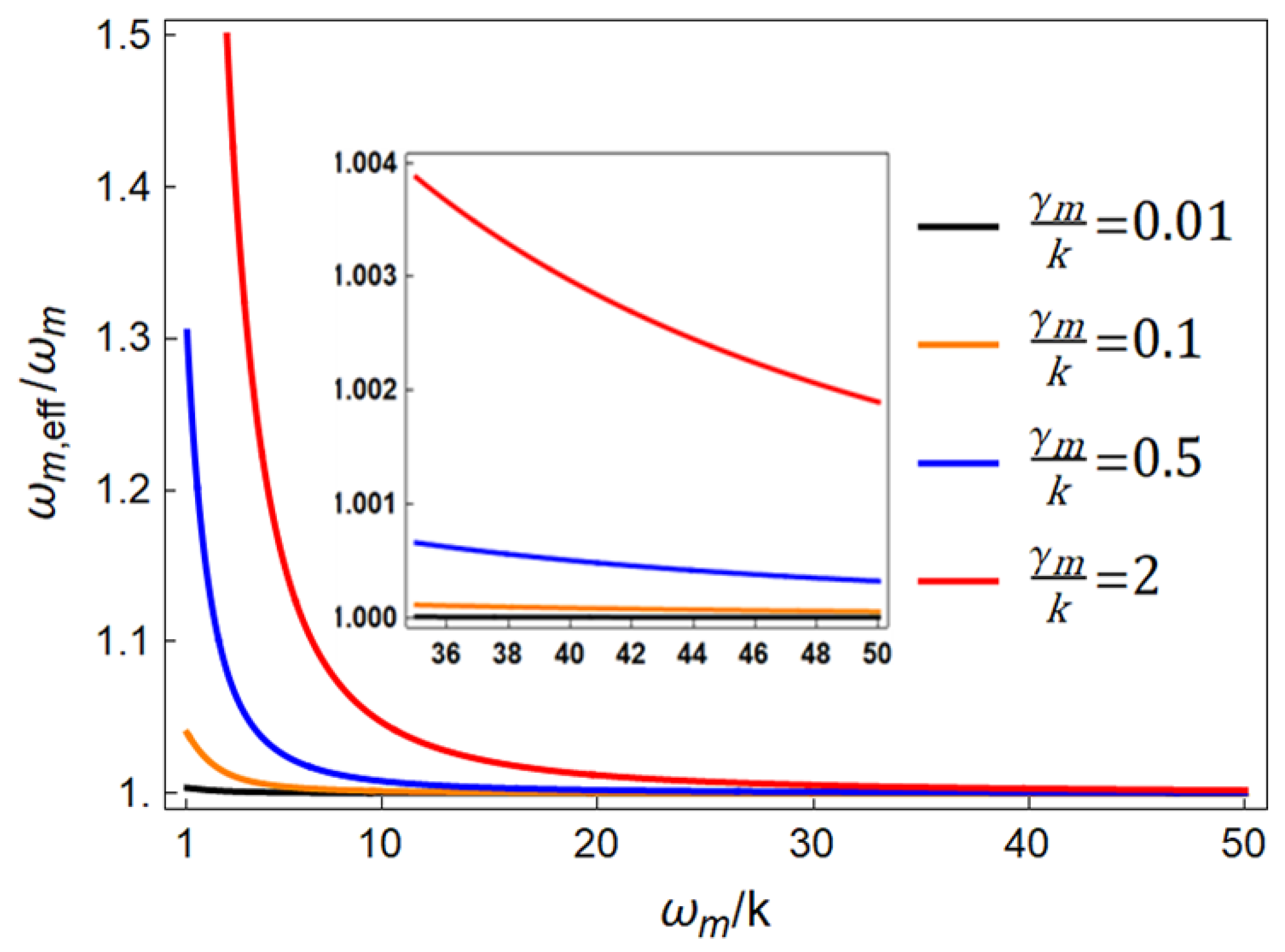At the same time, it is obvious that the value of $G_i\left(i=1, 2\right)$ is related to a series of parameters ($k_i,{\gamma }_m,{\omega }_m,{\omega }_{eff},n_{th}$), which must satisfy both expressions of $G_i$ in Equation (17) simultaneously. As Figure 3 shows, when $k_1=k$ and $k_2=10k$, with the increase in ${\omega }_m$, the ratio of the effective mechanical oscillator frequency ${\omega }_{m,eff}$ to the mechanical oscillator frequency ${\omega }_m$ gradually approaches 1.

Assuming that ${\omega }_m$ is much larger than other parameters, the effective mechanical oscillator frequency ${\omega }_{m,eff}\approx {\omega }_m$ is approximately considered. For the value of $G_i\left(i=1,2\right)$, only the highest power of ${\omega }_m$ and its previous coefficients are retained; thus, $J=\frac{1}{2}\sqrt{k_1{k}_2},G_1\approx \frac{\sqrt{k_1{\gamma }_m}}{2\sqrt{1+2n_{th}}}$ and $G_2\approx \frac{\sqrt{k_2{\gamma }_m}}{2\sqrt{1+2n_{th}}}$ are obtained. Substituting the above conditions into Equation (14) shows that although $G_i$ satisfying perfect nonreciprocity is related to the mean thermal phonon occupation number $n_{th}$, the value of $n_{th}$ has no influence on the final transmission amplitude under this condition, so the value of $n_{th}$ is arbitrary. In the case of red detuning, compared with the condition $(J=\frac{1}{2}\sqrt{k_1{k}_2},G_i=\frac{\sqrt{k_i{\gamma }_m}}{2})$ that the double optomechanical systems with linear coupling should achieve perfect nonreciprocity under when $\theta =\frac{\pi }{2}$, the value of $G_i$ of the double optomechanical systems with quadratic coupling is related to $n_{th}$, and the value of $n_{th}$ can be controlled by temperature $T$, so the $G_i$ can achieve perfect nonreciprocity at different values by controlling temperature $T$. 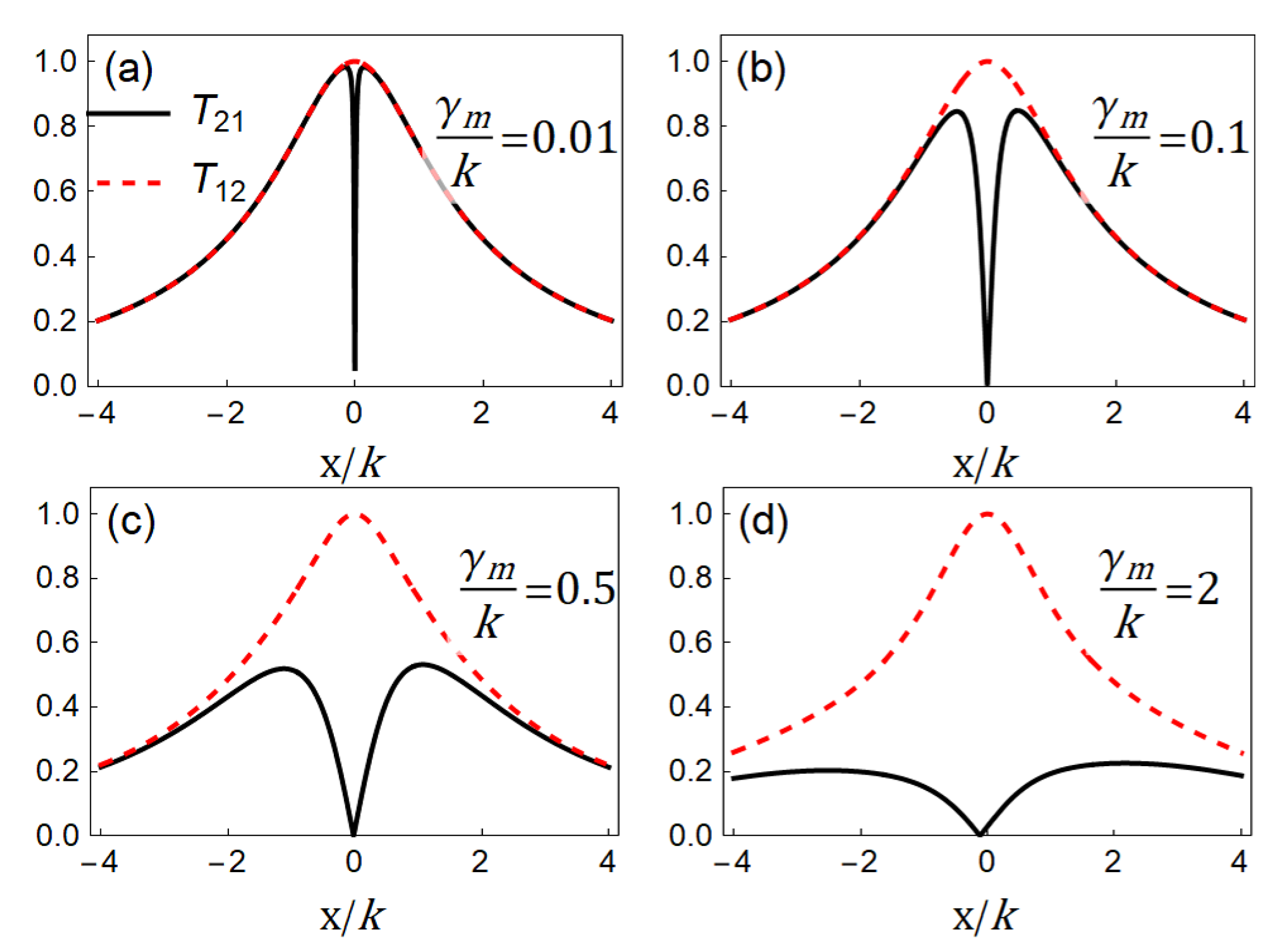Under the above conditions, the relationship between transmission amplitudes ($T_{12}$ and $T_{21}$) and normalized detuning $\frac{x}{k}$ at different $\frac{{\gamma }_m}{k}$ is shown in Figure 4, in which the other parameters are taken as $k_1=k,k_2=10k,{\omega }_m=40k,{\omega }_{m,eff}={\omega }_m$ and the values of $\frac{{\gamma }_m}{k}$ are 0.01, 0.1, 0.5 and 2, in turn. Under the conditions that $k_1$ and $k_2$ are fixed, and $J$ is also fixed, as ${\gamma }_m$ takes different values, the values of $G_1$ and $G_2$ will change, but $G_2=\sqrt{10}{G}_1$ is always true. It can be seen from Figure 4 that when $\frac{{\gamma }_m}{k}$ is relatively small, the spectral line width of transmission amplitude $T_{21}$ is proportional to the damping rate of the mechanical oscillator $\left(△{\omega }_m\propto {\gamma }_m\right)$ and perfect nonreciprocity can be achieved even when ${\gamma }_m$ is very small. With the increase in ${\gamma }_m$, it leads to the increase in $G_i$, and the effective optomechanical coupling constant $G_i$ begins to play a major role in the signal transmission process, and the range of nonreciprocity increases accordingly.

Next, we consider that the system is in the case with $\theta =-\frac{\pi }{2}$ and blue detuning $({\mathsf{\Delta }}_i^{\prime }=-2{\omega }_m)$. When ${\omega }_m$ is much larger than other parameters, Equation (16) can be solved in a similar way to the previous case of the red detuning, and only the highest power of ${\omega }_m$ and the previous coefficient can be retained for the values of $G_i$ and $J$, so that $J_{\pm }=\frac{\left(3\pm 2\sqrt{2}\right)\sqrt{k_1{k}_2}}{2},G_{1\pm }\approx \frac{\sqrt{3\pm 2\sqrt{2}}\sqrt{k_1{\gamma }_m}}{2\sqrt{1+2n_{th}}}$ and $G_{2\pm }\approx \frac{\sqrt{3\pm 2\sqrt{2}}\sqrt{k_2{\gamma }_m}}{2\sqrt{1+2n_{th}}}$ can be obtained. Perfect nonreciprocity is also obtained at resonance frequency $\left(x=0\right)$. In the case of blue detuning, $G_i$ is related to the mean thermal phonon occupation number $n_{th}$, which is same as in the case of red detuning, but the value of $n_{th}$ has no effect on the final transmission amplitudes, so $G_i$ can realize the perfect nonreciprocity at different values by controlling the temperature $T$. 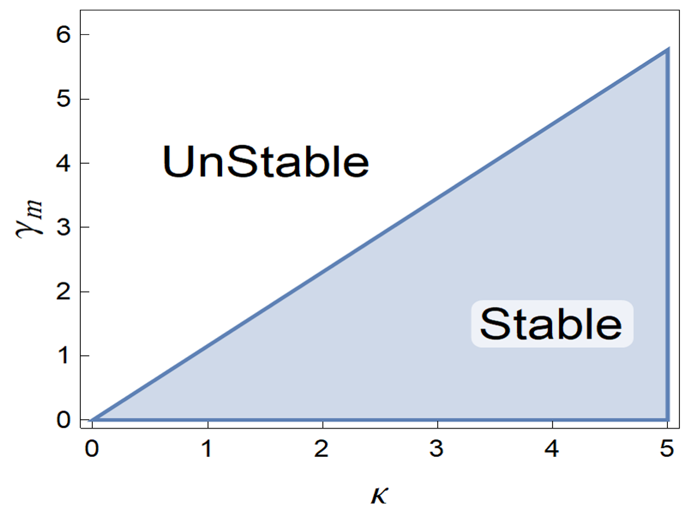By solving the Rouse–Hurwitz stability criterion, we obtain that when $J=J_{-}$ and $G=G_{-}$, the system is always stable. When $J=J_{+}$ and $G=G_{+}$, the system is stable only when it meets the conditions shown in Figure 5.

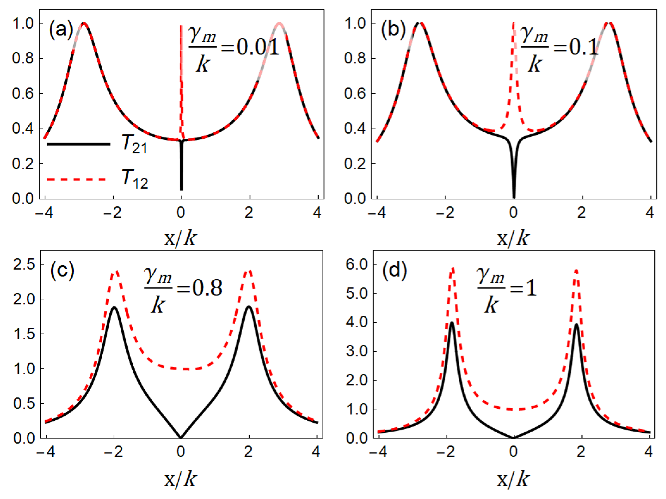
In Figure 6a–d, the values of the parameters are the same as those shown in Figure 5, and we plot the relationship between transmission amplitudes ($T_{12}$ and $T_{21}$) and normalized detuning $\frac{x}{k}$ at different $\frac{{\gamma }_m}{k}$. The values of $\frac{{\gamma }_m}{k}$ are taken as 0.01, 0.1, 0.8 and 1, in turn. When $J=J_{+}$ and $G=G_{+}$, it can be seen from Figure 5 that the system is unstable in the range of ${\gamma }_m>1.16k$. From Figure 6c,d, where $\frac{{\gamma }_m}{k}=$ 0.8 and 1, the system is close to the critical state of stability and instability. In this case, the system displays a gain phenomenon for the probe field. The occurrence of gain is due to nonlinear effects based on the quantum coherence, which means optomechanically induced amplification [31] takes place. At this moment, the peak value of transmission amplitude is far greater than 1. In addition, the spectral line of $T_{12}$ is multi-peak. As shown in Figure 6a, when $\frac{{\gamma }_m}{k}$ is small, the spectrum width of transmission amplitude is proportional to the attenuation rate ${\gamma }_m$ of the mechanical oscillator. Excluding the extremely small range around $x=0$, transmission amplitude $T_{12}=T_{21}$, which means the processes of transmission are reciprocal.

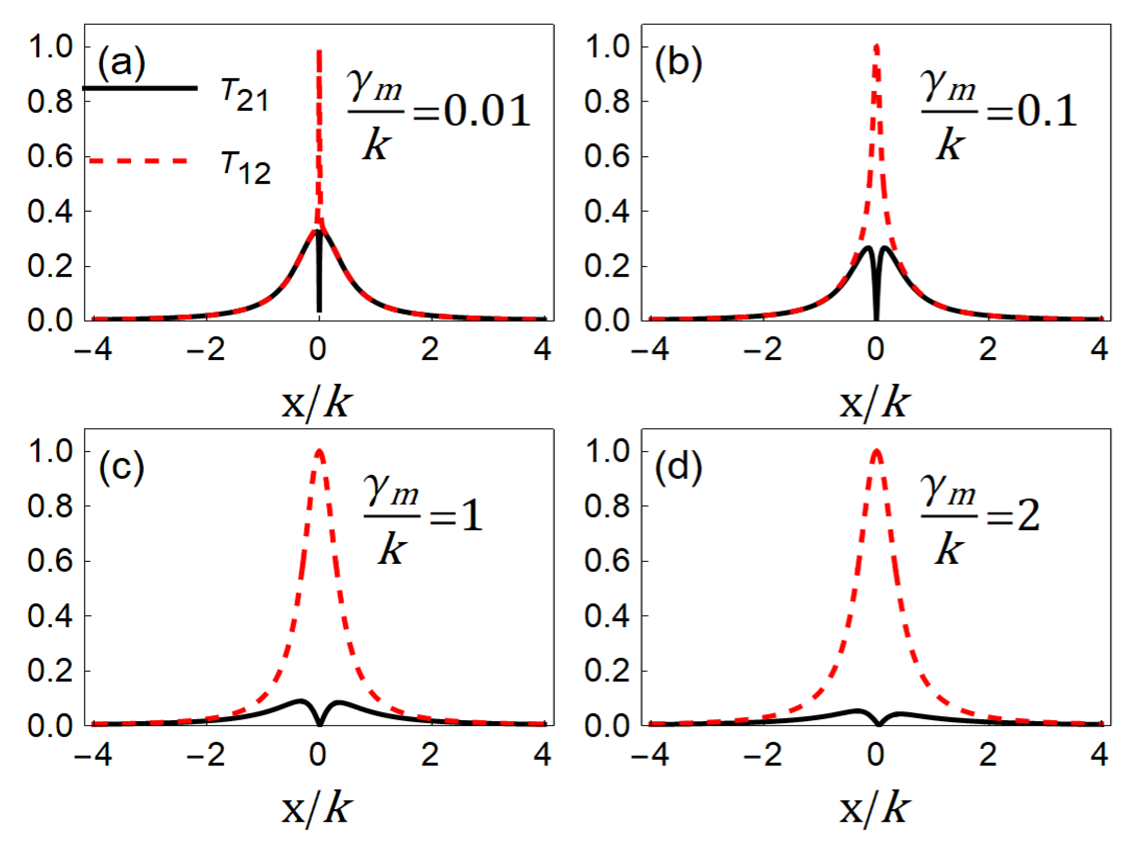
Finally, we make $J=J_{-},G=G_{-}$ and let $\frac{{\gamma }_m}{k}$ equal 0.01, 0.1, 1 and 2, in turn. The other parameters are the same as those in Figure 6. As shown in Figure 7, with the increase in $\frac{{\gamma }_m}{k}$, the maximum value of $T_{21}$ gradually decreases and the spectral line width of $T_{12}$ gradually increases, which means that the range of nonreciprocal response becomes larger. However, due to the system being stable in the whole range, there will be no transmission amplitudes greater than 1, and multi-peaked spectral lines and perfect nonreciprocity can be achieved at the resonance frequency $\left(x=0\right)$.

4. Conclusions

In sum, we study the optical nonreciprocity of double optomechanical systems with quadratic coupling and find that the magnitude and direction of the nonreciprocity of the system can be changed by adjusting the nonreciprocal phase difference $\theta$. At the same time, it is calculated that when the system is in red detuning with $\theta =\frac{\pi }{2}$ and ${\omega }_m$ is much larger than other parameters, there is a group of $G_i$ and $J$ that meet the conditions of perfect nonreciprocity. When the system is in blue detuning with $\theta =-\frac{\pi }{2}$ and ${\omega }_m$ is much larger than other parameters, there are two groups of $G_i$ and $J$ that can achieve perfect nonreciprocity. Specifically, the system is not always stable under some parameters, one of which causes the maximum value of transmission amplitudes to be far greater than 1 in a certain range. In the case of $\theta =\pm \frac{\pi }{2}$ and ${\mathsf{\Delta }}_i^{\prime }=\pm 2{\omega }_m$, the perfect nonreciprocity is obtained at the resonance frequency $\left(x=0\right)$, whether the system is in red or blue detuning. When other parameters are fixed, the ratio of $\frac{{\gamma }_m}{k}$ can affect the magnitude and range of nonreciprocity. In addition, we compare the conditions of realizing perfect nonreciprocity between the double optomechanical systems with linear coupling and the double optomechanical systems with quadratic coupling and find that when the decay rate $k_i$ of the cavity mode and the damping rate ${\gamma }_m$ of the mechanical oscillator are fixed, both of them satisfy the same relation for the value of $J$. However, the value of effective optomechanical coupling constant $G_i$ is different and is not only related to $k_i$ and ${\mathsf{\gamma }}_{\mathrm{m}}$ but also related to $n_{th}$, where the value of $n_{th}$ will not affect the transmission amplitudes. Therefore, compared with the double optomechanical systems with linear coupling, the double optomechanical systems with quadratic coupling can change the value of $G_i$ and achieve perfect nonreciprocity by keeping the system at different temperatures $T$. In addition, we discuss the three-mode optomechanical system where the coupling between the cavity field and the mechanical oscillator is in the quadratic case. Comparing with the Ref. [27] in which optical nonreciprocity in three-mode optomechanical systems with linear coupling is investigated, we extend their model to the case with quadratic coupling. The Hamiltonian of the linear coupling is proportional to $c_1^{†}{c}_{1}Q$, which means the linear coupling denotes work done by light pressure pushing the oscillator to displacement $Q$. The Hamiltonian of the quadratic coupling, by contrast, is proportional to $c_1^{†}{c}_1{Q}^2$, which means the quadratic coupling will change the native frequency of the oscillator. In order to achieve optical nonreciprocity, these two different couplings have different requirements for selections of physical parameters. For the linear coupling, the effective detuning needs to be equal to native frequency ${\omega }_m$ of the oscillator [27]. However, for the quadratic coupling in our model, the condition that the effective detuning is equal to ${\omega }_m$ will be broken. Here, the realization of optical nonreciprocity requires the effective detuning with $2{\omega }_m$. We know that production of these two different kinds of coupling depends on the position of the oscillator. Our studies show that the three-mode optomechanical systems with quadratic coupling can also be used as an alternative scheme for producing optical nonreciprocity.