Abstract
Light wave reflection intensity from optical disordered media is associated with its phase, and the phase statistics influence the reflection statistics. A detailed numerical study is reported for the statistics of the reflection coefficient and its associated phase for plane electromagnetic waves reflected from one dimensional Gaussian white-noise optical disordered media, ranging from weak to strong disordered regimes. The full Fokker–Planck (FP) equation for the joint probability distribution in the space is simulated numerically for varying length and disorder strength of the sample; and the statistical optical transport properties are calculated. Results show the parameter regimes of the validation of the random phase approximations (RPA) or uniform phase distribution, within the Born approximation, as well as the contribution of the phase statistics to the different reflections, averaging from nonuniform phase distribution. This constitutes a complete solution for the reflection phase statistics and its effect on light transport properties in a 1D Gaussian white-noise disordered optical potential.
1. Introduction
Wave propagation through 1D disordered media has been a subject of study for both optical and electrical systems. Typical physical examples of these problems are light transport in random dielectric media, electron transport in disordered conductors, etc. [,,,,,,]. Most of the transport reported results are within the random phase approximations (RPA) or uniform phase distribution, however, the contribution of the phase statistics to the different reflection averaging from nonuniform phase distribution is not well studied. Disordered 1D systems are quite generic as regards their transport properties which are well addressed first in electronic systems—disordered 1D conductors are all alike, but every ordered 1D conductor is ordered in its own way.
For electronic systems, quantum interference effects are important at low temperatures, when de-coherence due to the inelastic process may be neglected. At low enough temperatures with static disorder, the transport properties of the electronic systems are highly fluctuating (i.e., sample specific) due to the different conductors with the same impurity concentration but with different microscopic arrangements of the impurities, which can differ substantially in their transport properties. It is shown that the root mean-square-fluctuation is more than the average for length scales larger than the scattering mean free path (i.e., localization length), while for the length scales within the mean free path (i.e., in the good metallic regime for quasi 1D and higher dimensional systems) the fluctuations are finite and universal, the so-called universal conductance fluctuations (UCF) []. These fluctuations make the resistance and the conductance non-self-averaging quantities for electronic systems. The resistance at low temperatures when quantum effects are important is non-Ohmic, i.e., nonadditive in series. The non-additive nature arises because of the non-local effects of the quantum wave amplitudes associated with the electron in the conductor.
In the case of optical disordered media, similar phenomena happen to the light or photonics waves for the reflection coefficient, which could be thought of as optical resistance. However, the reflection coefficient of an optical 1D system is bounded by the maximum reflection coefficient of the value one. Due to this limitation, it will be shown later that the effect of non-self-averaging is implied in the fact that the average and fluctuations for the reflection coefficient both increase in a similar way to the electronic case, with fluctuation higher than the average. Therefore, one must take proper account of the phase for addition of the two optical samples. In this case, to calculate any meaningful average quantity for a non-self-averaging quantity, such as the reflection (for optical case) coefficient, resistance, and the conductance (for electronic cases), one should know the full probability distribution of the same for every length of the sample. The derivation of the Fokker–Planck (FP) equation for the full probability distribution of the reflection amplitude and its associated phase for the Gaussian white noise disordered optical or electronic media have been reported [,,,,,,]. Exact results for the average of different moments of the electronic conductance can be calculated analytically for the weak-disorder case using the Fokker–Planck equation only within the random phase approximation (RPA) (i.e., uniform phase distribution) for white noise disorder. However, for the optical case, the FP equation is not closed in the reflection coefficient within the RPA and can be solved only with the limit of weak disorder and weak reflection. The approximation made in the weak disorder case is that the phase of the complex reflection amplitude relative to the incident wave, (or the relative phase of two electronic/optical conductors), are distributed uniformly, which is the random phase approximation (RPA). The analytical results for electronic cases show that the resistance and the conductance have log-normal distributions for large sample lengths [,,,]. Similar things could be defined in the optical case. It is difficult to get an average quantity by direct analytical calculation for larger sample length which includes the nonuniform, complicated phase distribution, where the phase distribution depends on the strength of the disorder and length of the sample. However, the actual validity of the random phase approximation has not been studied in detail for varying disorder strength and sample length. Additionally, the effect of the phase distributions on the reflection coefficients was also not systematically addressed earlier. There are issues, such as the actual contribution of the nonuniform phase distribution to the different transport averaging processes, that have not been well studied so far.
In this paper, we study numerically the joint probability distribution P(r, θ) of the phase (θ) and the reflection coefficient (r) of the complex amplitude reflection coefficient (R(L) = √r exp(iθ)) for one-dimensional optical disordered media with the Gaussian white noise disorder, for different lengths of the sample and different disorder strengths. The large parameter space of the light reflection was explored. In particular, we simulate a solution of the Fokker–Planck equation, where the probability density is varying in the (r, θ)-space and evolving with the sample length L, with different disorder strengths. Using the invariant imbedding technique, a non-linear Langevin equation can be derived for the complex R(L). Then, using the stochastic Liouville equation for the probability evolution and the Novikov theorem to integrate out the stochastic aspect due to the random potential, one gets the Fokker–Planck (FP) equation in the (r, θ)-space for varying sample length L [,]. Integrating θ and r parts separately from the joint probability distribution P(r, θ), we have calculated the marginal probability distributions P(r) and P(θ) for r and θ, respectively, for a given length and disorder strength of the sample. The validity of the random phase approximation has been outlined for the parameters on which the phase distribution depends, namely the sample length, scattering mean free path/localization length, and the wave vector of the incoming wave. The effect of the disorder on random phase approximation is analyzed, and averages and the fluctuations are calculated for the reflection coefficients with different types of phase distributions associated with the disorder strength parameter of the optical samples. To the best of our knowledge, this is the first work where the joint probability distributions for the reflection coefficient and its phase for a 1D Gaussian white-noise disordered reflector are calculated for all length scales and for different disorder strengths, a complete visualization and quantification of the reflection probability for 1D disordered media. The way we have calculated the different quantities here involves essentially no approximations (within the numerical accuracy). We report mainly the results of the light transport in random dielectric media (or, random layered media), but as discussed, the formalism applies equally well to the case of electronic transport in disorder conductors via Landauer formalism, and this shows that the phase statistics of the reflection coefficient and the phase associate with resistance/conductance are same [].
2. Materials and Methods
2.1. Langeving and Fokker–Planck Equations for Complex R(L)
The Maxwell’s equations can be transformed to the Helmholtz equation (wave equation), for both E and H fields. Consider the E part of the electromagnetic (EM) wave equation in scalar, polarization conserved, in a dielectric media with . Then E field in 1D is given as:
Transforming the EM wave equation in E to the standard Helmholtz equation form, we obtain:
where and , with is the constant dielectric background and is the spatially fluctuating part of the dielectric medium. Derivation of the Langevin and Fokker–Planck equations have been reported earlier, however, for the completeness of numerical simulation of this paper, we will describe this in brief below.
Consider a plane wave of wave vector k is incident from the right side of the disordered sample of length having the reflection amplitude . The non-linear Langevin equation for the reflection amplitude for the plane wave scattering problem can be derived by the invariant imbedding technique. The Langevin equation for the complex amplitude reflection coefficient can be derived [,,,,]:
with the initial condition R(L) = 0 for L = 0.
The Langevin equation can be used to derive a FP equation for the reflection probability density. To get the Fokker–Planck equation from the non-linear Langevin equation, the probability density equation is first derived and then the stochastic aspect due to the random potential is integrated out. The Langevin equation (i.e., Equation (3)) can be solved analytically for the Gaussian white noise potential to get the FP equation. Detailed derivation steps have been reported in several places, however, it is worth repeating here some essential steps of the calculations for completeness of the numerical method []. The non-linear Langevin equation for in (Equation (3)) is two coupled differential equations for the magnitude and the associated phase parts. Now, taking
and substituting Equation (4) into Equation (3), and equating the real and the imaginary parts on both sides of Equation (3), one gets two coupled differential equations,
Now, according to the van-Kampen lemma [], these two stochastic coupled differential equations will produce a flow of the density Q(r, θ) in the (r, θ)-space and will obey the stochastic Liouville equation with increasing length of the sample, i.e., Q(r, θ) is the solution of the stochastic Liouville equation:
where and are given by Equations (5) and (6). Now, substituting the values of and in Equation (7) one gets:
To obtain the Fokker–Planck equation, Equation (8) is averaged over the stochastic aspect, i.e., over all realizations of the random potential. For the case of a Gaussian white noise potential, Equation (8) can be averaged out over the stochastic potential analytically using Novikov’s [] theorem. For the Gaussian white noise potential:
Equation (8) has terms such as ηQ that are averaged out. For the Gaussian white noise disorder, the Novikov theorem states that:
After averaging out the disorder aspect in Equation (8) by using Equations (9) and (10), and writing , the Fokker–Planck equation for P(r, θ) reads:
where scaled length , and is the localization length. The Fokker–Planck equation, Equation (11), is the joint probability distribution of the reflection coefficient, r and the associated phase (θ) for different length scales of the sample and with varying disorder strengths. Detailed numerical simulation of Equation (11) are discussed in detail in later Sections.
2.2. Parameters of the Problem
The Fokker–Planck equation (Equation (11)) has three parameters to describe the problem fully: (i) the length of the sample L, (ii) the localization length ξ, and (iii) the incident wave vector k. In the re-arranged form of the Equation (11), as it is written, it has effectively two parameters: l = L/ξ and C = 2kξ. Here l is a number that gives the length of the sample in units of the localization length and C is a number that fixes the inverse of the disorder strength in terms of the wave vector of the incident wave and the localization length. Larger value of C implies that the localization length is large, or the incoming electron energy is higher, or both, that is, the weak-disordered regime. Conversely, when C is small it means ξ is small, or the incoming wave energy is small or both, that is, the strong disorder regime. Intermediate/medium disorder regime is between the strong and weak disorder regimes.
2.3. Analytical Solutions for r within the Random Phase Approximation (RPA), with Weak Disorder Case
In the random phase approximation (RPA), which is valid for weak disorder and large incident optical/electrical field energies, one can write P(r, θ) = (1/2π)P(r) i.e., P(r, θ) factorizes, and θ is uniformly distributed over 2π. Considering ∂P/∂θ = 0, the Fokker–Planck equation Equation (11) in r then can be written as:
(Here we have used the same symbol P(r) for the marginal probability density of r as for the joint probability density ). Equation (12) has been derived earlier by several authors [,,,,]. This equation also could be derived from the maximum entropy principle (MEP) [].
The Fokker–Planck equation for a weakly disordered samples with low smaller value of reflection coefficient, that is r << 1, then Equation (12) can be written as:
with the initial condition, P(r) = δ(r) for l = 0. The average of rn can be obtained without solving directly Equation (13) as follows. Let us define,
Multiplying Equation (13) by rn and integrating both sides of the equation for r from 0 to 1, one gets a moment recursion equation for the average moments of the reflection coefficient,
Since the probability is always normalizable, the value of r0 will be
Once we know the initial value r0, then Equation (16) can be solved analytically for average, square of the rms, and the standard deviation (std) of r are as follows.
The above expressions imply that, even for weak disordered optical media, the average reflection and STD of the reflection coefficient increase linearly with the length with the same value, indicating that the reflection is not a self-averaging quantity. It is clear now why one has to consider the full probability distribution to describe complete statistical properties of the reflection coefficient of a weakly disordered media. Equation (13) has also an analytical expression for the full distribution of r for the large l limit [], which is a weak log-normal distribution.
2.4. Numerical Simulation Details for All the Disordered Regimes of the Full FP Equation
To get the exact form of the different probability distributions of P(r, θ), P(r), and P(θ), as well as different averages of r and θ, one needs to solve the full Fokker–Planck (FP) equation, Equation (11). The steps of solving the FP equation numerically are given below. We took r and θ as Cartesian variables in two dimensional 50 × 50 grids (for r and θ). An explicit finite-difference scheme [,] was used to solve the FP equation. The von-Neumann stability criterion was checked and the Courant condition for the used discrete iterative length was strictly maintained. A few known results were also checked by using the rather time consuming implicit finite difference scheme.
Allowed error bars: Error bars of the order of 10−4 for r, 3 × 10⁻³ for θ, and 10−12 for length l, were allowed for the whole range of numerical calculations.
Initial probability distributionat l = 0: The FP equation (Equation (11)) poses an initial value problem. The initial probability distribution P(r, θ) at l = 0 must be specified, which will then evolve with the increase of the length of the sample. The Fokker–Planck equation Equation (11) is however singular at r = 0. This causes a technical problem for solving the equation numerically. To circumvent this problem, we have therefore taken an initial (fixed) scatterer with r = 0.01 by putting a half-delta function potential peaked at l = 0 which could be physically understood as due to an initial impurity sitting at l = 0 (or, the contact resistance of the leads for electronics case). By “fixed” we mean that it is fixed over all the realizations of the sample randomness. Phase distribution for such a weak delta-function potential will peak around +π/2 or −π/2, depending on the sign of the delta-function potential. Once r0 = 0.01 is fixed, then the phase distribution has equal probability peaks at +π/2 and −π/2. A fixed weak delta scatterer at the position l = 0 will not change the gross statistics, except at very smaller length scales. We have kept this initial distribution the same throughout the numerical simulation. We could not consider any smaller value of the initial-fixed-reflection coefficient (r0), or a lower cut-off to the r = 0 singularity, for the reason of convergence criterion of the numerical algorithm. An estimate can be made for the initial cut-off length l0 of the sample (in terms of the localization length ξ) for this small r = r0. Taking analytical results for the weak disordered case, one gets: , or . This implies that the initial length is 1% of the localization length, throughout the numerical calculation. For numerical calculation, the delta-function has to be taken as the limit of a continuous function. In (r, θ)-space for a physically reasonable initial probability distribution, we have taken this as: P(r, θ)l=0 = δ(r − 0.01) [δ(θ − π/2) + δ(θ + π/2)], where the delta functions are sharp Gaussians.
Boundary conditions for r and θ for any length L (for Equation (11)): The unit step length of the discrete evolution is taken to be δl = 10−6. For every discrete evolution, we took boundary condition P(r, θ) = 0 for r > 1 and r < 0 along r axis; and the boundary condition was taken as periodic along θ axis, such that P(r, 2π + δθ) = P(r, δθ) for every discrete evolution.
Initial probability distribution: Figure 1a–c show this initial probability distribution P(r, θ) nominally at l = 0 with a delta impurity, and the marginal distribution P(r) of the reflection coefficient and the marginal distribution P(θ) of the phase θ. It should be emphasized again here that the initial probability distribution of the phase, θ, can be taken at any small enough length. However, the statistical properties of the system do not depend on the initial distribution except for initial very small lengths.
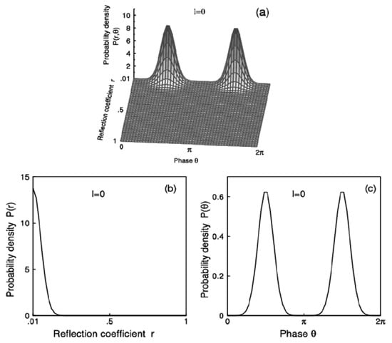
Figure 1.
Initial probability distribution, i.e., when the sample length l = 0: (a) Probability distribution P(r, θ). (b) Marginal reflection probability distribution P(r). (c) Marginal phase probability distribution P(θ).
3. Results
3.1. Evolution of P(r, θ) with the Length L for Different Disorder Strengths
We simulate the evolution of the full probability distribution P(r, θ) for different dimensionless lengths l (=L/ξ) for the three main regimes of disorder strength: (i) weak (2kξ >> 1), (ii) intermediate/medium (2kξ~1), and (iii) strong (2kξ << 1), defined by the disordered strength parameter 2kξ.
3.1.1. P(r, θ) for Weak Disorder: 2kξ = 100 (2kξ >> 1)
Figure 2a–d show typical distributions of the joint probability in (r, θ)-space for different lengths l = 1, 2, 5, and 10. Evolution shows clearly that the phase part is uniformly distributed. Evolution of the probability is mainly along the amplitude (r) axis. Probability evolves with length and peaks near r = 1 for large lengths. These evolution pictures imply that the random (uniform) phase distribution holds for the weak disorder very well, or for the large values of the localization length. Later we show the nearly exact range for the disorder parameter (2kξ) where the random phase approximation is valid for a given length of the sample.
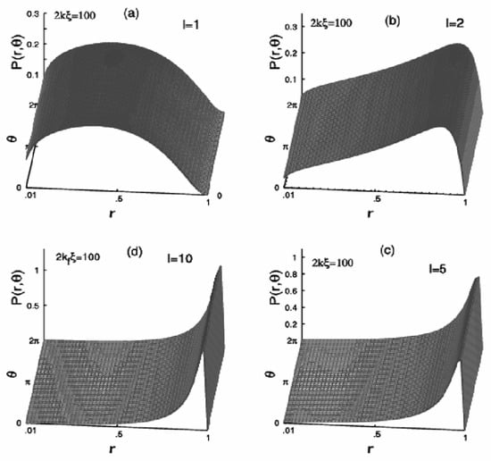
Figure 2.
Evolution of the probability P(r, θ) with the sample length l (=L/ξ) in the weak disorder regime for a fixed disorder strength parameter 2kξ = 100. Plots are for sample lengths: (a) l = 1, (b) l = 2, (c) l = 5, and (d) l = 10.
3.1.2. P(r, θ) for Intermediate/Medium Disorder: 2kξ = 1 (2kξ ~ 1)
Similarly, Figure 3a–d are as Figure 2, but for the disorder strength parameter 2kξ = 1, i.e., medium/intermediate disorder regime. These evolutions clearly show that the probability distribution P(r, θ) is quite complex and has an asymmetric distribution in phase. The phase distribution peaks on one side (2π < θ < π) for large lengths.
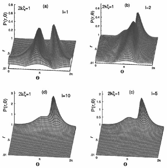
Figure 3.
Evolution of the probability P(r, θ) with the sample length l (=L/ξ) in the medium/intermediate disorder regime for a fixed disorder strength parameter 2kξ = 1. Plots are for sample lengths: (a) l = 1, (b) l = 2, (c) l = 5, and (d) l = 10.
3.1.3. P(r, θ) for Strong Disorder: 2kξ = 0.001 (2kξ << 1)
Similarly, Figure 4a–d are as Figure 2, but for the disorder parameter 2kξ = 0.001, i.e., the strong disorder regime. Probability distribution is perfectly symmetric, centered at the phase θ = π. In the strong disorder parameter regime, the sample tries to behave as a nearly perfect reflector and totally reflect back the incoming wave with opposite phase. Evolution pictures show that P(r, θ) peaks around r = 1 and is symmetrically around θ = π for larger lengths. It will be shown later that the distribution does not change substantially with further increase of the disorder strength parameter, i.e., the distribution is insensitive to the disorder parameter 2kξ in that regime.
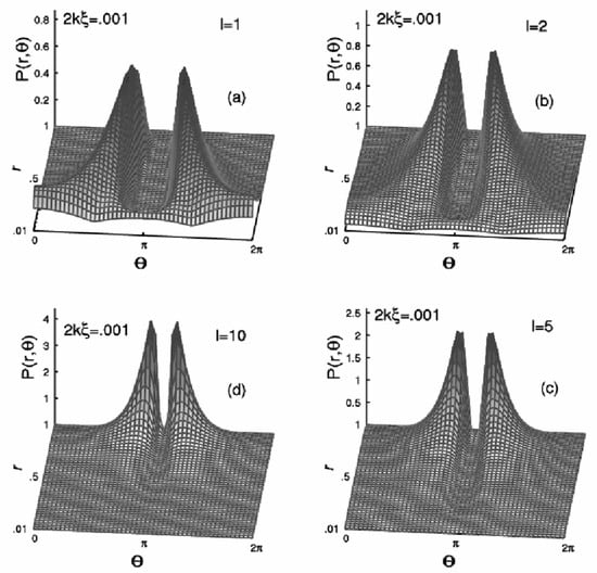
Figure 4.
Evolution of the probability P(r, θ) with the sample length l (=L/ξ) in the strong disorder regime for a fixed disorder strength parameter 2kξ = 0.001. Plots are for sample lengths (a) l = 1, (b) l = 2, (c) l = 5, and (d) l = 10.
3.2. Marginal Distribution P(r) of the Reflection Coefficient (r) and Marginal Distribution P(θ) of the Phase (θ) for: (a) Weak, (b) Medium/Intermediate, and (c) Strong Disorder Regimes
In Figure 5, (i) subplots Figure 5a–c show the marginal probability distribution P(r) when the phase (θ) part of the P(r, θ) is integrated out, and (ii) subplots.
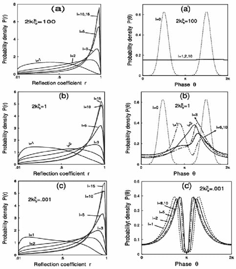
Figure 5.
Marginal probability distribution P(r) for the fixed disorder strength parameters: (a) Weak disorder, 2kξ = 100, (b) Intermediate/medium disorder, 2kξ = 1, and (c) Strong disorder, 2kξ = 0.001 (corresponding to Figure 2, Figure 3 and Figure 4) for different sample lengths. Corresponding marginal phase distributions P(θ) for: (a′) Weak disorder, 2kξ = 100, (b′) Intermediate/medium disorder, 2kξ = 1, and (c′) Strong disorder, 2kξ = 0.001 for the different sample lengths l.
Figure 5a′–c′ are corresponding marginal distributions P(θ) of the phase θ when r part of the full distribution P(r, θ) is integrated out for the three cases of disorder regimes considered above are the (a) weak, (b) medium/intermediate, and (c) strong. Figure 5a′–c′ clearly indicates that the phase (θ) distributions P(θ)s are very different for the three different regimes of disorder parameters considered here. However, as shown in Figure 5a,b, the reflection coefficient (r) distribution does show reasonable variation with the strength of the disorder parameter. Although they are quite different for the smaller length (l~1), they are quite similar for larger lengths (l >> 1). The behavior of the probability distribution indicates that the distribution of the phase has finite effects on the distribution of the reflection coefficient P(r), depending on the length and disorder strength, hence on the average transport properties.
3.3. Distribution of the Phase (θ) with the Strength of Disorder Parameter 2kξ
We now simulate the phase distribution P(θ) with the strength of the disorder parameter (2kξ). We consider here mainly two cases of fixed lengths: (1) l = 1, and (2) the asymptotic limit when l → ∞.
3.3.1. The Phase (θ) Distribution P(θ) for Different Disorder Strength Parameters (2kξ) for Fixed Length l = 1: RPA Regime
Figure 6 shows the plot of P(θ) for the fixed length l = 1, with different values of the disorder strength parameters (2kξ). Figures show that in the strong as well as in the weak disorder limit, P(θ) is insensitive to the strength of the disorder parameter 2kξ, when the length is l~1 or more. In particular, the phase distribution is uniform for the weak disorder case, and it has a perfectly symmetric peak centered at θ = π for the strong disorder case. In the case of intermediate disorder, the distributions are asymmetric with respect to the θ = π point. For the medium/intermediated disorder strength parameter, P(θ) interpolates continuously between the strong and the weak disorder limiting phase distributions.
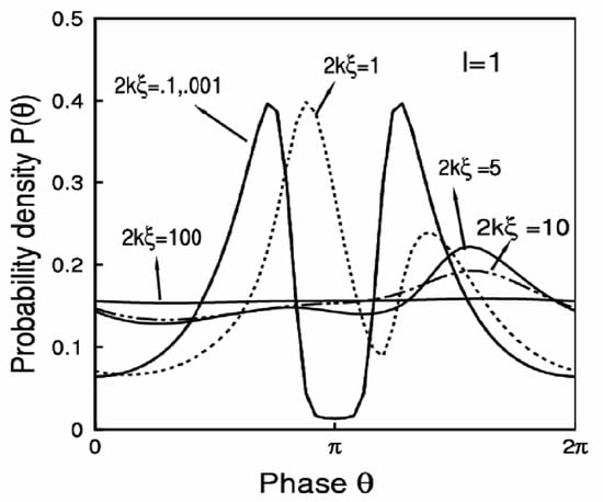
Figure 6.
Phase θ distribution P(θ) against the disorder parameter 2kξ for a fixed sample length l = 1.
RPA validation range: It is clear from the P(θ) distributions, that the random phase approximation (RPA) is valid for the condition ξ > λ = 2π/k, where λ is the wave length of the incoming wave and ξ is the localization length. This has been checked systematically in our numerical calculations. When 2kξ~10, the P(θ) distribution is already deviating from RPA.
3.3.2. The Phase (θ) Distribution P(θ) in the Asymptotic Limit of Large Lengths L→α
Solution of the FP equation (Equation (12)) gives the full probability distribution P(r, θ) in the (r, θ)-space. For larger lengths, one can make the approximation: r ≈ 1 and P(r) ≈ δ(r − 1). In this asymptotic limit, marginal distribution for phase P(θ) becomes:
Now from Equations (11) and (20), we get the marginal probability distribution of phase for larger length limit as:
Figure 7 shows the plot of P(θ) in the asymptotic limit for different disorder strength parameters (2kξ), as the parameter varies from the weak to the strong disorder limits.
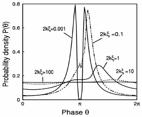
Figure 7.
Phase θ distribution P(θ) against the disorder parameter 2kξ for the asymptotic limit of large length l = 10 (large).
Plots in Figure 7, for large length (i.e., r ≈ 1), show that in the interval from 0 to 2π, (i) a uniform phase distribution in the weak disorder regime; (ii) an asymmetric phase distribution in the intermediate disorder regime; and (iii) a symmetric double peaked distribution around π in the strong disorder regime. These distributions indicate that the essential features of P(θ) have not changed with the r ≈ 1 approximation, relative to the l = 1 case which is shown in Figure 6.
4. Discussion
Numerical simulations show the random phase approximation (RPA) is valid for localization length very much larger than the wavelength, i.e., ξ > λ. Physical meaning of the RPA with this condition is that the incoming wave has to undergo multiple sub-reflections before escaping a localization length and in the process the wave randomizes its phase. This weak disorder regime also can be expressed for a short sample length or within the Born single scattering approximation or regime. For the weak disorder case, the localization length is larger than the wavelength. Hence the phase of the wave gets randomized. In the other extreme case of the strong disorder, the system tries to behave as a perfect reflector. Hence, the phase of the reflected wave tries to peak at π (opposite phase with respect to the incoming wave). In the regime of intermediate disorder, P(θ) distribution is disorder-specific and has some bias points to peak at θ > π. The value of the peaking point of the θ distribution at θ > π can be interpreted as that mostly uniform distributions, however, waves are less back-reflected, rather than penetrating deep before the reflection as the distribution is peaked above θ > π.
At this point we will discuss the results that have been previously reported in the literature. Phase distribution for 1D systems has been studied earlier by Sulem [], Stone et al. [], Jayannavar [], Heinrichs [], and Manna et al. []. Sulem’s result missed the random phase distribution in the limit of weak disorder, however, the calculated phase distributions show peaks near ±π, and it does not show a symmetric distribution as in the present work. The study of Stone et al. showed for the 1D Anderson model that (i) for the case of weak disorder the phase distribution is uniform, (ii) non-uniform for the strong disorder, (iii) and pinning of phase distribution near 2π for very strong disorder and large lengths. Their work also confirms that the distribution of the phase is insensitive to the disorder strength in the limit of weak as well as strong disorder limits. Manna et al. show uniform phase distribution from 0 to 2π for the weak disorder, peaking of the phase distribution near π for the strong disorder, agreeing with the present work. Jayannavar’s calculation for the asymptotic large length (i.e., l → ∞) phase distribution shows a uniform distribution of phase for weak disorder. However, the phase distribution for strong disorder shows several peaks that do not agree with our results.
Marginal Probability Distribution, P(r), of the Reflection Coefficient, r, with Respect to the Disorder Strength Parameter 2kξ
Figure 8 shows the probability distribution, P(r), of the reflection coefficient, r, with the disorder parameter strength (2kξ) for the sample length l = 1. The distributions show weak but finite dependence on the strength of the disorder parameter. The distribution certainly has a small spread, not drastic. It can be seen that though the phase (θ) distribution P(θ) is quite different for different strengths of the disorder parameter (2kξ), the reflection coefficient (r) distribution P(r) does not change drastically with the disorder strength for a fixed length of the sample. However, there is a finite effect of phase on reflection statistics.
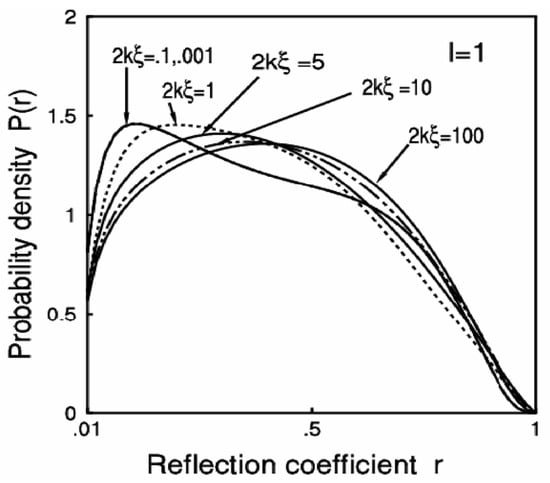
Figure 8.
Reflection coefficient r distribution P(r) against the disorder parameter 2kξ for a fixed sample length l = 1.
5. Conclusions
5.1. Summary of the Phase Distribution Results
We have solved here the 1D optical transport problem for the case of Gaussian white-noise optical disordered potential numerically, by solving joint probability distributions. This is almost a complete solution of transport properties of the 1D Gaussian white-noise random potential that goes beyond the conventional random phase approximation (RPA), or uniform phase distribution, valid only for weak disorder. We have evolved the full probability distribution in the reflection coefficient (r) and the associated phase (θ) space (i.e., (r, θ)-space) of the complex reflection amplitude for a 1D disordered sample, with different lengths and with different disorder strengths. For our numerical solution, we have taken a fixed initial reflection coefficient r0 = 0.01 for all realization of disorder as the Fokker–Planck equation for P(r, θ) is singular at r = 0. Gross statistical properties of the system are not expected to change with this weak extra scatterer. It may, however, affect the very sensitive details corresponding to the limit r → 0 at l → 0. Our numerical work is a systematic study to observe the contribution of the phase fluctuations to reflection coefficient averages.
On the basis of the results obtained, our conclusions are the following:
- Phase θ Distribution P(θ) in Different Regimes of Disorder:
(1). The random phase approximation (RPA) implying uniform phase distribution over 2π is valid for the condition ξ/λ >> 1 (ξ is the localization length and λ is incoming wavelength), that is, in the weak disorder limit. Physically, this means that the wave has to undergo multiple sub-reflections before it moves through one localization length or scattering mean free path. P(θ) is independent of the disorder in the weak disorder limit (2kξ >> 1).
(2). In the intermediate disorder regime, phase distribution is complex and asymmetric, about θ = π point in the interval 0 and 2π, peaking in between π and 2π. In addition, the phase distributions are strongly disordered strength parameters, 2kξ, dependent. In this regime back-reflection is less prominent than the uniform distribution, however, the wave is back-reflected after a deep penetration. This provides us with an understanding of the peak of the reflected wave around 2π.
(3). In the strong disorder regime, the distribution of the phase is perfectly symmetric in the interval from 0 and 2π, centering at θ = π. This arises due to the opposite phase of the back reflected wave in the disordered regime. The distribution is independent of the disorder in the strong disorder limit (2kξ << 1) even for smaller sample lengths.
5.2. Reflection Coefficient (r) Distributions P(r)
The probability distribution for the reflection coefficient peaks at r = 1 for large lengths l ≡ L/ξ >> 1. Though probability distribution P(θ) for the phase varies largely with the variation of the disorder strength, the probability distribution for the reflection coefficient P(r) does not change drastically with the disorder strength for a fixed length of the sample. In particular, phase distribution has weaker but finite effects on the reflection coefficient distribution.
5.3. Extension of the Phase Distribution to Electronic Case
For 1D, the Schrödinger and the Maxwell equations project to the Helmholtz equation, and they are similar to each other, only the form of the potentials are different. The Landauer four-probe resistance formula [] shows that the dimensionless resistance as a function of the reflection coefficient:
Making the transformation from P(r) to P(ρ) by using P(ρ) = P(r)(dr/dρ), one obtains the Fokker–Planck equation for the resistance, and the mean and the STD of the resistance can be derived from the above variable change as shown in detail in []. The functional change in the magnitude of the reflection will not change the form of the value of the phase distribution, therefore, the phase distribution of the resistance will be the same as the phase distribution of the reflection coefficient.
5.4. Applications of the Phase Statistics
1D disordered media is equivalent to the continuum of the discrete random layered media. These types of media appear in optical media in semiconductors, layered electronic media, atmospheric dielectric layered media for different electromagnetic wave transportation through our atmosphere, underground dielectric layered media in search of earth’s underground oils. The reflection is associated with phase, therefore it is important to know the actual phase distribution to better predict the regime of the reflection. In addition, 1D disordered media may be used for the phase randomizer for electrical or electronics cases. Recently 1D disordered media is used for one-dimensional multi-channel analysis of the light reflected from biological cells for ultra-early cancer detection [,], as well as transport in stochastic absorbing media []. Knowing 1D phase distribution would be helpful for accurate parameterization of the reflection coefficients as well as understanding the random layered media.
Other applications of PF approach in electromagnetic waves: PF approach has been applied for studying optical memory effect [] and also for paraxial imaging using X-ray [].
Funding
National Institute of Health (Grant No. R21CA260147) and Mississippi State University.
Institutional Review Board Statement
Not applicable.
Informed Consent Statement
Not applicable.
Data Availability Statement
Available from the authour on request.
Acknowledgments
The author gratefully acknowledges N. Kumar for stimulating discussions. The work was partially supported by the National Institute of Health (Grant No. R21CA260147) and Mississippi State University.
Conflicts of Interest
The author declares that there is no conflict of interest regarding the publication of this article.
References
- Mott, N.F.; Twose, W.D. The theory of impurity conduction. Adv. Phys. 1961, 10, 107. [Google Scholar] [CrossRef]
- Mott, N.F. Electrons in disordered structures. Adv. Phys. 1967, 16, 49. [Google Scholar] [CrossRef]
- Ishii, K. Localization of eigenstates and transport phenomena in one-dimensional disordered systems. Prog. Theor. Phys. Suppl. 1973, 53, 77. [Google Scholar] [CrossRef]
- Thouless, J.D. Electrons in disordered systems and the theory of localization. Phys. Rep. 1974, 13, 93. [Google Scholar] [CrossRef]
- Abrikosov, A.A.; Ryzhkin, I.A. Conductivity of quasi-one-dimensional metal systems. Adv. Phys. 1977, 27, 147. [Google Scholar] [CrossRef]
- Erdös, P.; Herndon, R.C. Theories of electrons in one-dimensional disordered systems. Adv. Phys. 1982, 31, 65. [Google Scholar] [CrossRef]
- Lee, P.A.; Ramakrishnan, T.V. Disordered electronic systems. Rev. Mod. Phys. 1985, 57, 287. [Google Scholar] [CrossRef]
- Papanicolaou, G.C. Wave propagation in a one-dimensional random medium. SIAM J. Appl. Math. 1971, 21, 13. [Google Scholar] [CrossRef][Green Version]
- Frisch, U.; Gautero, J.L. Backscattering and localization of high-frequency waves in a onedimensional random medium. J. Math. Phys. 1984, 25, 1378. [Google Scholar] [CrossRef]
- Kumar, N. Resistance fluctuation in a one-dimensional conductor with static disorder. Phys. Rev. B 1985, 31, 5513. [Google Scholar] [CrossRef]
- Heinrichs, J. Invariant-imbedding approach to resistance fluctuations in disordered one-dimensional conductors. Phys. Rev. 1986, 33, 2561. [Google Scholar] [CrossRef] [PubMed]
- Rammal, R.; Doucot, B. Invariant imbedding approach to localization. I. General framework and basic equations. J. Phys. 1987, 48, 509. [Google Scholar] [CrossRef]
- Pradhan, P.; Kumar, N. Localization of light in coherently amplifying random media. Phys. Rev. B 1994, 50, 9644. [Google Scholar] [CrossRef] [PubMed]
- Pradhan, P. A model for quantum stochastic absorption in absorbing disordered media. Phys. Rev. B 2006, 74, 085107. [Google Scholar] [CrossRef]
- Azbel, M.Y. Eigenstates and properties of random systems in one dimension at zero temperature. Phys. Rev. B 1983, 28, 4106. [Google Scholar] [CrossRef]
- Melnikov, V.I. Fluctuations in the resistivity of a finite disordered system. Sov. Phys. Solid State 1981, 23, 444. [Google Scholar]
- Van Kampen, N.G. Stochastic differential equations. Phys. Rep. 1976, 24, 172. [Google Scholar] [CrossRef]
- Novikov, A.E. Functionals and the Random-force Method in Turbulence Theory. Sov. Phy. JETP 1965, 20, 1290. [Google Scholar]
- Mello, P.A.; Kumar, N. Information theory and one-dimensional disordered conductors. J. Non-Cryst. Solids 1985, 75, 135. [Google Scholar] [CrossRef]
- Press, W.H.; Teukolsky, S.A.; Vetterling, W.T.; Flannery, B.P. Numerical Recipies; Cambridge University Press: Cambridge, UK, 1986. [Google Scholar]
- Ames, W.F. Numerical Methods for Partial Differential Equations; Academic Press: New York, NY, USA, 1977. [Google Scholar]
- Sulem, P.L. Total reflection of a plane wave from a semi-infinite, one-dimensional random medium: Distribution of the phase. Physica 1973, 70, 190. [Google Scholar] [CrossRef]
- Stone, A.D.; Allan, D.C.; Joannopoulos, J.D. Phase randomness in the one-dimensional Anderson model. Phys. Rev. B 1983, 27, 836. [Google Scholar] [CrossRef]
- Jayannavar, M. Scaling theory of quantum resistance distributions in disordered systems. Pramana J. Phys. 1991, 36, 611. [Google Scholar] [CrossRef]
- Heinrichs, J. Phase-shift randomness in one-dimensional disordered conductors in the quasi-metallic domain. J. Phys. C Solid State Phys. 1988, 21, L1153. [Google Scholar] [CrossRef]
- Manna, S.K.; Mukherjee, A. Numerical Study of the distribution of phase as an electron moves in a one-dimensional continuously and randomly varying potential. Int. Jr. Mod. Phys. B 1992, 6, 1517. [Google Scholar] [CrossRef]
- Landauer, R. Electrical resistance of disordered one-dimensional lattices. Phylos. Mag. 1970, 21, 863. [Google Scholar] [CrossRef]
- Subramanian, H.; Pradhan, P.; Liu, Y.; Capoglu, I.R.; Rogers, J.D.; Roy, H.K.; Brand, R.E.; Backman, V. Partial wave microscopic spectroscopy detects sub-wavelength refractive index fluctuations: An application to cancer diagnosis. Opt. Lett. 2009, 34, 518–520. [Google Scholar] [CrossRef] [PubMed]
- Subramanian, H.; Pradhan, P.; Liu, Y.; Capoglu, I.R.; Li, X.; Rogers, J.D.; Heifetz, A.; Kunte, D.; Roy, H.K.; Taflove, A.; et al. Optical methodology for detecting histologically unapparent nanoscale consequences of genetic alterations in biological cells. Proc. Nat. Acad. Sci. USA 2008, 150, 20124. [Google Scholar] [CrossRef]
- Osnabrugge, G.; Horstmeyer, R.; Papadopoulos, I.N.; Judkewitz, B.; Vellekoop, I.M. Generalized optical memory effect. Optica 2017, 4, 886–892. [Google Scholar] [CrossRef]
- Paganin, D.M.; Morgan, K.S. X-ray Fokker–Planck equation for paraxial imaging. Sci. Rep. 2019, 9, 17537. [Google Scholar] [CrossRef]
Publisher’s Note: MDPI stays neutral with regard to jurisdictional claims in published maps and institutional affiliations. |
© 2021 by the author. Licensee MDPI, Basel, Switzerland. This article is an open access article distributed under the terms and conditions of the Creative Commons Attribution (CC BY) license (https://creativecommons.org/licenses/by/4.0/).