Wide-Field Telescope Alignment Using the Model-Based Method Combined with the Stochastic Parallel Gradient Descent Algorithm

Abstract
1. Introduction
2. Theory
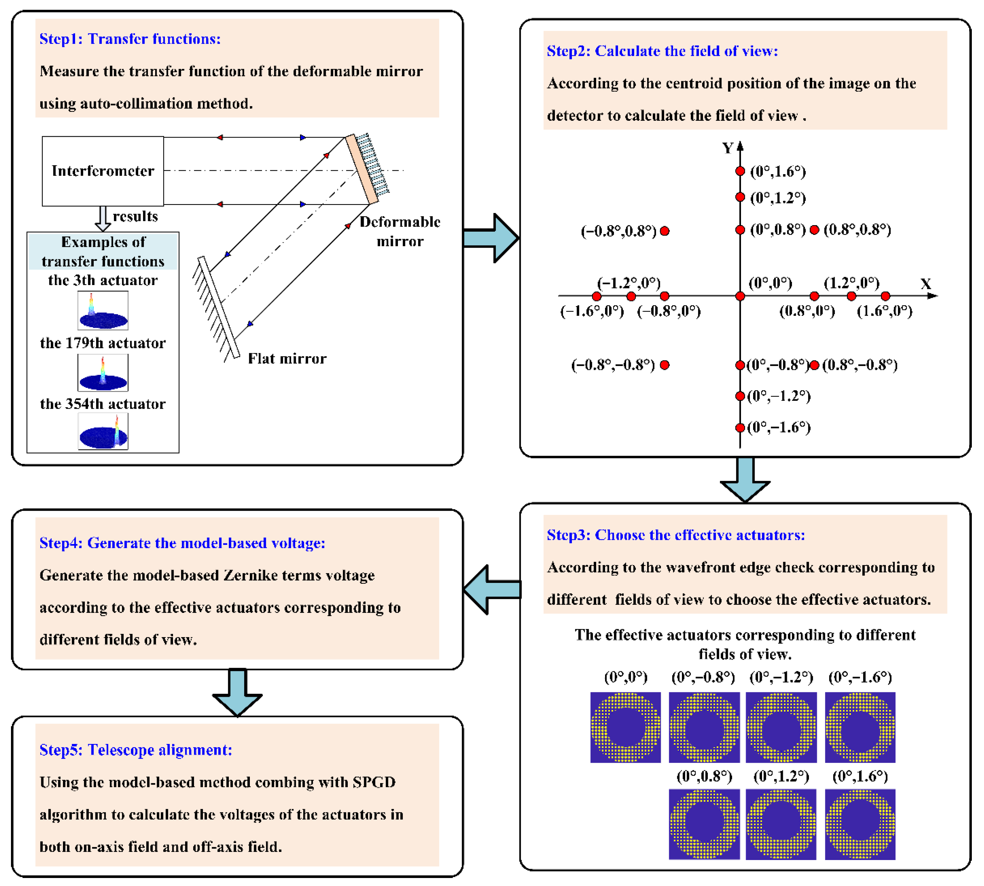
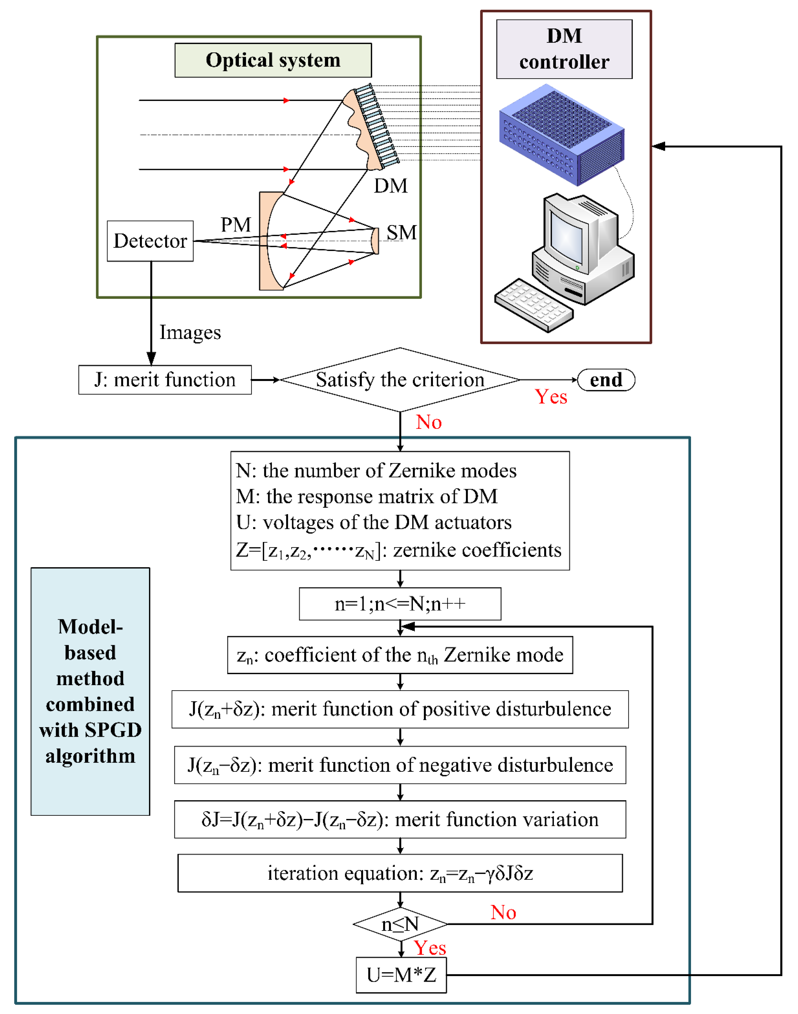
2.1. The Model-Based Method Combined with the SPGD Algorithm
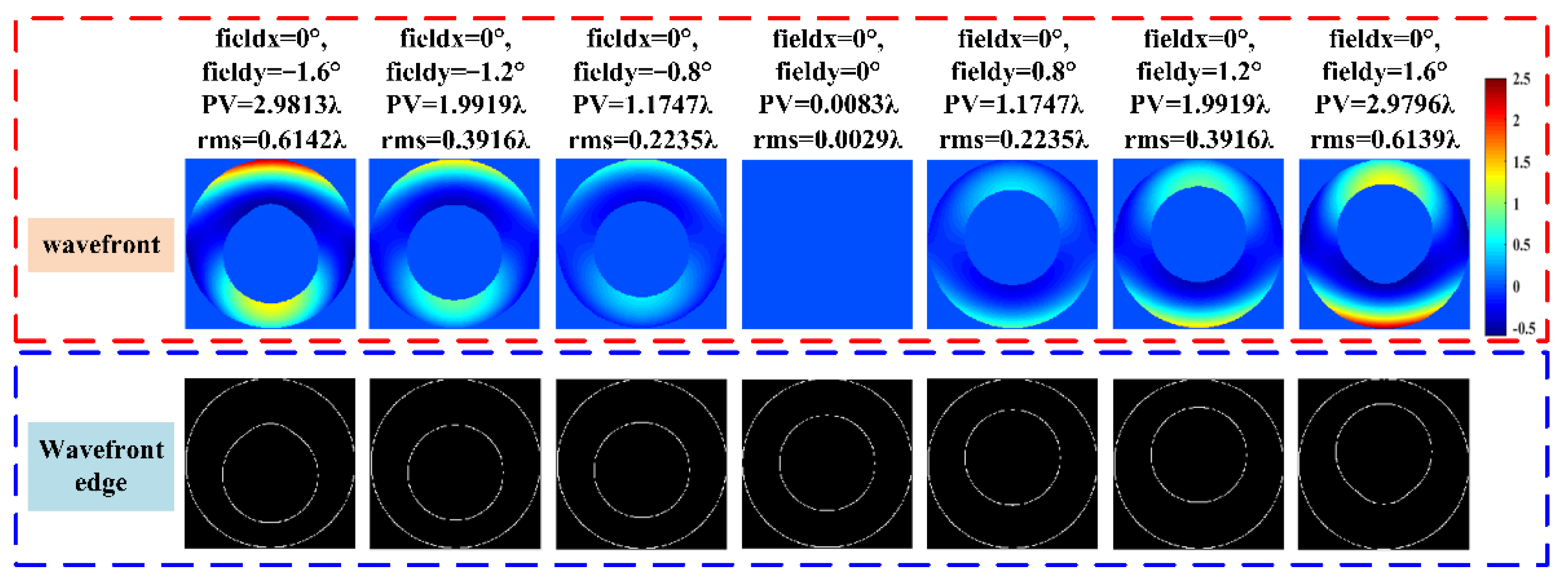
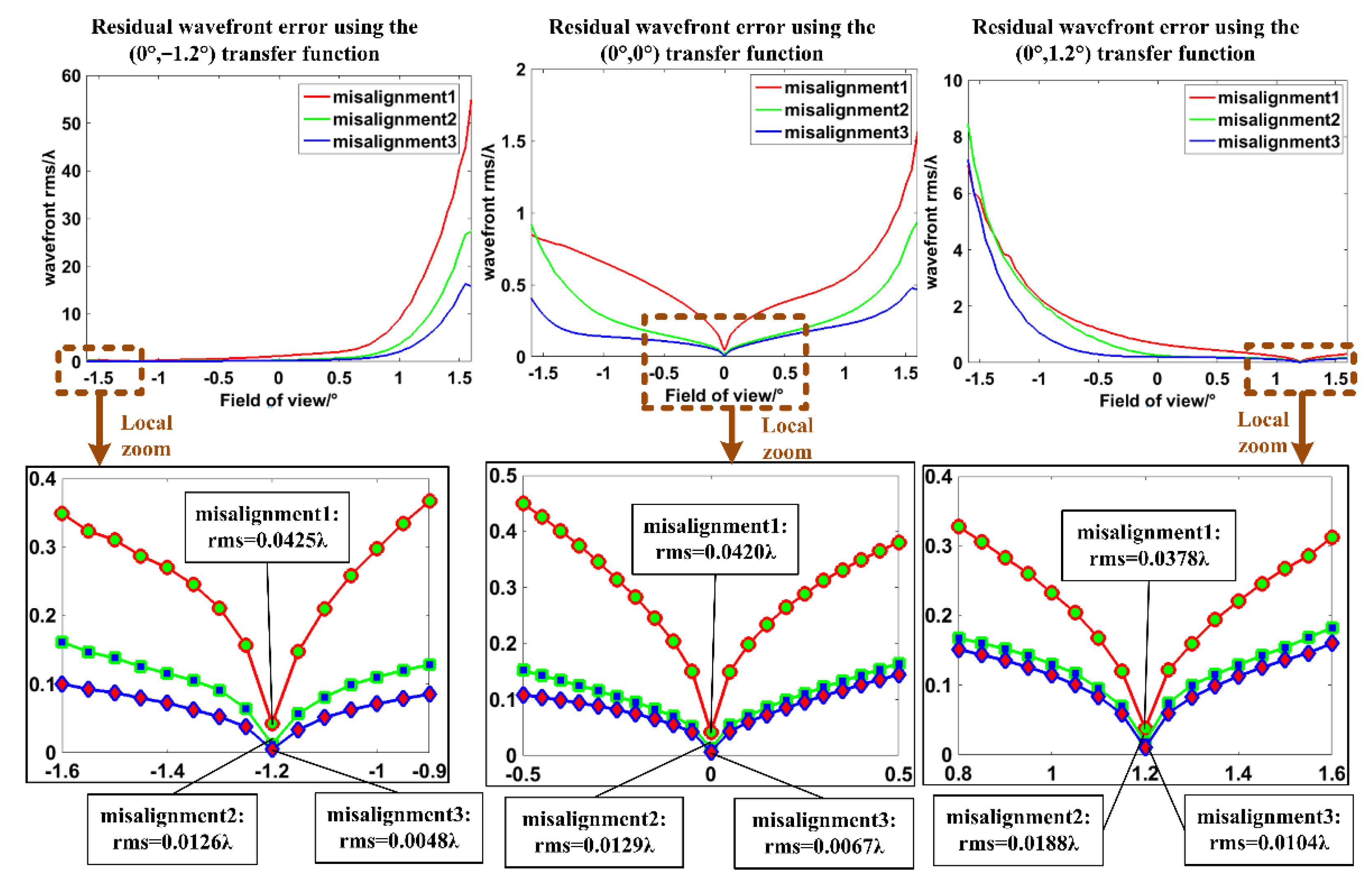
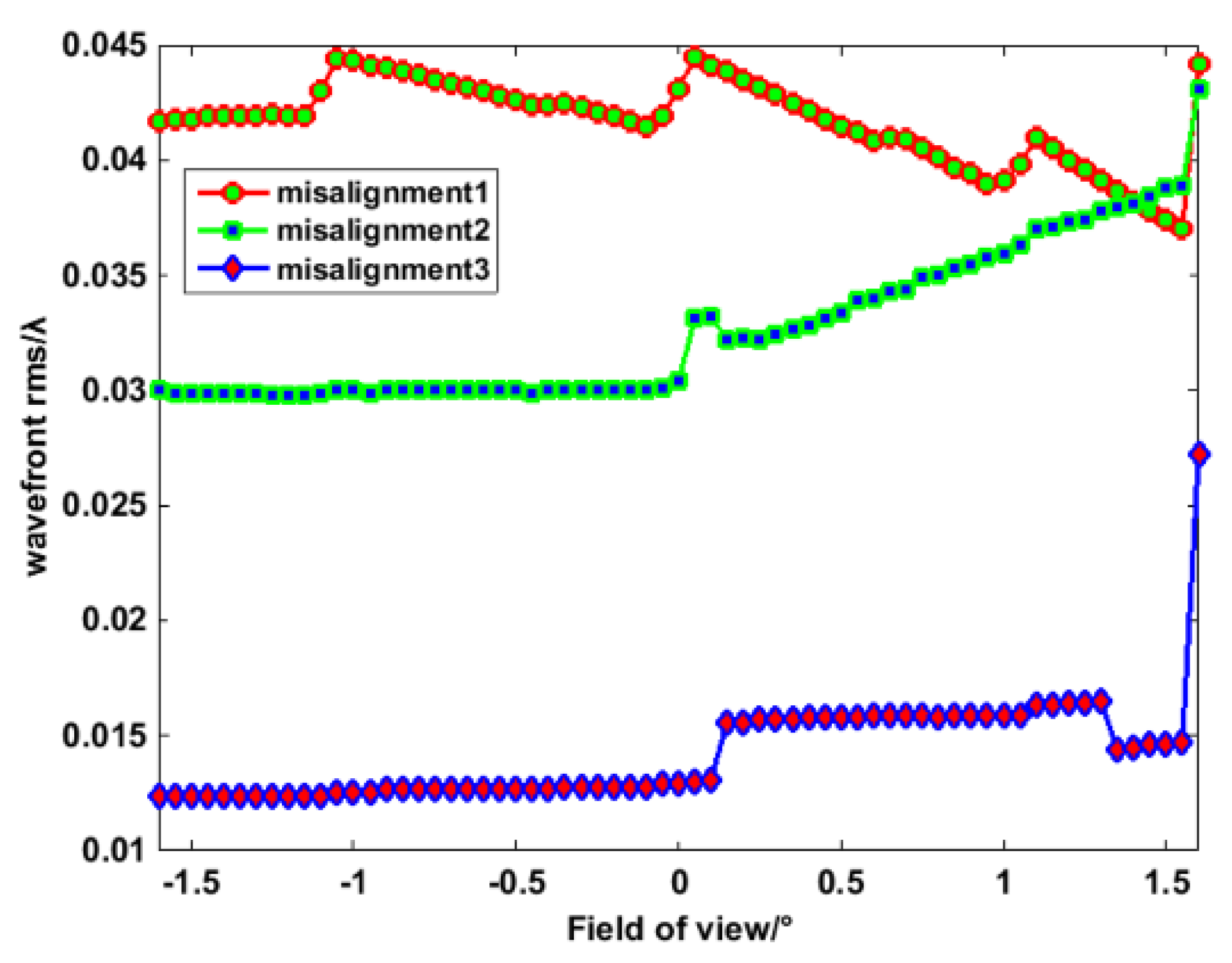
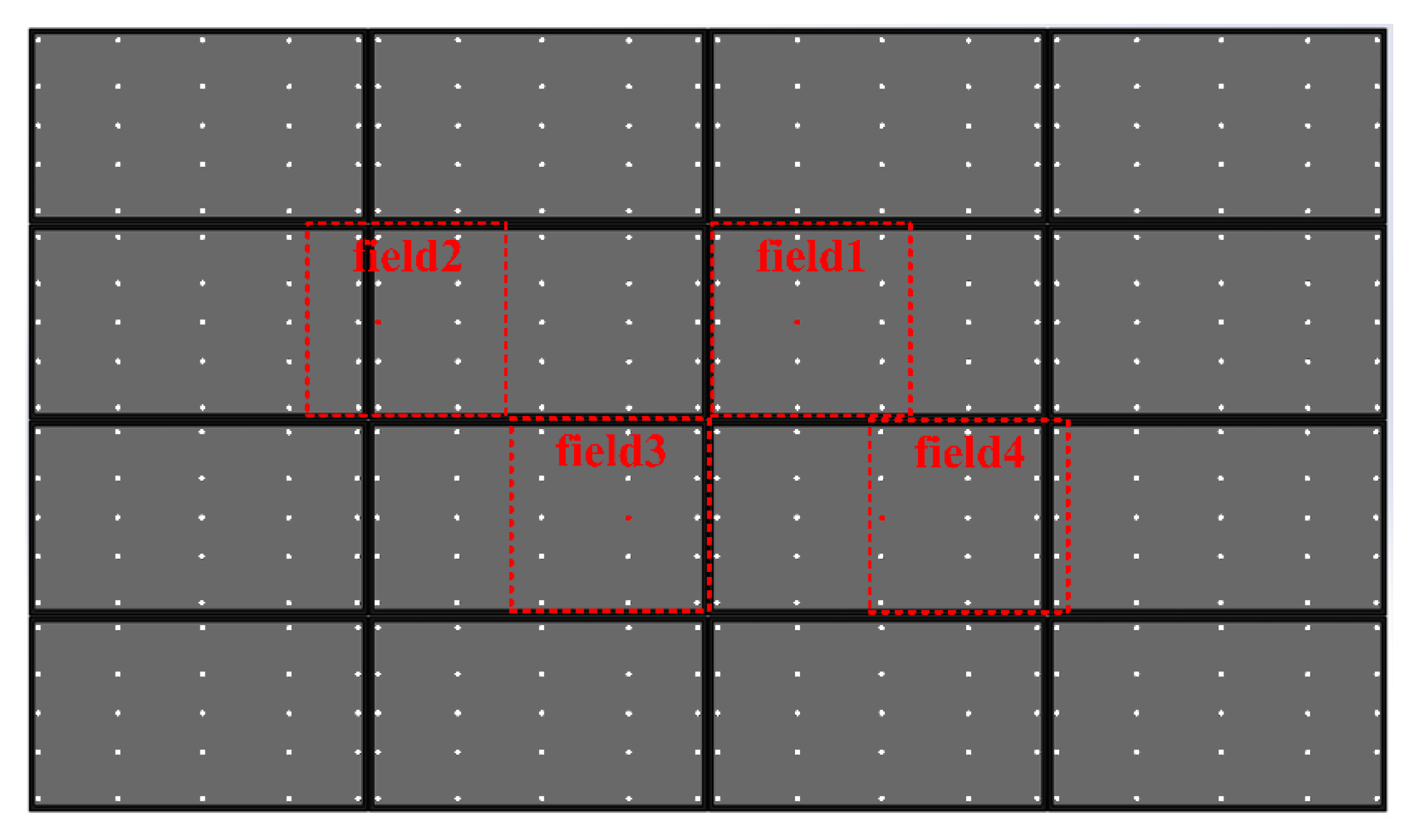
2.2. Transfer Functions of the Deformable Mirror Corresponding to Different Fields of View
3. Experiments
3.1. Experiment System
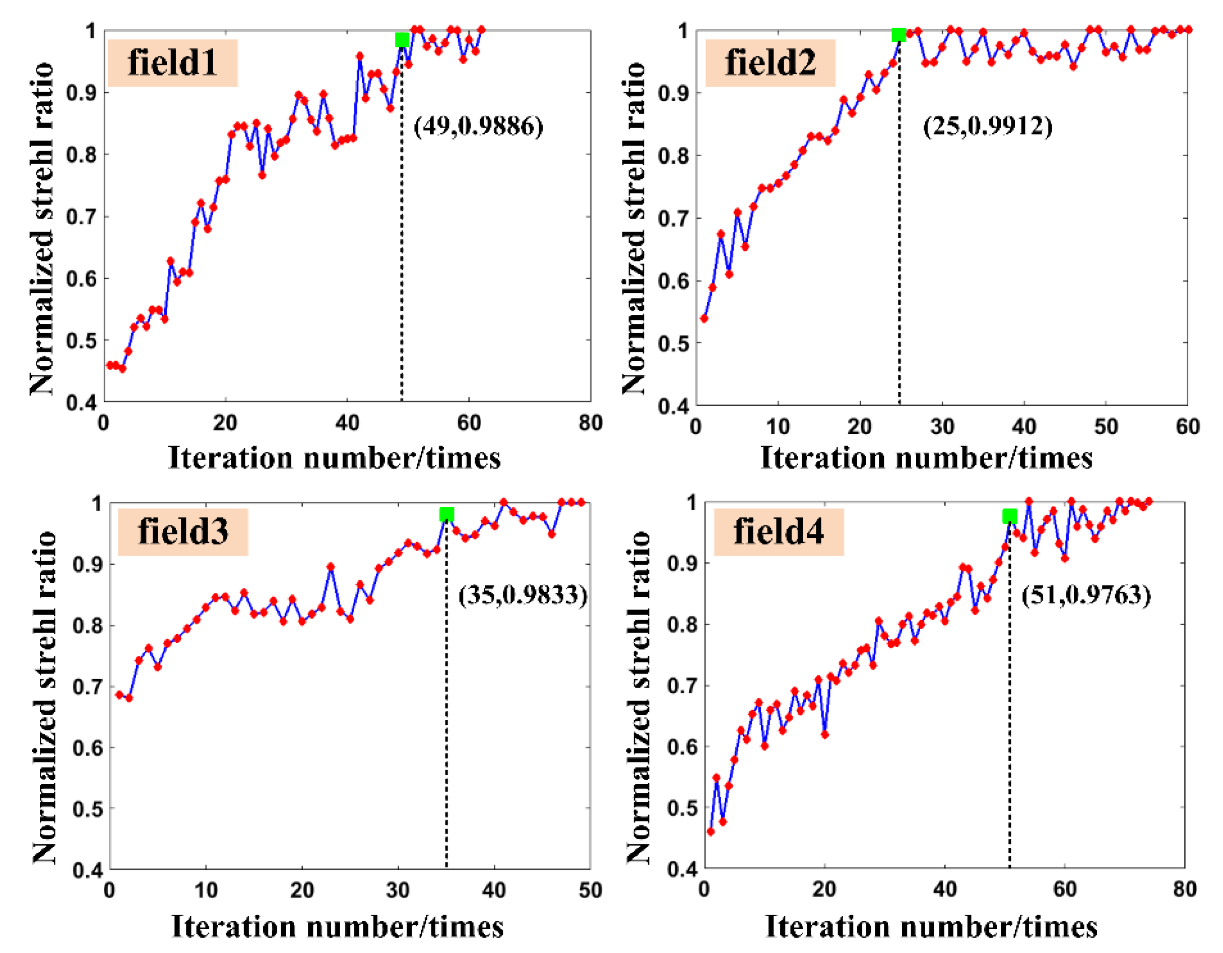
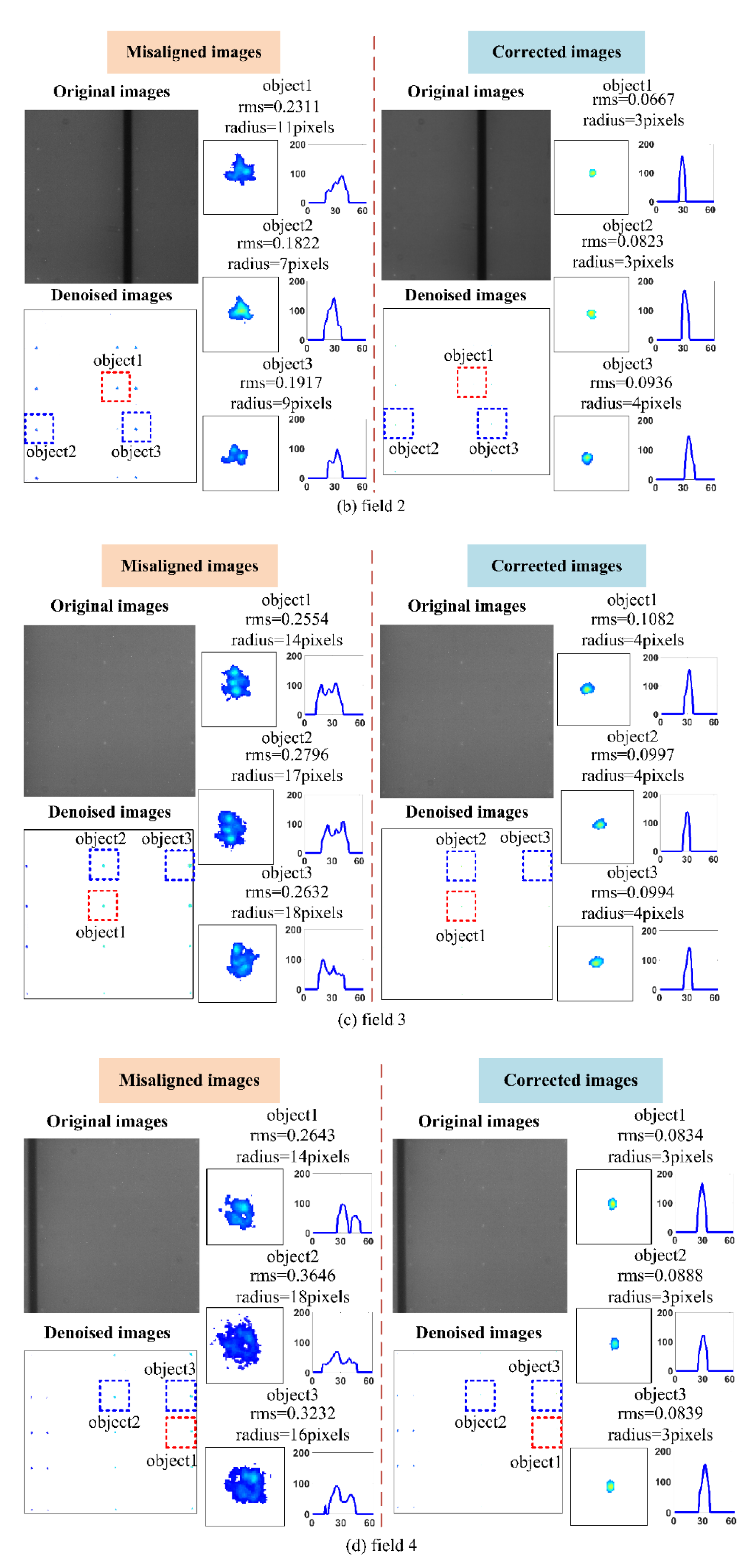
3.2. Experiment Results
4. Conclusions
Author Contributions
Funding
Conflicts of Interest
References
- Lin-Hai, H. Coherent beam combination using a general model-based method. Chin. Phys. Lett. 2014, 31, 094205–094207. [Google Scholar]
- Wang, S.Q.; Wei, K.; Zheng, W.J.; Rao, C.H. First light on an adaptive optics system using a non-modulation pyramid wavefront sensor for a 1.8 m telescope. Chin. Opt. Lett. 2016, 14, 100101–100105. [Google Scholar] [CrossRef]
- Xie, Z.L.; Ma, H.T.; Qi, B.; Ren, G.; Shi, J.; He, X.; Tan, Y.; Dong, L.; Wang, Z. Experimental demonstration of enhanced resolution of a Golay3 sparse-aperture telescope. Chin. Opt. Lett. 2017, 15, 041101–041104. [Google Scholar]
- Bolcar, M.; Fienup, J. Sub-aperture piston phase diversity for segmented and multi-aperture systems. Appl. Opt. 2009, 48, A5–A12. [Google Scholar] [CrossRef]
- Antonello, J.; Verhaegen, M. Modal-based phase retrieval for adaptive optics. J. Opt. Soc. Am. A 2015, 32, 1160–1170. [Google Scholar] [CrossRef]
- Yeh, L.H.; Dong, J.; Zhong, J.; Tian, L.; Chen, M.; Tang, G.; Soltanolkotabi, M.; Waller, L. Experimental robustness of Fourier ptychography phase retrieval algorithms. Opt. Express 2015, 23, 33214–33240. [Google Scholar] [CrossRef] [PubMed]
- Yang, Q.; Zhao, J.; Wang, M.; Jia, J. Wavefront sensorless adaptive optics based on the trust region method. Opt. Lett. 2015, 40, 1235–1237. [Google Scholar] [CrossRef]
- Yang, P.; Ao, M.W.; Liu, Y.; Xu, B.; Jiang, W. Intracavity transverse modes controlled by a genetic algorithm based on zernike mode coefficients. Opt. Express 2007, 15, 17051–17062. [Google Scholar] [CrossRef]
- Conkey, D.B.; Brown, A.N.; Caravaca-Aguirre, A.M.; Piestun, R. Genetic algorithm optimization for focusing through turbid media in noisy environments. Opt. Express 2012, 20, 4840–4849. [Google Scholar] [CrossRef]
- Marsh, P.; Burns, D.; Girkin, J. Practical implementation of adaptive optics in multiphoton microscopy. Opt. Express 2003, 11, 1123–1130. [Google Scholar] [CrossRef] [PubMed]
- Theofanidou, E.; Wilson, L.; Hossack, W.J.; Arlt, J. Spherical aberration correction for optical tweezers. Opt. Commun. 2004, 236, 145–150. [Google Scholar] [CrossRef]
- Zommer, S.; Ribak, E.N.; Lipson, S.G.; Adler, J. Simulated annealing in ocular adaptive optics. Opt. Lett. 2006, 31, 939–941. [Google Scholar] [CrossRef]
- Geng, C.; Luo, W.; Tan, Y.; Liu, H.; Mu, J.; Li, X.Y. Experimental demonstration of using divergence cost function in SPGD algorithm for coherent beam combining with tip/tilt control. Opt. Express 2013, 21, 25045–25055. [Google Scholar] [CrossRef]
- Yang, H.Z.; Zhang, Z.; Wu, J. Performance comparison of wavefront-sensorless adaptive optics systems by using of the focal plane. Int. J. Opt. 2015, 2015, 985351. [Google Scholar] [CrossRef][Green Version]
- Ren, H.X.; Dong, B. Improved model-based wavefront sensorless adaptive optics for extended objects using N + 2 images. Opt. Express 2020, 28, 14414–14427. [Google Scholar] [CrossRef]
- Wen, L.H.; Yang, P.; Yang, K.J.; Chen, S.Q.; Wang, S.; Liu, W.J.; Xu, B. Synchronous model-based approach for wavefront sensorless adaptive optics system. Opt. Express 2017, 25, 20584–20597. [Google Scholar]
- Yang, H.Z.; Soloviev, O.; Verhaegen, M. Model-based wavefront sensorless adaptive optics system for large aberrations and extended objects. Opt. Express 2015, 23, 24587–24601. [Google Scholar] [CrossRef] [PubMed]
- Li, M.; Liu, X.; Zhang, A.; Xian, H. Telescopes alignment using the sharpness function method based on under-sampled images. IEEE PJ 2019, 1, 1–14. [Google Scholar]
- Fu, Q.; Pott, J.; Shen, F.; Rao, C.H.; Li, X.Y. Stochastic parallel gradient descent optimization based on decoupling of the software and hardware. Opt. Commun. 2014, 310, 138–149. [Google Scholar] [CrossRef][Green Version]
- Dong, B.; Yu, J. Hybrid approach used for extended image-based wavefront sensor-less adaptive optics. Opt. Lett. 2015, 4, 041101–041110. [Google Scholar] [CrossRef]
- Dong, B.; Ren, D.Q.; Zhang, X. Stochastic parallel gradient descent based adaptive optics used for a high contrast imaging coronagraph. Res. Astron. Astrophys. 2011, 11, 997–1002. [Google Scholar] [CrossRef]
- Wang, X.L.; Zhou, P.; Ma, Y.X.; Leng, J.Y.; Xu, X.J.; Liu, Z.J. Active phasing a nine-element 1.14 kW all-fiber two-tone MOPA array using SPGD algorithm. Opt. Lett. 2011, 36, 3121–3123. [Google Scholar] [CrossRef]
- Born, M.; Wolf, E. Principles of Optics, 2nd ed.; Cambridge University Press: Cambridge, UK, 1999. [Google Scholar]
- Huang, L.H.; Rao, C.H. Wavefront sensorless adaptive optics: A general model-based approach. Opt. Express 2011, 19, 371–379. [Google Scholar]
- Booth, M.J. Wavefront sensor-less adaptive optics: A model-based approach using sphere packings. Opt. Express 2006, 14, 1339–1352. [Google Scholar] [CrossRef] [PubMed]
- Li, M.; Liu, X.; Zhang, A.; Xian, H. Telescope alignment based on the sharpness function of under-sampled images. Chin. Opt. Lett. 2019, 6, 061101–061105. [Google Scholar] [CrossRef]


| Field | cxout/mm | cyout/mm | cxin/mm | cyin/mm | Standard Deviation/mm |
|---|---|---|---|---|---|
| (0°, −1.6°) | 18.58 | 18.47 | 18.58 | 20.88 | 2.41 |
| (0°, −1.2°) | 18.58 | 18.47 | 18.58 | 20.42 | 1.95 |
| (0°, −0.8°) | 18.58 | 18.47 | 18.58 | 19.77 | 1.30 |
| (0°, 0°) | 18.58 | 18.47 | 18.58 | 18.45 | 0.02 |
| (0°, 0.8°) | 18.58 | 18.47 | 18.58 | 17.13 | 1.34 |
| (0°, 1.2°) | 18.58 | 18.47 | 18.58 | 16.48 | 1.99 |
| (0°, 1.6°) | 18.58 | 18.47 | 18.58 | 16.09 | 2.38 |
| Zernike Order | Z4/λ | Z5/λ | Z6/λ | Z7/λ | Z8/λ | Z11/λ |
|---|---|---|---|---|---|---|
| Misalignment 1 | 1 | 1 | −1 | −1 | 1 | 1 |
| Misalignment 2 | 0.3 | −0.2 | 0.8 | 0.1 | −0.6 | −0.5 |
| Misalignment 3 | −0.1 | 0.4 | −0.5 | 0.2 | 0.3 | −0.2 |
| RMS | ||||||
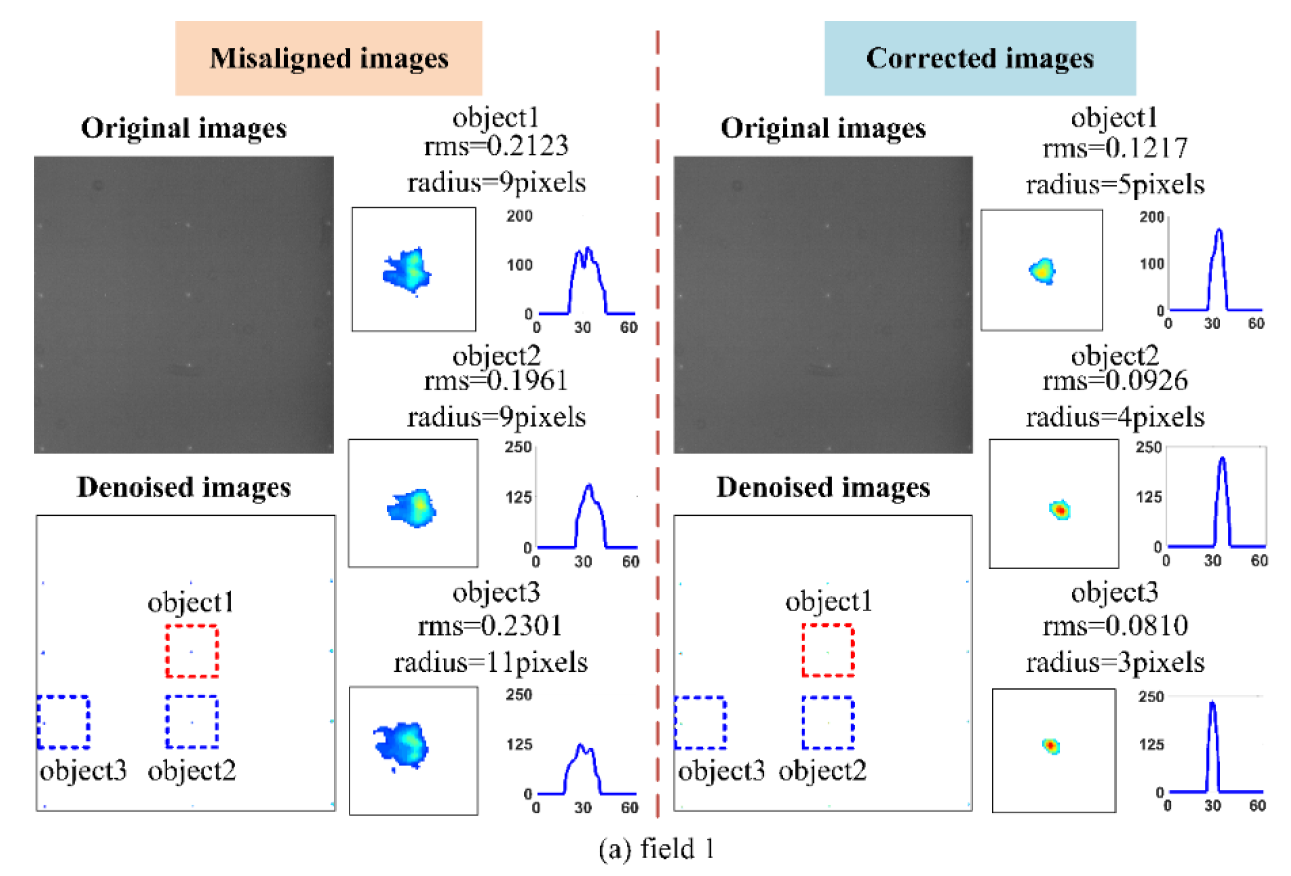
| Field | Object 1 | Object 2 | Object 3 | |||
| Misaligned Images | Corrected Images | Misaligned Images | Corrected Images | Misaligned Images | Corrected Images | |
| 1 | 0.2123 | 0.1217 | 0.1961 | 0.0926 | 0.2301 | 0.0810 |
| 2 | 0.2311 | 0.0667 | 0.1822 | 0.0823 | 0.1917 | 0.0936 |
| 3 | 0.2554 | 0.1082 | 0.2796 | 0.0997 | 0.2632 | 0.0994 |
| 4 | 0.2643 | 0.0834 | 0.3646 | 0.0888 | 0.3232 | 0.0839 |
| Radius/pixels | ||||||
| Field | Object 1 | Object 2 | Object 3 | |||
| Misaligned Images | Corrected Images | Misaligned Images | Corrected Images | Misaligned Images | Corrected Images | |
| 1 | 9 | 5 | 9 | 4 | 11 | 3 |
| 2 | 11 | 3 | 7 | 3 | 9 | 4 |
| 3 | 14 | 4 | 17 | 4 | 18 | 4 |
| 4 | 14 | 3 | 18 | 3 | 16 | 3 |
Publisher’s Note: MDPI stays neutral with regard to jurisdictional claims in published maps and institutional affiliations. |
© 2021 by the authors. Licensee MDPI, Basel, Switzerland. This article is an open access article distributed under the terms and conditions of the Creative Commons Attribution (CC BY) license (https://creativecommons.org/licenses/by/4.0/).
Share and Cite
Li, M.; Zhang, A.; Zhang, J.; Xian, H. Wide-Field Telescope Alignment Using the Model-Based Method Combined with the Stochastic Parallel Gradient Descent Algorithm. Photonics 2021, 8, 463. https://doi.org/10.3390/photonics8110463
Li M, Zhang A, Zhang J, Xian H. Wide-Field Telescope Alignment Using the Model-Based Method Combined with the Stochastic Parallel Gradient Descent Algorithm. Photonics. 2021; 8(11):463. https://doi.org/10.3390/photonics8110463
Chicago/Turabian StyleLi, Min, Ang Zhang, Junbo Zhang, and Hao Xian. 2021. "Wide-Field Telescope Alignment Using the Model-Based Method Combined with the Stochastic Parallel Gradient Descent Algorithm" Photonics 8, no. 11: 463. https://doi.org/10.3390/photonics8110463
APA StyleLi, M., Zhang, A., Zhang, J., & Xian, H. (2021). Wide-Field Telescope Alignment Using the Model-Based Method Combined with the Stochastic Parallel Gradient Descent Algorithm. Photonics, 8(11), 463. https://doi.org/10.3390/photonics8110463