Dual-Modality Imaging Microfluidic Cytometer for Onsite Detection of Phytoplankton


Abstract
:1. Introduction
2. Materials and Methods
2.1. Materials
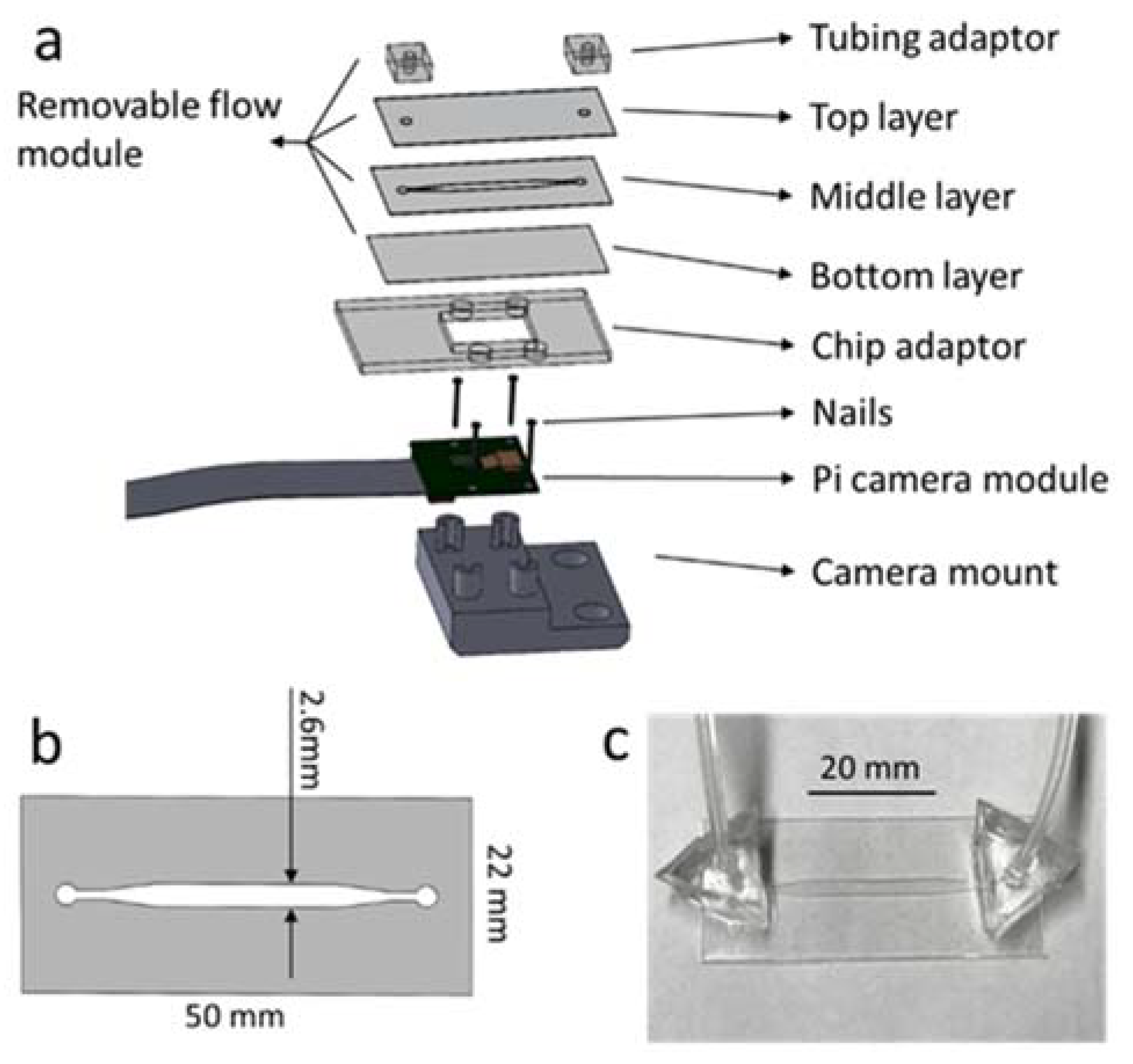
2.2. System Design
2.3. Microfluidic Chip Design
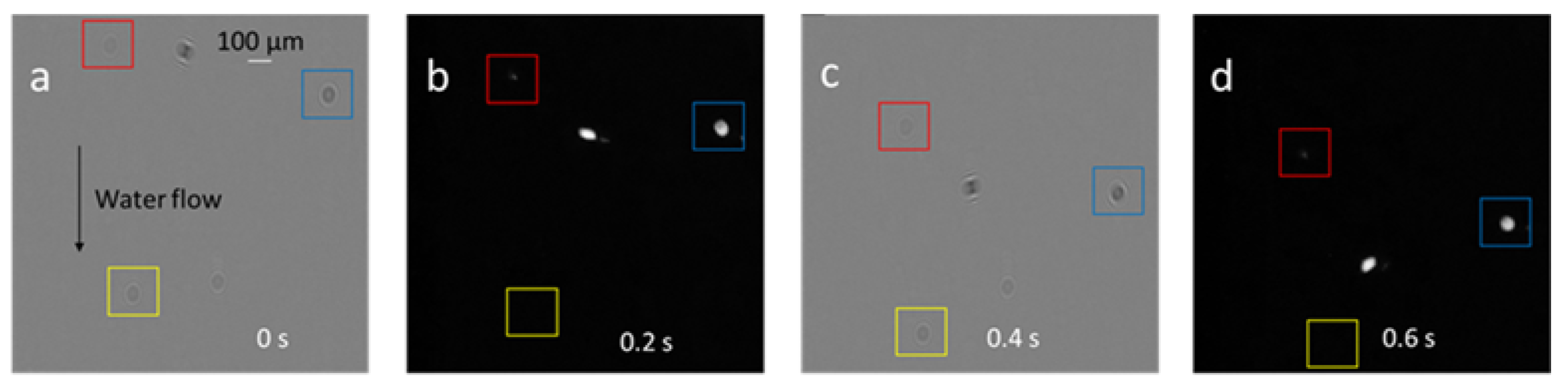
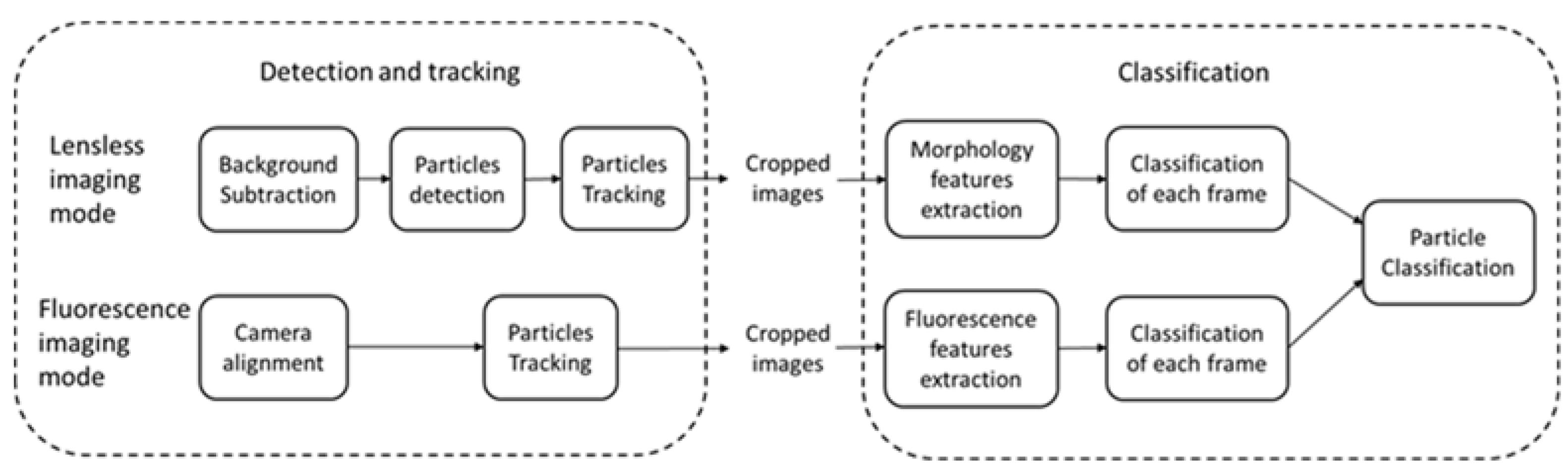
2.4. Image Processing Algorithms
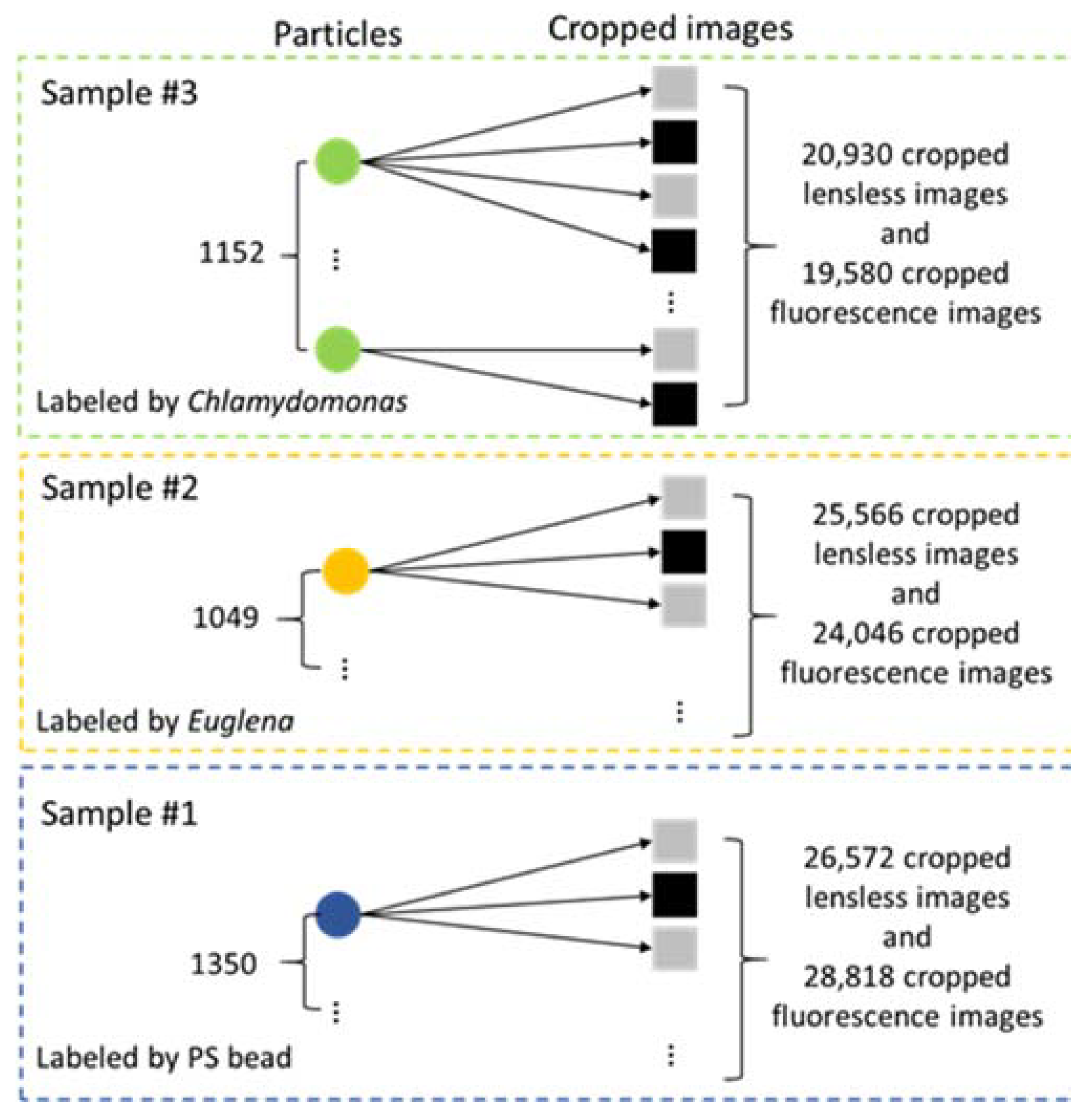
2.5. Sample Preparation
3. Results
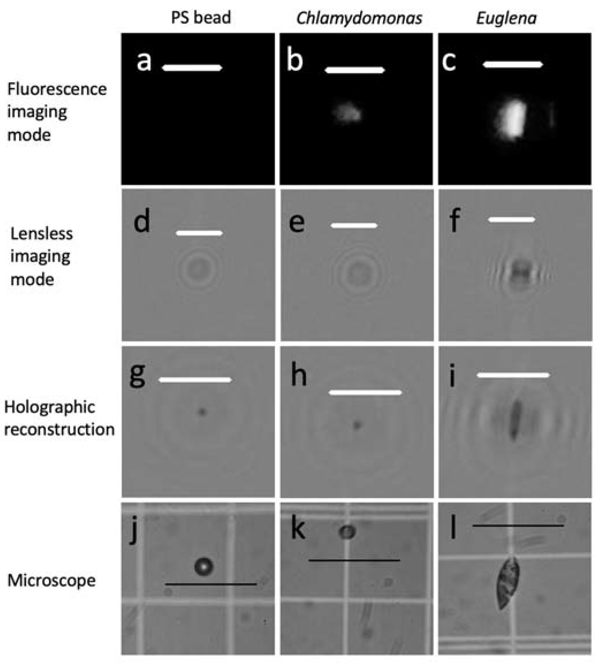
3.1. Particle Classification
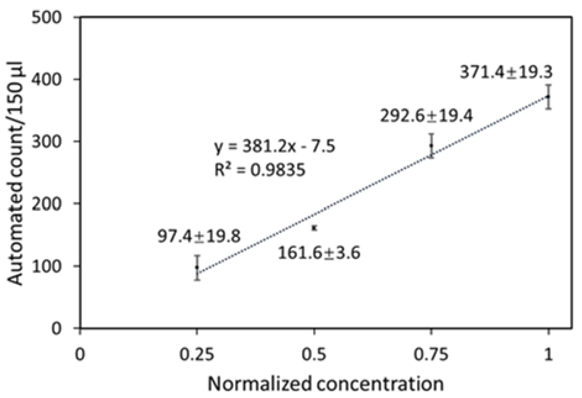
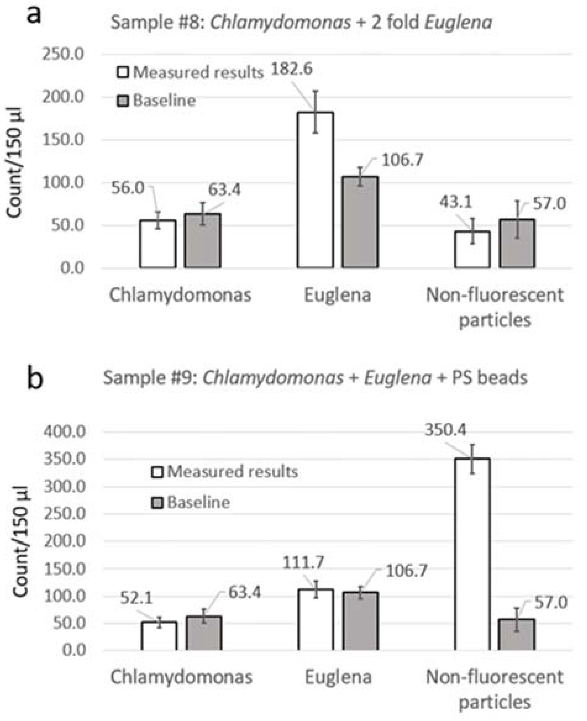
3.2. Particle Counting
4. Discussion
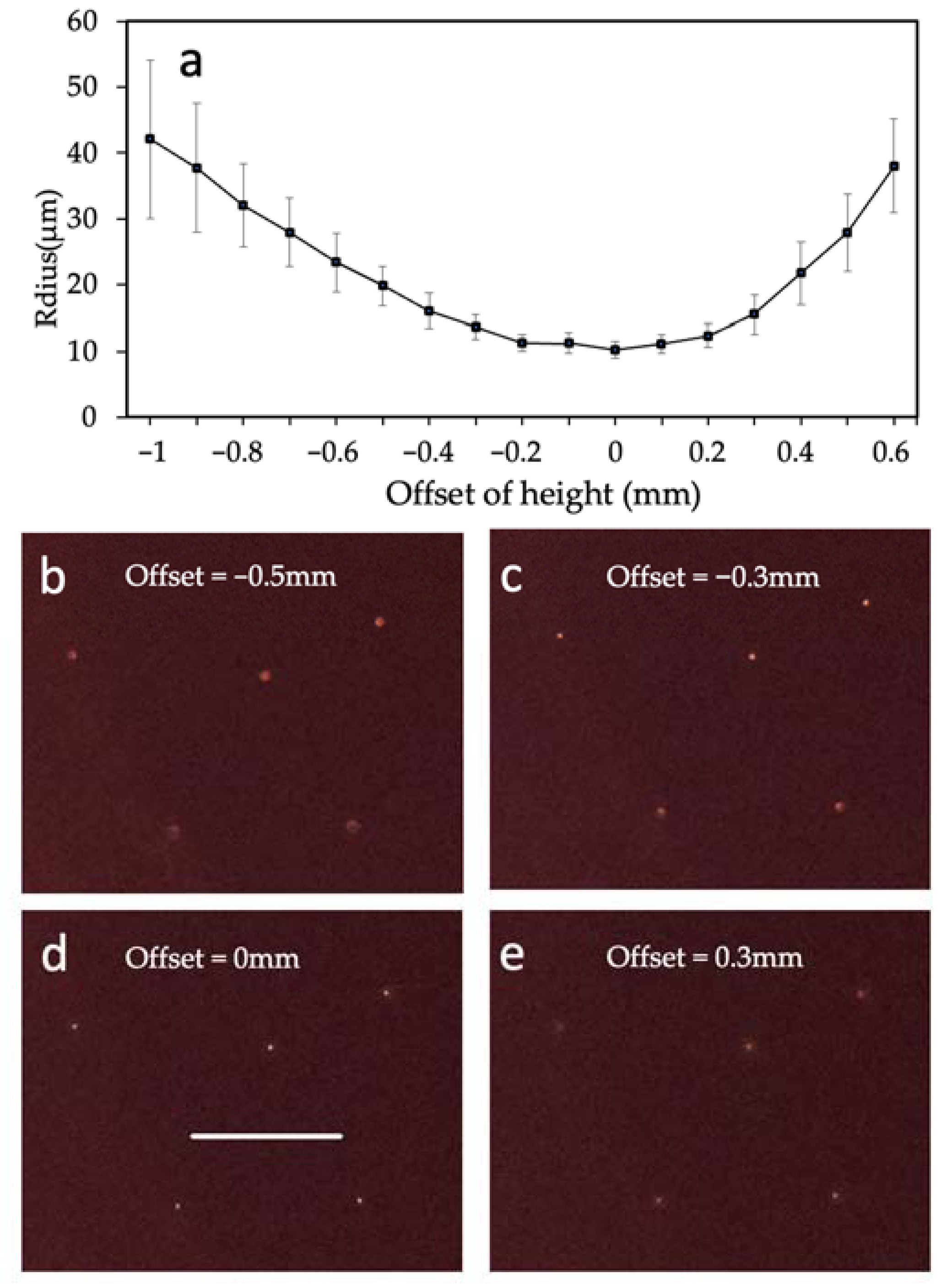
4.1. Performance of Fluorescence Mode
4.2. Volumetric Throughput
4.3. Analysis of Natural Water
5. Conclusions
Supplementary Materials
Author Contributions
Funding
Data Availability Statement
Acknowledgments
Conflicts of Interest
References
- Field, C.B.; Behrenfeld, M.J.; Randerson, J.T.; Falkowski, P. Primary production of the biosphere: Integrating terrestrial and oceanic components. Science 1998, 281, 237–240. [Google Scholar] [CrossRef] [Green Version]
- Carpenter, S.R.; Kitchell, J.F.; Hodgson, J.R.; Cochran, P.A.; Elser, J.J. Regulation of lake primary productivity by food web structure. Ecology 1987, 68, 1863–1876. [Google Scholar] [CrossRef] [Green Version]
- Benincà, E.; Huisman, J.; Heerkloss, R.; Jöhnk, K.; Branco, P. Chaos in a long-term experiment with a plankton community. Nature 2008, 451, 822–825. [Google Scholar] [CrossRef]
- Sahoo, D.; Seckbach, J. The Algae World; Springer: Dordrecht, The Netherlands, 2015. [Google Scholar]
- Grattan, L.M.; Holobaugh, S.; Morris, K.G., Jr. Harmful algal blooms and public health. Harmful Algae 2016, 57, 2–8. [Google Scholar] [CrossRef] [Green Version]
- Hallegraeff, G.M. A review of harmful algal blooms and their apparent global increase. Phycologia 1993, 32, 79–99. [Google Scholar] [CrossRef] [Green Version]
- Gallardo-Rodríguez, J.J.; Astuya-Villalón, A.; Llanos-Rivera, A.; Avello-Fontalba, V.; Ulloa-Jofré, V. A critical review on control methods for harmful algal blooms. Rev. Aquacult. 2019, 11, 661–684. [Google Scholar] [CrossRef]
- Martin, J.L.; Hanke, A.R.; LeGresley, M.M. Long term phytoplankton monitoring, including harmful algal blooms, in the Bay of Fundy, eastern Canada. J. Sea Res. 2009, 61, 76–83. [Google Scholar] [CrossRef]
- Lee, J.H.W.; Hodgkiss, I.J.; Wong, K.T.M.; Lam, I.H.Y. Real time observations of coastal algal blooms by an early warning system. Estuar. Coast. Shelf Sci. 2005, 65, 172–190. [Google Scholar] [CrossRef]
- Lomax, A.S.; Corso, W.; Etro, J.F. Employing unmanned aerial vehicles (UAVs) as an element of the Integrated Ocean Observing System. In Proceedings of the OCEANS 2005 MTS/IEEE, Washington, DC, USA, 17–23 September 2005; pp. 184–190. [Google Scholar]
- Coltelli, P.; Barsanti, L.; Evangelista, V.; Frassanito, A.M.; Gualtieri, P. Water monitoring: Automated and real time identification and classification of algae using digital microscopy. Environ. Sci. 2014, 16, 2656–2665. [Google Scholar] [CrossRef] [PubMed]
- Wilde, E.W.; Fliermans, C.B. Fluorescence microscopy for algal studies. Trans. Am. Microsc. Soc. 1979, 98, 96–102. [Google Scholar] [CrossRef]
- Beutler, M.; Wiltshire, K.H.; Meyer, B.; Moldaenke, C.; Lüring, C. A fluorometric method for the differentiation of algal populations in vivo and in situ. Photosynth. Res. 2002, 72, 39–53. [Google Scholar] [CrossRef]
- Izydorczyk, K.; Carpentier, C.; Mrówczyński, J.; Wagenvoort, A.; Jurczak, T.; Tarczyńska, M. Establishment of an Alert Level Framework for cyanobacteria in drinking water resources by using the Algae Online Analyser for monitoring cyanobacterial chlorophyll a. Water Res. 2009, 43, 989–996. [Google Scholar] [CrossRef]
- Shin, Y.H.; Barnett, J.Z.; Gutierrez-Wing, M.T.; Rusch, K.A.; Choi, J.W. A hand-held fluorescent sensor platform for selectively estimating green algae and cyanobacteria biomass. Sens. Actuators B Chem. 2018, 262, 938–946. [Google Scholar] [CrossRef]
- Wert, E.C.; Dong, M.M.; Rosario-Ortiz, F.L. Using digital flow cytometry to assess the degradation of three cyanobacteria species after oxidation processes. Water Res. 2013, 47, 3752–3761. [Google Scholar] [CrossRef] [PubMed]
- Wu, J.; Li, J.; Chan, R.K.Y. A light sheet based high throughput 3D-imaging flow cytometer for phytoplankton analysis. Opt. Express 2013, 21, 14474–14480. [Google Scholar] [CrossRef]
- Park, J.; Kim, Y.; Kim, M.; Lee, W.H. A novel method for cell counting of Microcystis colonies in water resources using a digital imaging flow cytometer and microscope. Environ. Eng. Res. 2019, 24, 397–403. [Google Scholar] [CrossRef]
- Rutten, T.P.A.; Sandee, B.; Hofman, A.R.T. Phytoplankton monitoring by high performance flow cytometry: A successful approach? Cytom. Part A J. Int. Soc. Anal. Cytol. 2005, 64, 16–26. [Google Scholar] [CrossRef]
- Han, Y.; Gu, Y.; Zhang, A.C.; Lo, Y.H. Imaging technologies for flow cytometry. Lab Chip 2016, 16, 4639–4647. [Google Scholar] [CrossRef] [PubMed]
- Dashkova, V.; Malashenkov, D.; Poulton, N.; Vorobjev, I.; Barteneva, N.S. Imaging flow cytometry for phytoplankton analysis. Methods 2017, 112, 188–200. [Google Scholar] [CrossRef]
- Olson, R.J.; Sosik, H.M. A submersible imaging-in-flow instrument to analyze nano-and microplankton: Imaging FlowCytobot. Limnol. Oceanogr. Methods 2007, 5, 195–203. [Google Scholar] [CrossRef] [Green Version]
- Ozcan, A.; McLeod, E. Lensless imaging and sensing. Annu. Rev. Biomed. Eng. 2016, 18, 77–102. [Google Scholar] [CrossRef] [Green Version]
- Roy, M.; Seo, D.; Oh, S.; Yang, J.W.; Seo, S. A review of recent progress in lens-free imaging and sensing. Biosens. Bioelectron. 2017, 88, 130–143. [Google Scholar] [CrossRef] [PubMed]
- Seo, S.; Su, T.W.; Tseng, D.K.; Erlinger, A.; Ozcan, A. Lensfree holographic imaging for on-chip cytometry and diagnostics. Lab Chip 2009, 9, 777–787. [Google Scholar] [CrossRef] [PubMed]
- Mudanyali, O.; Bishara, W.; Ozcan, A. Lensfree super-resolution holographic microscopy using wetting films on a chip. Opt. Express 2011, 19, 17378–17389. [Google Scholar] [CrossRef] [PubMed]
- Merola, F.; Memmolo, P.; Bianco, V.; Paturzo, M.; Mazzocchi, M.G.; Ferraro, P. Searching and identifying microplastics in marine environment by digital holography. Eur. Phys. J. Plus 2018, 133, 1–6. [Google Scholar] [CrossRef]
- Kun, J.; Smieja, M.; Xiong, B.; Soleymani, L.; Fang, Q. The Use of Motion Analysis as Particle Biomarkers in Lensless Optofluidic Projection Imaging for Point of Care Urine Analysis. Sci. Rep. 2019, 9, 17255. [Google Scholar] [CrossRef] [Green Version]
- Mahoney, E.; Kun, J.; Smieja, M.; Fang, Q. Point-of-care urinalysis with emerging sensing and imaging technologies. J. Electrochem. Soc. 2019, 167, 037518. [Google Scholar] [CrossRef]
- Lu, C.H.; Shih, T.S.; Shih, P.C.; Pendharkar, G.P.; Liu, C.E. Finger-powered agglutination lab chip with CMOS image sensing for rapid point-of-care diagnosis applications. Lab Chip 2020, 20, 424–433. [Google Scholar] [CrossRef]
- Göröcs, Z.; Tamamitsu, M.; Bianco, V.; Wolf, P.; Roy, S.; Shindo, K.; Yanny, K.; Wu, Y.; Koydemir, H.C.; Rivenson, Y.; et al. A deep learning-enabled portable imaging flow cytometer for cost-effective, high-throughput, and label-free analysis of natural water samples. Light Sci. Appl. 2018, 7, 66. [Google Scholar] [CrossRef]
- Boddy, L.; Morris, C.W.; Wilkins, M.F.; Al-Haddad, L.; Tarran, G.A.; Jonker, R.R.; Burkill, P.H. Identification of 72 phytoplankton species by radial basis function neural network analysis of flow cytometric data. Mar. Ecol. Prog. Ser. 2000, 195, 47–59. [Google Scholar] [CrossRef]
- Coskun, A.F.; Su, T.W.; Ozcan, A. Wide field-of-view lens-free fluorescent imaging on a chip. Lab Chip 2010, 10, 824–827. [Google Scholar] [CrossRef] [PubMed] [Green Version]
- Shanmugam, A.; Salthouse, C. Lensless fluorescence imaging with height calculation. J. Biomed. Opt. 2014, 19, 016002. [Google Scholar] [CrossRef] [PubMed] [Green Version]
- Paiè, P.; Vázquez, R.M.; Osellame, R.; Bragheri, F.; Bassi, A. Microfluidic Based Optical Microscopes on Chip. Cytom. Part A 2018, 93, 987–996. [Google Scholar] [CrossRef] [PubMed]
- Pang, S.; Han, C.; Lee, L.M.; Yang, C. Fluorescence microscopy imaging with a Fresnel zone plate array based optofluidic microscope. Lab Chip 2011, 11, 3698–3702. [Google Scholar] [CrossRef] [Green Version]
- Sommer, U.; Charalampous, E.; Genitsaris, S.; Moustaka-Gouni, M. Benefits, costs and taxonomic distribution of marine phytoplankton body size. J. Plankton Res. 2017, 39, 494–508. [Google Scholar] [CrossRef]
- Borowitzka, M. Microalgae in Health and Disease Prevention; Academic Press: Cambridge, MA, USA, 2018. [Google Scholar]
- Salomé, P.A.; Merchant, S.S. A Series of Fortunate Events: Introducing Chlamydomonas as a Reference Organism. Plant Cell 2019, 31, 1682–1707. [Google Scholar] [CrossRef] [Green Version]
- Toyama, T.; Kasuya, M.; Hanaoka, T.; Kobayashi, N.; Tanaka, Y. Growth promotion of three microalgae, Chlamydomonas reinhardtii, Chlorella vulgaris and Euglena gracilis, by in situ indigenous bacteria in wastewater effluent. Biotechnol. Biofuels 2018, 11, 176. [Google Scholar] [CrossRef] [Green Version]
- McCree, K.J. The action spectrum, absorptance and quantum yield of photosynthesis in crop plants. Agric. Meteorol. 1972, 9, 191–216. [Google Scholar] [CrossRef]
- Dadi, H.S.; Pillutla, G.K.M. Improved face recognition rate using HOG features and SVM classifier. IOSR J. Electron. Commun. Eng. 2016, 11, 34–44. [Google Scholar] [CrossRef]
- Kristan, M.; Leonardis, A.; Matas, J.; Felsberg, M.; Pflugfelder, M.; Cehovin Zajc, L.; Vojir, T.; Bhat, G.; Lukezic, A.; Eldesokey, A.; et al. The sixth visual object tracking vot2018 challenge results. In Proceedings of the European Conference on Computer Vision, Munich, Germany, 8–14 September 2018. [Google Scholar]
- Latychevskaia, T.; Fink, H. Practical algorithms for simulation and reconstruction of digital in-line holograms. Appl. Opt. 2015, 54, 2424–2434. [Google Scholar] [CrossRef] [Green Version]
- Ector, L. River Algae; Springer International Publishing: Cham, Switzerland, 2016. [Google Scholar]
- Xiong, B.; Fang, Q. Luminescence lifetime imaging using a cellphone camera with an electronic rolling shutter. Opt. Lett. 2020, 45, 81–84. [Google Scholar] [CrossRef]
- Geelen, B.; Tack, N.; Lambrechts, A. A compact snapshot multispectral imager with a monolithically integrated per-pixel filter mosaic. In Proceedings of the Advanced Fabrication Technologies for Micro/Nano Optics and Photonics VII, San Francisco, CA, USA, 7 March 2014; Volume 8974. [Google Scholar]
- Zhang, Y.; Xu, C.-Q.; Guo, T.; Hong, L. An automated bacterial concentration and recovery system for pre-enrichment required in rapid Escherichia coli detection. Sci. Rep. 2018, 8, 17808. [Google Scholar] [CrossRef] [PubMed]


| Sample ID | Chlamydomonas | Euglena | PS Beads | BBM | Total |
|---|---|---|---|---|---|
| # 1 | 0 mL 0 mL | 0 mL | 1 mL | 29 mL | 30 mL |
| # 2 | 2 mL | 0 mL | 28 mL | 30 mL | |
| # 3 | 1.5 mL | 0 mL | 0 mL | 28.5 mL | 30 mL |
| # 4 | 0.5 mL | 0 mL | 0 mL | 29.5 mL | 30 mL |
| # 5 | 1 mL | 0 mL | 0 mL | 29 mL | 30 mL |
| # 6 | 2 mL | 0 mL | 0 mL | 28 mL | 30 mL |
| # 7 | 0.33 mL | 0.67 mL | 0 mL | 29 mL | 30 mL |
| # 8 | 0.33 mL | 1.33 mL | 0 mL | 28.33 mL | 30 mL |
| # 9 | 0.33 mL | 0.67 mL | 0.4 mL | 28.67 mL | 30 mL |
| Class | Predicted: Chlamydomonas | Predicted: Euglena | Predicted: PS Bead |
|---|---|---|---|
| Actual: Chlamydomonas | 0.936 | 0.005 | 0.059 |
| Actual: Euglena | 0.016 | 0.944 | 0.041 |
| Actual: PS bead | 0.000 | 0.000 | 1.000 |
| Class | Predicted: Chlamydomonas | Predicted: Euglena | Predicted: PS Bead |
|---|---|---|---|
| Actual: Chlamydomonas | 0.831 | 0.005 | 0.163 |
| Actual: Euglena | 0.016 | 0.897 | 0.087 |
| Actual: PS bead | \ | \ | \ |
| Class | Predicted: Chlamydomonas | Predicted: Euglena | Predicted: PS Bead |
|---|---|---|---|
| Actual: Chlamydomonas | 0.817 | 0.028 | 0.155 |
| Actual: Euglena | 0.043 | 0.924 | 0.033 |
| Actual: PS bead | 0.040 | 0.022 | 0.937 |
Publisher’s Note: MDPI stays neutral with regard to jurisdictional claims in published maps and institutional affiliations. |
© 2021 by the authors. Licensee MDPI, Basel, Switzerland. This article is an open access article distributed under the terms and conditions of the Creative Commons Attribution (CC BY) license (https://creativecommons.org/licenses/by/4.0/).
Share and Cite
Xiong, B.; Hong, T.; Schellhorn, H.; Fang, Q. Dual-Modality Imaging Microfluidic Cytometer for Onsite Detection of Phytoplankton. Photonics 2021, 8, 435. https://doi.org/10.3390/photonics8100435
Xiong B, Hong T, Schellhorn H, Fang Q. Dual-Modality Imaging Microfluidic Cytometer for Onsite Detection of Phytoplankton. Photonics. 2021; 8(10):435. https://doi.org/10.3390/photonics8100435
Chicago/Turabian StyleXiong, Bo, Tianqi Hong, Herbert Schellhorn, and Qiyin Fang. 2021. "Dual-Modality Imaging Microfluidic Cytometer for Onsite Detection of Phytoplankton" Photonics 8, no. 10: 435. https://doi.org/10.3390/photonics8100435
APA StyleXiong, B., Hong, T., Schellhorn, H., & Fang, Q. (2021). Dual-Modality Imaging Microfluidic Cytometer for Onsite Detection of Phytoplankton. Photonics, 8(10), 435. https://doi.org/10.3390/photonics8100435