Target Detection Method for Low-Resolution Remote Sensing Image Based on ESRGAN and ReDet

Abstract

With the widespread use of remote sensing images, low-resolution target detection in remote sensing images has become a hot research topic in the field of computer vision. In this paper, we propose a Target Detection on Super-Resolution Reconstruction (TDoSR) method to solve the problem of low target recognition rates in low-resolution remote sensing images under foggy conditions. The TDoSR method uses the Enhanced Super-Resolution Generative Adversarial Network (ESRGAN) to perform defogging and super-resolution reconstruction of foggy low-resolution remote sensing images. In the target detection part, the Rotation Equivariant Detector (ReDet) algorithm, which has a higher recognition rate at this stage, is used to identify and classify various types of targets. While a large number of experiments have been carried out on the remote sensing image dataset DOTA-v1.5, the results of this paper suggest that the proposed method achieves good results in the target detection of low-resolution foggy remote sensing images. The principal result of this paper demonstrates that the recognition rate of the TDoSR method increases by roughly 20% when compared with low-resolution foggy remote sensing images.

1. Introduction

The task of target detection in remote sensing images is to locate, recognize, or classify ground objects. With the advent of the Convolutional Neural Network (CNN) [1], computer vision has become a hot spot in the field of artificial intelligence, especially in image processing, which has recently experienced unprecedented development [2,3]. Whether it is due to the low performance of some imaging equipment or the extreme weather conditions, the collected remote sensing images cannot satisfy the practice requirements with such low quality. The task of single image super-resolution (SISR) [4] processing is to recover a high-resolution image from a low-resolution image. Before the deep learning method was proposed, the Bicubic [4] method was usually used to deal with the problem of single image super-resolution. However, this method only used the pixel information of the low-resolution image itself, and all the pixels at each position were interpolated based on the information around the corresponding pixels so that the super-resolution image obtained by this method was unsatisfactory and had poor image quality. Learning a Deep Convolutional Network for Image Super-Resolution (SRCNN) [4] introduced CNN to the task of image super-resolution reconstruction for the first time. The network structure of the SRCNN only used three convolutional layers. Compared with the traditional reconstruction methods, the reconstruction effect of the image had improved but the details in the high-frequency parts of the image were still processed normally [5,6]. In response, Photo-Realistic Single Image Super-Resolution Using a Generative Adversarial Network (SRGAN) [7] applied the Generative Adversarial Network (GAN) [8] to solve the problem of super-resolution. The SRGAN added perceptual loss and adversarial loss to the GAN framework to increase the authenticity of the generated images. While the visual effect of the super-resolution image reconstructed by the SRGAN had been improved, there was still a significant gap when compared to the real image [7,9,10,11]. The Enhanced Deep Residual Networks for Single Image Super-Resolution (EDSR) [12] removed the batch normalization layer (BN) [10] in the network on the basis of SRGAN, expanded the model size, and obtained better super-division images after training. While the performance of the above-mentioned methods in dealing with the super-resolution reconstruction of remote sensing images was not very good, the Enhanced Super-Resolution Generative Adversarial Networks (ESRGAN) [13] achieved a perfect effect. The ESRGAN [13] made three improvements on the basis of the SRGAN. First, the Residual in Residual Dense Block (RRDB), which had a larger capacity and was easier to train, was introduced into the network and replaced the original basic residuals. Second, the BN layer was removed [10] and the GAN network was improved to a Relativistic average GAN (RaGAN) [13] network. ESRGAN’s discriminator could then predict whether an image was more real after learning rather than judging whether an image was true or false. Third, the perceptual domain loss function was modified and the VGG feature [14] before its activation was used. After these improvements, the image reconstructed by the ESRGAN had more realistic texture details and attained a better visual effect. Previously, the ESRGAN was not applied to low-resolution foggy remote sensing images. The experiments in this paper prove that the ESRGAN is very suitable for the super-resolution reconstruction of remote sensing images. Kwan et al. have proposed a method to enhance low-resolution images based on a point spread function, which has provided a new direction for future research [15].

Through the ESRGAN network, high-quality super-resolution images are obtained and target detection is performed on the super-resolution images. In this paper, the target detection network selected the Rotating Equivariant Detector (ReDet) [16] and the results were displayed in Oriented Bounding Boxes (OBBs) [17,18]. Rotating the feature map obtained by inputting an image into the CNN was different from the feature map obtained by inputting the image into the CNN after the rotation. The ReDet detection method consists of two parts, the rotation equivariant feature extraction and the rotation invariant feature extraction [17,19]. Finally, the combination of these two methods realizes the detection of small and dim targets in the remote sensing images with higher accuracy.

2. Related Work

Currently there are no open source and complete low-resolution remote sensing image datasets. Therefore, the public remote sensing image data set named DOTA-v1.5 [20] has been selected for this research. The Bicubic method is used to down-sample the DOTA data set so to obtain low-resolution remote sensing images. Then, the down-sampled remote sensing images are artificially simulated and fogged by the mainstream RGB channel synthesis fog method. This obtained low-quality image data set is then used for the following super-resolution reconstruction research.

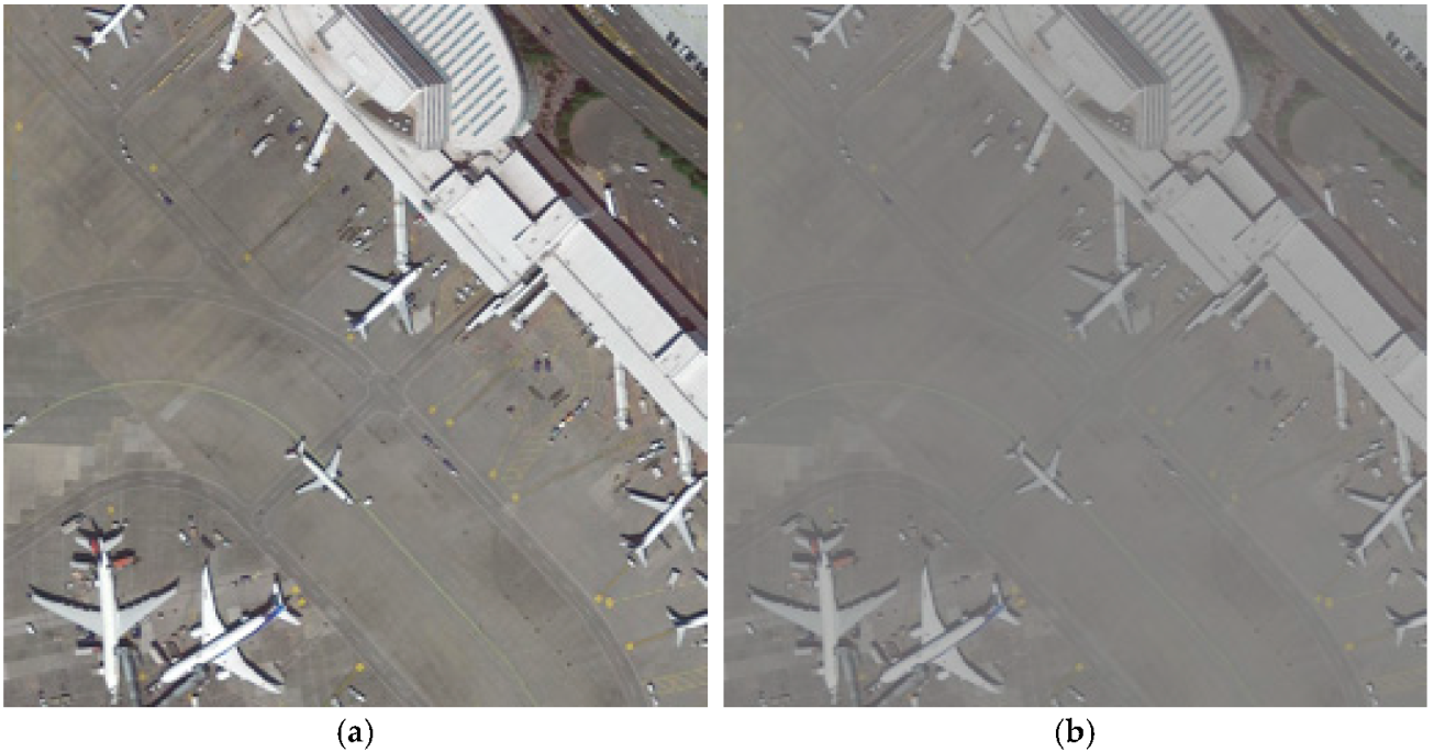
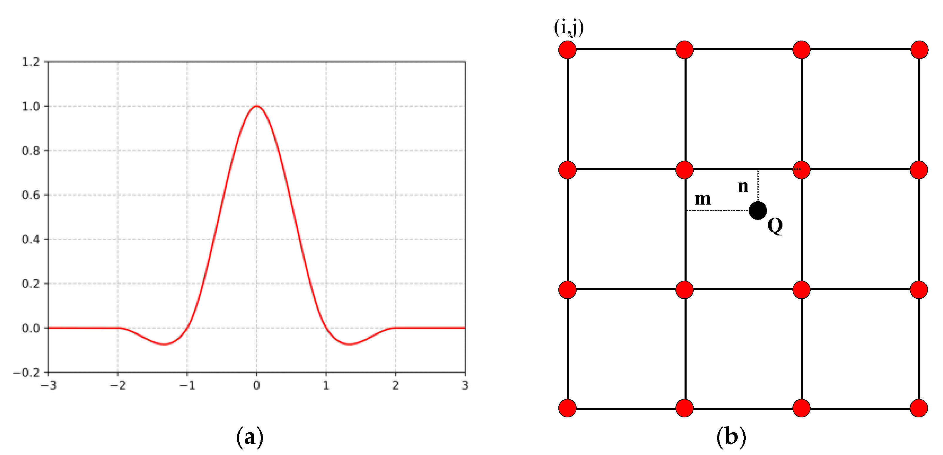
2.1. Bicubic Interpolation

Bicubic interpolation, also called cubic convolution interpolation, is a complicated interpolation algorithm. This algorithm uses the gray values of 16 points around those points that will be sampled for cubic interpolation. Not only are the gray effects of four directly adjacent points considered, but also the influence of the gray value change rates between the adjacent points [21]. This paper uses this algorithm to down-sample the remote sensing images.

Suppose that the size of the source image $A$ to be processed is $u\times v$, and the size of the target image $B$ scaled from $A$ is $U\times V$. According to the zoom ratio, the corresponding coordinate of a point $\left(X,Y\right)$ on the target image $B$ on the source image $A$ is $\left(x,y\right)=A[X\times \left(\frac{u}{U}\right),Y\times \left(\frac{v}{V}\right)]$. In the bicubic interpolation, the 16 pixels closest to $\left(x,y\right)$ are selected when calculating the parameters of the pixel value at $\left(X,Y\right)$ on the target image $B$. The algorithm needs to select an interpolation basis function to fit the data, and the commonly used interpolation basis function expression is shown in Formula 1. The image of the interpolation basis function is shown in Figure 1a, while Figure 1b is the schematic diagram of the bicubic algorithm.

$$W(x)=\{\begin{array}{cc}1.5|x{|}^3-2.5|x{|}^2+1\hfill & \mathrm{for}\left|x\right|\le 1\hfill \\ -0.5|x{|}^3+2.5|x{|}^2-4\left|x\right|+2\hfill & \mathrm{for}1<\left|x\right|<2\hfill \\ 0\hfill & \left|x\right|\ge 2\end{array}$$

(1)

The $Q$ point is the source image coordinate point corresponding to the point $(X\text{,}Y)$ on the target image $B$ after being reduced several times; then, the coefficients of the 16 points around point $Q$ are calculated, and the pixel value of point $Q$ is obtained after weighting, as shown in Figure 1b. As is shown, where m is the distance between the point and the abscissa of the upper left corner point, and n is the distance between the point and the ordinate of the upper left corner point. To find the coefficient corresponding to each coordinate point:

The distances between the four points in the $X$ axis direction of each row and the $Q$ point are $1+m,m,1-m,2-m.$

The distances between the four points in the $Y$ axis direction of each row and the $Q$ point are $1+n,n,1-n,2-n.$

From the interpolation basis function operation, if the row coefficient corresponding to point $\left(i,j\right)$ is $W\left(1+m\right)$ and the corresponding column coefficient is $W\left(1+n\right)$, then the coefficient of this point is $K_{0,0}=W(1+m)·W(1+n)$.

The coefficients of the remaining points are calculated as above, and so the coefficients of the four points in the first row are:

$$\begin{array}{c}{K}_0{}_{,0}=W(1+m)·W(1+n),K_{1,0}=W(m)·W(1+n),\\ K_{2,0}=W(1-m)·W(1+n),K_{1,0}=W(2-m)·W(1+n).\end{array}$$

(2)

The coefficients of the four points in the second row are:

$$\begin{array}{c}{K}_{0,1}=W(1+m)·W(n),K_{1,1}=W(m)·W(n),\\ K_{2,1}=W(1-m)·W(n),K_{3,1}=W(2-m)·W(n).\end{array}$$

(3)

The coefficients of the four points in the third row are:

$$\begin{array}{c}{K}_{0,2}=W(1+m)·W(1-n),K_{1,2}=W(m)·W(1-n),\\ K_{2,2}=W(1-m)·W(1-n),K_{3,2}=W(2-m)·W(1-n).\end{array}$$

(4)

The coefficients of the four points in the fourth row are:

$$\begin{array}{c}{K}_{0,3}=W(1+m)·W(2-n),K_{1,3}=W(m)·W(2-n),\\ K_{2,3}=W(1-m)·W(2-n),K_{3,3}=W(2-m)·W(2-n).\end{array}$$

(5)

Therefore, the pixel value of the $Q$ point can be obtained by adding the pixel values of the 16 points multiplied by the corresponding coefficients. Then, the down-sampled image can be obtained by the Bicubic interpolation algorithm.

Finally, the down-sampled images are artificially fogged to obtain low-resolution remote sensing images under foggy conditions, as shown in Figure 2.

2.2. Effective Algorithms for SISR

The following will introduce some of the effective algorithms used in recent years for single image super-resolution reconstruction.

2.2.1. Generative Adversarial Network (GAN)

The generative confrontation network [8] is mainly composed of two network models: the generator network $G$ and the discriminator network $D$. The main function of the generator network is to receive a random noise $z$ and generate an image similar to the original through this noise. The role of the discriminator network is mainly to determine whether an image is real or synthesized by a generator. The two network models compete to improve their algorithmic capabilities until the discriminator cannot determine whether the composite image is true or false.

The cost function of generating a confrontation network is: $V\left(D,G\right)$

$$\underset{G}{\min }\underset{D}{\max }V(D,G)={\mathbb{E}}_{x~p_{\mathrm{data}}(x)}[\log D(x)]+{\mathbb{E}}_{z~p_z(z)}[\log (1-D(G(z)))]$$

(6)

where $x$ represents a real image, $z$ represents the random noise input to the generator $G$, and $G(z)$ represents the image generated by the generator $G$. $D(x)$ represents the probability of the discriminator $D$ to determine whether the real image is indeed real. For $D$, the closer $D(x)$ is to 1, the better. $D(G(z))$ represents the probability that $D$ judges whether the image generated by $G$ is real. $G$ hopes that $D(G(z))$ is as large as possible, and at the time $V\left(D,G\right)$ will become smaller. Finally, $D$ hopes that the larger is the $D(x)$, the smaller the $D(G(z))$, at time $V\left(D,G\right)$ it will become larger.

2.2.2. SRGAN

SRGAN [7] applied the GAN [8] to the task of processing the image super-resolution reconstruction for the first time and made improvements in the loss function. SRGAN’s network model is divided into three parts: generator, discriminator, and VGG [14] network. In the training process, the generator and the discriminator alternate against training and iterating continuously. The VGG [14,22,23] network only participates in the calculation of $Loss$.

The generator of the SRGAN is an improvement made on the basis of SRResNet. The generator network part contains multiple residual blocks, and each residual block contains two A convolutional layers which are connected to batch normalization (BN) [10] after the convolutional layer. Take the PReLU as the activation function and choose two $2\times$ sub-pixel convolution layers to increase the feature size [6]. The discriminator network part of the SRGAN contains 8 convolutional layers. As the number of network layers deepens, the number of features continues to increase while the feature size continues to decrease. LeakyReLU is selected as the activation function [22] and finally passes through two fully connected layers and the final sigmoid. The activation function is used to predict the probability of whether the generated image is a real image.

The loss function of the SRGAN is divided into generator loss and discriminator loss. The generator loss consists of content loss and counter loss. The loss function of the generator is as follows:

$$l^{SR}=l_X^{SR}+{10}^{-3}{l}_{Gen}^{SR}$$

(7)

where $l_X^{SR}$ is a content loss and $l_{Gen}^{SR}$ is a confrontation loss. The content loss includes the MSE loss [6,21] and the VGG loss. The MSE loss is used to calculate the matching degree between pixels, and the VGG loss is used to calculate the matching degree of a feature layer. Using MSE can get a good performance evaluation index, but the super-resolution reconstructed image obtained only using the MSE loss loses more high-frequency information. The purpose of adding the VGG loss is to more effectively recover the high-frequency information of the image.

The calculation of the MSE loss is as follows:

$$l_{MSE}^{SR}=\frac{1}{r^{2}WH}{\displaystyle \sum _{x=1}^{rW}{\displaystyle \sum _{y=1}^{rH}{\left(I_{x,y}^{HR}-G_{{\theta }_G}{\left(I^{LR}\right)}_{x,y}\right)}^2}}$$

(8)

where $W$ represents the width of the image, $H$ represents the height of the image, $I^{HR}$ is the real high-resolution image, and $I^{LR}$ is the low-resolution image corresponding to the real high-resolution image.

The calculation of the VGG loss is as follows:

$$l_{VGG/i.j}^{SR}=\frac{1}{W_{i,j}{H}_{i,j}}{\displaystyle \sum _{x=1}^{W_{i,j}}{\displaystyle \sum _{y=1}^{H_{i,j}}({\varphi }_{i,j}{\left(I^{HR}\right)}_{x,y}}}{-{\varphi }_{i,j}{\left(G_{{\theta }_G}\left(I^{LR}\right)\right)}_{x,y})}^2$$

(9)

where ${\varphi }_{i,j}$ represents the feature map obtained before the $i$ maximum pooling layer of the $j$ convolution of the VGG network, and $W_{i,j}$ and $H_{i,j}$ are the dimensions of the corresponding feature map in the VGG network.

The counter loss of the generator is calculated as follows:

$$l_{Gen}^{SR}={\displaystyle \sum _{n=1}^N-}\log D_{{\theta }_D}\left(G_{{\theta }_G}\left(I^{LR}\right)\right)$$

(10)

where $D_{{\theta }_D}\left(G_{{\theta }_G}\left(I^{LR}\right)\right)$ is the estimated probability that the reconstructed image and $G_{{\theta }_G}\left(I^{LR}\right)$ is a natural HR image [8].

The optimization of generator network $G_{{\theta }_G}$ and discriminator network $D_{{\theta }_D}$ is as follows:

$${\min }_{{\theta }_G}{\max }_{{\theta }_D}{\mathbb{E}}_{I^{HR}~p_{\mathrm{train}}\left(I^{HR}\right)}\left[\log D_{{\theta }_D}\left(I^{HR}\right)\right]+{\mathbb{E}}_{I^{LR}~p_G\left(I^{LR}\right)}[\log \left(1-D_{{\theta }_D}\left(G_{{\theta }_G}\left(I^{LR}\right)\right)\right]$$

(11)

where $I^{HR}$ is the real high-resolution image, $I^{LR}$ is the low-resolution image corresponding to the real high-resolution image, and $I^{SR}$ is the super-resolution after inputting the low-resolution image into the SRGAN network and the super-resolution reconstruction image.

However, the super-resolution image reconstructed by the SRGAN still has a large gap with the real image and it cannot recover more real textural details or more semantic information.

2.2.3. EDSR

Compared with the SRGAN, the EDSR removes the BN layer on the basis of its network. For the task of the image super-resolution reconstruction, the image generated by the network is required to be consistent with the input source image in terms of brightness, contrast, and color, while only the resolution and some of the details are changed. In the processing of images, the BN layer is equivalent to contrast stretching. The color distribution of the image is normalized, which destroys the original contrast information of the image [12]. Therefore, the performance of the BN layer in the image super-resolution is not good. The addition of the BN layer increases the training time, thereby making the training unstable or even divergent.

The model performance of the EDSR is improved by removing the BN layer in the residual network, by increasing the number of residual layers from 16 to 32, and then expanding the model size. The EDSR uses the loss function of $L1$ [23] norm style to optimize the network model. During training, we first train the low-multiple up-sampling model, and then use the obtained parameters to initialize the high-multiple up-sampling model, which not only reduces the training time of the high-multiple up-sampling model but also achieves a very high level training effect.

The EDSR has achieved a good effect in the super-resolution reconstruction task, but there is still a large gap in edge detail from the real image.

3. Experimental Method

Through the research and comparison of image super-resolution reconstruction algorithms, the ESRGAN algorithm is selected for the following research and has the best effect in the field of remote sensing image reconstruction thus far. Through the super-resolution processing of low-resolution remote sensing images, the generated super-resolution images are identified and classified. The flow chart of the whole set of identification is shown in Figure 3.

3.1. ESRGAN

ESRGAN’s [13] generator network refers to the SRResNet structure. The ESRGAN has two improvements on the basis of this generator network. First, it removes all the BN layers in the network. After removing the BN layers, the generalization ability of the model and the training speed are both improved. Second, the original residual block is changed to the Residual in Residual Dense Block (RRDB). The changed RRDB combines multi-layer residual networks and dense connections [12,24]. The previous algorithms for super-resolution reconstruction based on the GAN are used in the discriminator network to determine whether the image generated by the generator is true and natural [9]. The most important improvement of the ESRGAN discriminator network is the probability that it discriminates real images more realistically than fake images. The ESRGAN uses the VGG features before activation in the perceptual domain loss and overcomes two shortcomings. First, the features after activation are very sparse, especially in deep networks. This sparse activation provides a weaker supervision effect, which makes the generator network performance low. Second, the use of activated features causes the super-resolution reconstructed image to differ in brightness from the real image.

The ESRGAN uses a relative average discriminator, and the loss function of the discriminator is defined as:

$$L_D=-E_{x_r}\left[\log \left(D_{Ra}\left(x_r,x_f\right)\right)\right]-E_{x_f}\left[1-\log \left(D_{Ra}\left(x_f,x_r\right)\right)\right]$$

(12)

where x_r is the real image, $x_f$ is the original low-resolution image generated by the generator, $D_{Ra}\left(x_r,x_f\right)$ is the difference between the real image and the average value of the generated image, and $D_{Ra}\left(x_f,x_r\right)$ is the difference between the average value of the generated image and the real image.

The counter loss function of the generator is defined as:

$$L_G=L_{\mathrm{percep}}+\lambda L_G^{Ra}+\eta L_1$$

(13)

where $L_{\mathrm{percep}}$ is the perceptual domain loss, $L_G^{Ra}$ is the counter loss of the generator, and $L_1$ is the pixel-wise loss, $\left(x,y,w,h,\theta \right)$ and $\lambda =5\times {10}^{-3},\eta =0.01$ in the experiment.

3.2. Rotating Equivariant Detector

Unlike natural images, targets in aerial images are usually arbitrarily oriented. In order to overcome this difficulty, researchers generally represent the detection of aerial targets as a task of orientation detection that relies on the characterization of oriented bounding boxes (OBBs) [17] instead of horizontal bounding boxes (HBBs) [17].

ReDet uses rotating equivariant networks instead of traditional convolutional neural networks to extract the features. Compared with convolutional neural networks, which share translation weights, rotating equivariant networks share translation and rotation weights. ReDet uses a rotating equivariant network and ResNet with Feature Pyramid Networks (FPN) [25] as the backbone to realize a rotating equivariant backbone network, named Rotation-equivariant ResNet (ReResNet) so to extract the features of the rotation equivariant, which can accurately predict the orientation and significantly reduce the model size.

Take the horizontal RoIs (HRoI) output by the backbone network through the Region Proposal Network (RPN) [26] as the input, shrink it to 10 channels after one convolution, enter the fully connected layer, and output a 5-dimensional vector. The gt value of each dimension is as follows:

$$\begin{array}{c}{t}_x^{\ast }=\frac{1}{w_r}\left(\left(x^{\ast }-x_r\right)\cos {\theta }_r+\left(y^{\ast }-y_r\right)\sin {\theta }_r\right);\\ t_y^{\ast }=\frac{1}{h_r}\left(\left(y^{\ast }-y_r\right)\cos {\theta }_r-\left(x^{\ast }-x_r\right)\sin {\theta }_r\right);\\ t_w^{\ast }=\log \frac{w^{\ast }}{w_r};t_h^{\ast }=\log \frac{h^{\ast }}{h_r};\\ t_{\theta }^{\ast }=\frac{1}{2\pi }\left(\left({\theta }^{\ast }-{\theta }_r\right)\mathrm{mod}2\pi \right)\end{array}$$

(14)

where the five values are the gt value of RRoI and the offset of HRoI. Use these offsets as inputs to enter the decoder module and to decode the relevant parameters of RRoI, namely $\left(x,y,w,h,\theta \right)$. This can make the final RRoI as close as possible to the gt value, which reduces the number of parameters and improves the performance of the rotating frame detection.

Concurrently, ReDet designed a novel Rotation-invariant RoI Align (RiRoI Align). RiRoI Align includes both spatial alignment and direction alignment. Its task is to transform the rotation equivariant features so to obtain rotation-invariant features (instance level), the so-called rotation Unchanging means that, no matter how the input changes (rotation), the output is always the same. RiRoI Align generates RoI rotation invariant features from the feature map that are equal to the rotation.

Given an input image in ReDet, we input it into the ReResNet network, extract the rotational equivariant features, use RPN to generate HRoIs, and then use RoI Transformer to convert HRoIs to RRoIs $\left(x,y,w,h,\theta \right)$. Finally, RiRoI Align is used to extract rotation invariant features for RoI classification and bounding box regression.

3.3. TDoSR

In this method, the down-sampling and super-resolution reconstruction of the image are carried out according to the scale factor ${\times }^{}4$. As the size of the image in the DOTA dataset is too large, it was cropped to a ${1024}^{}{\times }^{}1024$ size image before the experiment. Then we use the MATLAB Bicubic algorithm to down-sample the original high-definition remote sensing image to obtain a low-resolution remote sensing image with a size of ${256}^{}{\times }^{}256$. The method of the RGB channel synthesizing fog in MATLAB is used to artificially simulate and add fog to low-resolution remote sensing images.

The training process is divided into two stages. First, we train a PSNR-oriented model with the L1 loss. The learning rate is initialized as $2^{}{\times }^{}{10}^{-4}$ and decayed by a factor of 2 every $2^{}{\times }^{}{10}^5$ iterations. We then employ the trained PSNR-oriented model as an initialization for the generator. The generator is trained using the loss function in Equation (9) with $\lambda =5^{}{\times }^{}{10}^{-3}$ and $\eta =0.01$. The learning rate is set to $1^{}{\times }^{}{10}^{-4}$ and halved at 50 K, 100 K, 200 K, and 300 K iterations. Pre-training with pixel-wise loss helps GAN-based methods to obtain more visually pleasing results. We use Adam [27] and alternately update the generator and discriminator network until the model converges. The low-resolution foggy remote sensing image is then input into the trained ESRGAN model for super-resolution reconstruction, and a high-resolution remote sensing image with a size of $1024\times 1024$ is obtained.

The training for ReDet is as follows. For the original ResNet, we directly use the ImageNet pretrained models from PyTorch [28]. For ReResNet, we implement it based on the mmclassification [29]. We train ReResNet on the ImageNet-1K with an initial learning rate of 0.1. All models are trained for 100 epochs and the learning rate is divided by 10 at (30,60,90) epochs. The batch size is set to 256. Fine-tuning is on detection. We adopt ResNet with FPN [25] as the backbone of the baseline method. ReResNet with ReFPN is adopted as the backbone of proposed ReDet. For RPN, we set 15 anchors per location of each pyramid level. For R-CNN, we sample 512 RoIs with a 1:3 positive to negative ratio for training. For testing, we adopt 10,000 RoIs (2000 for each pyramid level) before NMS and 2000 RoIs after NMS. We adopt the same training schedules as mmdetection [29]. The SGD optimizer is adopted with an initial learning rate of 0.01, and the learning rate is divided by 10 at each decay step. The momentum and weight decay are 0.9 and 0.0001, respectively. We train all models in 12 epochs for the DOTA.

Then, input the high-resolution remote sensing image obtained in the previous step into the trained ReDet detector, and finally obtain the recognition rate of various targets.

4. Experimental Results and Analysis

In this paper, through the super-resolution reconstruction of low-resolution remote sensing images in a foggy interference environment, the reconstructed remote sensing images are subjected to target recognition. Due to space limitations, the relevant algorithms for the direction of the image super-resolution reconstruction are selected for comparison. The detailed information of the experimental environment of the algorithm in this paper is as follows:

Hardware equipment: This experiment was carried out on two pieces of equipment. The hardware configurations of Device 1 are: CPU—Intel(R) Core (TM) [email protected] x12 from Intel San Francisco, USA; GPU—NVIDIA GeForce GTX 1650 from NVIDIA in Santa Clara, USA; memory—16 GB from GALAXY Hong Kong, China.

The hardware configurations of Device 2 are: CPU—Intel(R) Xeon(R) Gold [email protected] x32 from Intel San Francisco, USA; GPU—NVIDIA Quadro P5000 from NVIDIA in Santa Clara, USA; memory—128 GB from GALAXY Hong Kong, China.

Software configuration: The environment configurations of the two devices are the same. The operating system is the 64-bit Ubuntu 18.04 LTS for both devices.

The driver version of the graphics card is: Nvidia-Linux-x64-450.80.02; CUDA version is 10.0; PyTorch 1.3.1.

4.1. Experimental Data

This experiment uses the DOTA-v1.5 [17,20] data set specially used for remote sensing image recognition and classification and made by Xia Guisong’s team at the State Key Laboratory of Remote Sensing of Wuhan University. It contains 16 categories and 402,089 annotated object instances, namely: Plane (PL), Baseball diamond (BD), Bridge (BR), Ground -track-filed (GTF), Small-vehicle (SV), Large-vehicle (LV), Ship (SH), Tennis-court (TC), Basketball-court (BC), Storage-tank (ST), Soccer-ballfield (SBF), Roundabout (RA), Harbor (HA), Swimming Pool (SP), Helicopter (HC), and Container Crane (CC).The pixel size of each image varies from $800\times 800$ to $4000\times 4000$.

As the size of the original data set image is large, it is not conducive to the training of the model, so the original image is uniformly cropped into an image of size $1024\times 1024$. The cropped data set is used in super-resolution reconstruction and the subsequent target detection. After trimming, there are 10,352 image samples used for training, 10,694 image samples used for verification, and 10,833 image samples used for testing.

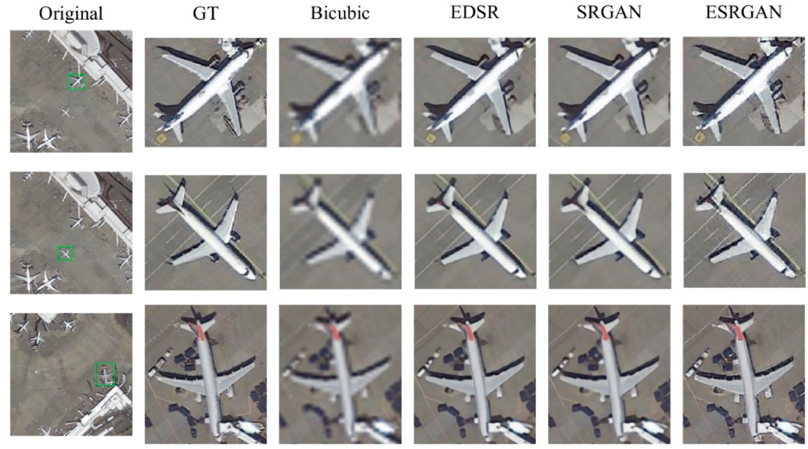
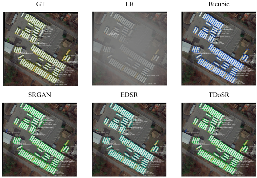
4.2. Comparative Experiment

When training the super-resolution model in this article, the original high-resolution data set is first down-sampled, then these down-sampled images are artificially fogged, and finally a low-resolution remote sensing image data set under foggy conditions is obtained. The low-resolution data set and the original high-resolution data set are then input into the super-resolution network for training so to complete the reconstruction of a super-resolution remote sensing image. The reconstructed image is input into the trained detector, and the performance of the super-resolution reconstruction network is tested by the recognition rate of different categories.

PSNR [30] and SSIM [31,32] are general indicators for evaluating image quality in the field of image processing, and are used in this paper. The detailed calculation formula and description are as follows:

PSNR is the most common and widely used image objective evaluation index. It is based on the error between corresponding pixels, that is, based on the error-sensitive image quality evaluation. It is calculated as follows:

$$\begin{array}{c}MSE=\frac{1}{H\times W}{\displaystyle \sum _{i=1}^H{\displaystyle \sum _{j=1}^W{(X(i,j)-Y(i,j))}^2}};\\ PSNR=10{\log }_{10}\left(\frac{{\left(2^n-1\right)}^2}{MSE}\right)\end{array}$$

(15)

where MSE represents the mean square error of the current image X and the reference image Y, $X\left(i,j\right)$ and $Y\left(i,j\right)$ represent the pixel values at the corresponding coordinates, H and W are the height and width of the image, respectively, and n is the number of bits per pixel (generally 8). The unit of PSNR is dB. The larger the value, the smaller the distortion, because larger values indicate a smaller MSE. If the MSE is smaller, and if the two images are closer, then the distortion is also smaller.

SSIM is structural similarity, which is an index to measure the similarity of two images. The calculation formula of SSIM is as follows:

$$\begin{array}{c}L(X,Y)=\frac{2u_X{u}_Y+C_1}{u_X^2+u_Y^2+C_1};\\ C(X,Y)=\frac{2{\sigma }_X{\sigma }_Y+C_2}{{\sigma }_X^2+{\sigma }_Y^2+C_2};\\ S(X,Y)=\frac{{\sigma }_{XY}+C_3}{{\sigma }_X{\sigma }_Y+C_3};\\ SSIM(X,Y)=L\left(X,Y\right)·C\left(X,Y\right)·S\left(X,Y\right)\end{array}$$

(16)

where $u_X$ and $u_Y$ represent the mean values of images X and Y, respectively; ${\sigma }_X$ and ${\sigma }_Y$ represent the standard deviations of images X and Y, respectively; ${\sigma }_X^2$, ${\sigma }_Y^2$ represent the variances of images X and Y, respectively; and ${\sigma }_{XY}$ represents the covariances of images X and Y. $C_1,C_2,C_3$ is a constant and usually takes $C_1={\left(K_{1}L\right)}^2$, $C_2={\left(K_{2}L\right)}^2$, $C_3=\frac{C_2}{2}$, and generally $K_1=0.01,K_2=0.03,L=255$.

The image after super-resolution reconstruction is shown in Figure 4. The reconstruction effect of the ESRGAN algorithm is the best, and the reconstructed image is closest to the original image. The average values of the objective evaluation indexes PSNR and SSIM after the super-resolution reconstruction of the various algorithms are calculated on the test set, as listed in

Table 1. Comparison of the objective evaluation indicators of different super-resolution methods.

Method	PSNR	SSIM
Bicubic	28.3841	0.7345
SRGAN	36.3838	0.8830
EDSR	36.4970	0.8841
ESRGAN	36.5556	0.8846

. After comparison, the traditional interpolation algorithm has the worst effect, and the ESRGAN algorithm selected for this paper not only achieves the best objective evaluation index, but also shows the superiority of this algorithm in sensory vision.

4.3. Results and Analysis

The unprocessed original real high-definition image is input into the detector model for testing, and the recognition accuracy of different categories in the original image is obtained, as shown in

Table 2. The recognition accuracy of various targets after the reconstruction by different super-resolution methods.

Method	PL	BD	BR	GTF	SV	LV	SH	TC	BC	ST	SBF	RA	HA	SP	HC	CC
GT	88.51	86.45	61.23	81.20	67.60	83.65	90.00	90.86	84.30	75.33	71.49	72.06	78.32	74.73	76.10	46.98
LR	67.89	66.93	42.01	61.33	47.72	63.74	70.12	71.05	64.41	55.56	51.62	52.17	58.29	54.68	56.67	15.33
Bicubic	78.37	77.65	52.40	72.43	59.71	74.73	81.72	82.34	75.60	66.71	63.12	64.01	70.03	65.28	67.91	23.47
SRGAN	84.39	82.57	57.61	77.51	63.59	79.82	86.21	86.72	80.39	71.42	67.53	68.11	74.51	70.82	72.33	39.56
EDSR	85.60	84.71	59.90	78.72	65.32	81.03	87.08	88.11	81.89	72.35	68.79	69.02	75.84	72.31	74.87	41.64
TDoSR (Our)	87.63	85.37	60.12	80.01	66.72	82.59	88.97	89.43	83.18	74.36	70.38	70.98	77.29	73.82	75.13	45.03

. The trained model of the detector selected in this paper has better performance and recognition ability.

In the experiment of super-resolution reconstruction, three algorithms (Bicubic, SRGAN, and EDSR) are selected for comparison with the ESRGAN algorithm used in this paper. Among them, the Bicubic algorithm uses traditional interpolation methods to complete the image super-resolution work. The SRGAN algorithm is the first method to apply the GAN to the super-resolution deep learning. The EDSR algorithm is improved based on the SRGAN network. The ESRGAN algorithm is the best way to deal with the super-resolution reconstruction of remote sensing images.

The super-resolution images reconstructed by different algorithms are input into the detector model for classification and recognition, respectively, whereby the recognition rate of each category is obtained. The recognition accuracy of each category is counted and sorted, as shown in Table 2. The actual recognition effect is shown in Figure 5. In Table 2, the horizontal row represents the recognition rate of each type of target, and the vertical row represents the different super-resolution methods, where GT is the real image and LR is the real image which is fogged after the image down-sampling.

It may be concluded from the recognition accuracy of Table 2 that the recognition effect is the best in the original high-definition image, while the traditional Bicubic interpolation algorithm has the worst effect, with a 10% decline when compared to the original image. No additional effective information was introduced in the process, the reconstruction effect was poor, and the recognition rate was also the lowest. While several other deep learning-based super-resolution algorithms rebuild images and improve the image resolution, they also introduce external information for the image reconstruction so that the images have more detailed information. The ESRGAN algorithm selected for this paper has the best performance in terms of both visual effects and objective evaluation indicators. The reconstructed remote sensing image has rich texture details, the edge information is more obvious, and the recognition rate is the highest among all the algorithms. The accuracy difference is only roughly 1.2%.

The remote sensing image recognition algorithm proposed in this paper effectively solves the problem of the low recognition rate of low-resolution remote sensing images in foggy scenes.

5. Discussion

This paper proposed a new method for target detection in low-resolution remote sensing images in foggy weather. The low-resolution foggy remote sensing image was super-resolution reconstructed via the ESRGAN network, and the reconstructed super-resolution image was input to the recognition classification in the trained detector model. After many experiments, this method improved the target recognition rate of low-resolution remote sensing images by nearly 20%. The main contributions of this paper are as follows. First, the application of image super-resolution reconstruction technology to the task of target detection in remote sensing images has broadened the application range of image super-resolution reconstruction technology. Furthermore, this research has realized the recognition and detection of small and weak targets on low-resolution remote sensing images under foggy conditions and achieved a very good detection effect. Finally, this paper compared the different methods of image super-resolution reconstruction at this stage, and ultimately selected the ESRGAN method as the best through many experiments, which helps the target detection task of remote sensing images at low resolution. The research undertaken in this paper has some benefit to the application of super-resolution reconstruction technology in the field of target detection. In the past two years, Transformer has shown the advantages in processing computer vision tasks, and has provided new research directions for the future of for the super-resolution reconstruction of remote sensing images.

References

1. Steve, L.; Giles, C.L.; Tsoi, A.C.; Back, A.D. Face Recognition: A Convolutional Neural-Network Approach. IEEE Trans. Neural Netw. 1997, 8, 98–113. [Google Scholar]
2. Claus, N. Evaluation of Convolutional Neural Networks for Visual Recognition. IEEE Trans. Neural Netw. 1998, 9, 685–696. [Google Scholar]
3. Christian, S.; Liu, W.; Jia, Y.; Sermanet, P.; Reed, S.E.; Anguelov, D.; Erhan, D.; Vanhoucke, V.; Rabinovich, A. Going Deeper with Convolutions. In Proceedings of the IEEE Conference on Computer Vision and Pattern Recognition, CVPR 2015, Boston, MA, USA, 7–12 June 2015. [Google Scholar]
4. Chao, D.; Loy, C.C.; He, K.; Tang, X. Part IV—Learning a Deep Convolutional Network for Image Super-Resolution. In Proceedings of the Computer Vision—ECCV 2014—13th European Conference, Zurich, Switzerland, 6–12 September 2014. [Google Scholar]
5. He, K.; Zhang, X.; Ren, S.; Sun, J. Deep Residual Learning for Image Recognition. In Proceedings of the 2016 IEEE Conference on Computer Vision and Pattern Recognition, CVPR 2016, Las Vegas, NV, USA, 27–30 June 2016. [Google Scholar]
6. Shi, W.; Caballero, J.; Huszár, F.; Totz, J.; Aitken, A.P.; Bishop, R.; Rueckert, D.; Wang, Z. Real-Time Single Image and Video Super-Resolution Using an Efficient Sub-Pixel Convolutional Neural Network. In Proceedings of the 2016 IEEE Conference on Computer Vision and Pattern Recognition, CVPR 2016, Las Vegas, NV, USA, 27–30 June 2016. [Google Scholar]
7. Christian, L.; Theis, L.; Huszar, F.; Caballero, J.; Cunningham, A.; Acosta, A.; Aitken, A.P.; Tejani, A.; Totz, J.; Wang, Z.; et al. Photo-Realistic Single Image Super-Resolution Using a Generative Adversarial Network. In Proceedings of the 2017 IEEE Conference on Computer Vision and Pattern Recognition, CVPR 2017, Honolulu, HI, USA, 21–26 July 2017. [Google Scholar]
8. Ian, J.G.; Abadie, J.P.; Mirza, M.; Xu, B.; WardeFarley, D.; Ozair, S.; Courville, A.C.; Bengio, Y. Generative Adversarial Networks. Commun. ACM 2020, 63, 139–144. [Google Scholar]
9. Kim, J.; Lee, J.K.; Lee, K.M. Accurate Image Super-Resolution Using Very Deep Convolutional Networks. In Proceedings of the 2016 IEEE Conference on Computer Vision and Pattern Recognition, CVPR 2016, Las Vegas, NV, USA, 27–30 June 2016. [Google Scholar]
10. Sergey, I.; Szegedy, C. Batch Normalization: Accelerating Deep Network Training by Reducing Internal Covariate Shift. In Proceedings of the 32nd International Conference on Machine Learning, ICML 2015, Lille, France, 6–11 July 2015. [Google Scholar]
11. He, K.; Zhang, X.; Ren, S.; Sun, J. Delving Deep into Rectifiers: Surpassing Human-Level Performance on Imagenet Classification. In Proceedings of the 2015 IEEE International Conference on Computer Vision, ICCV 2015, Santiago, Chile, 7–13 December 2015. [Google Scholar]
12. Bee, L.; Son, S.; Kim, H.; Nah, S.; Lee, K.M. Enhanced Deep Residual Networks for Single Image Super-Resolution. In Proceedings of the 2017 IEEE Conference on Computer Vision and Pattern Recognition Workshops, CVPR Workshops 2017, Honolulu, HI, USA, 21–26 July 2017. [Google Scholar]
13. Wang, X.; Yu, K.; Wu, S.; Gu, J.; Liu, Y.; Dong, C.; Qiao, Y.; Change Loy, C. Part V—Esrgan: Enhanced Super-Resolution Generative Adversarial Networks. In Proceedings of the Computer Vision—ECCV 2018 Workshops, Munich, Germany, 8–14 September 2018. [Google Scholar]
14. Karen, S.; Zisserman, A. Very Deep Convolutional Networks for Large-Scale Image Recognition. In Proceedings of the 3rd International Conference on Learning Representations, ICLR 2015, San Diego, CA, USA, 7–9 May 2015. [Google Scholar]
15. Kwan, C.; Dao, M.; Chou, B.; Kwan, L.M.; Ayhan, B. Mastcam Image Enhancement Using Estimated Point Spread Functions. In Proceedings of the 8th IEEE Annual Ubiquitous Computing, Electronics and Mobile Communication Conference, UEMCON, New York, NY, USA, 19–21 October 2017. [Google Scholar]
16. Han, J.; Ding, J.; Xue, N.; Xia, G.S. Redet: A Rotation-Equivariant Detector for Aerial Object Detection. In Proceedings of the IEEE Conference on Computer Vision and Pattern Recognition, CVPR 2021, Nashville, TN, USA, 19–25 June 2021. [Google Scholar]
17. Jian, D.; Xue, N.; Long, Y.; Xia, G.; Lu, Q. Learning Roi Transformer for Oriented Object Detection in Aerial Images. In Proceedings of the IEEE Conference on Computer Vision and Pattern Recognition, CVPR 2019, Long Beach, CA, USA, 16–20 June 2019. [Google Scholar]
18. Xue, Y.; Yan, J. Part VIII—Arbitrary-Oriented Object Detection with Circular Smooth Label. In Proceedings of the Computer Vision—ECCV 2020—16th European Conference, Glasgow, UK, 23–28 August 2020. [Google Scholar]
19. Ma, J.; Shao, W.; Ye, H.; Wang, L.; Wang, H.; Zheng, Y.; Xue, X. Arbitrary-Oriented Scene Text Detection via Rotation Proposals. IEEE Trans. Multimed. 2018, 20, 3111–3122. [Google Scholar]
20. Xia, G.S.; Bai, X.; Ding, J.; Zhu, Z.; Belongie, S.; Luo, J.; Datcu, M.; Pelillo, M.; Zhang, L. Dota: A Large-Scale Dataset for Object Detection in Aerial Images. In Proceedings of the 2018 IEEE Conference on Computer Vision and Pattern Recognition, CVPR 2018, Salt Lake City, UT, USA, 18–22 June 2018. [Google Scholar]
21. Chao, D.; Loy, C.C.; He, K.; Tang, X. Image Super-Resolution Using Deep Convolutional Networks. IEEE Trans. Pattern Anal. Mach. Intell. 2015, 38, 295–307. [Google Scholar]
22. Joan, B.; Sprechmann, P.; LeCun, Y. Super-Resolution with Deep Convolutional Sufficient Statistics. In Proceedings of the 4th International Conference on Learning Representations, ICLR 2016, San Juan, PR, USA, 2–4 May 2016. [Google Scholar]
23. Justin, J.; Alahi, A.; FeiFei, L. Part II—Perceptual Losses for Real-Time Style Transfer and Super-Resolution. In Proceedings of the Computer Vision—ECCV 2016—14th European Conference, Amsterdam, The Netherlands, 11–14 October 2016. [Google Scholar]
24. Alec, R.; Metz, L.; Chintala, S. Unsupervised Representation Learning with Deep Convolutional Generative Adversarial Networks. In Proceedings of the 4th International Conference on Learning Representations, ICLR 2016, San Juan, PR, USA, 2–4 May 2016. [Google Scholar]
25. Lai, W.S.; Huang, J.B.; Ahuja, N.; Yang, M.H. Deep Laplacian Pyramid Networks for Fast and Accurate Super-Resolution. In Proceedings of the 2017 IEEE Conference on Computer Vision and Pattern Recognition, CVPR 2017, Honolulu, HI, USA, 21–26 July 2017. [Google Scholar]
26. Christian, S.; Ioffe, S.; Vanhoucke, V.; Alemi, A.A. Inception-V4, Inception-Resnet and the Impact of Residual Connections on Learning. In Proceedings of the Thirty-First AAAI Conference on Artificial Intelligence, San Francisco, CA, USA, 4–9 February 2017. [Google Scholar]
27. TsungYi, L.; Dollr, P.; Girshick, R.B.; He, K.; Hariharan, B.; Belongie, S.J. Feature Pyramid Networks for Object Detection. In Proceedings of the 2017 IEEE Conference on Computer Vision and Pattern Recognition, CVPR 2017, Honolulu, HI, USA, 21–26 July 2017. [Google Scholar]
28. Ren, S.; He, K.; Girshick, R.B.; Sun, J. Faster R-Cnn: Towards Real-Time Object Detection with Region Proposal Networks. IEEE Trans. Pattern Anal. Mach. Intell. 2017, 39, 1137–1149. [Google Scholar]
29. Diederik, P.K.; Ba, J. Adam: A Method for Stochastic Optimization. In Proceedings of the 3rd International Conference on Learning Representations, ICLR 2015, San Diego, CA, USA, 7–9 May 2015. [Google Scholar]
30. Adam, P.; Gross, S.; Massa, F.; Lerer, A.; Bradbury, J.; Chanan, G.; Killeen, T.; Lin, Z.; Gimelshein, N.; Antiga, L.; et al. Pytorch: An Imperative Style, High-Performance Deep Learning Library. In Proceedings of the Advances in Neural Information Processing Systems 32: Annual Conference on Neural Information Processing Systems 2019, NeurIPS 2019, Vancouver, BC, Canada, 8–14 December 2019. [Google Scholar]
31. Kai, C.; Wang, J.; Pang, J.; Cao, Y.; Xiong, Y.; Li, X.; Sun, S.; Feng, W.; Liu, Z.; Xu, J.; et al. Mmdetection: Open Mmlab Detection Toolbox and Benchmark. arXiv 2019, arXiv:1906.07155. [Google Scholar]
32. Ying, T.; Yang, J.; Liu, X. Image Super-Resolution via Deep Recursive Residual Network. In Proceedings of the 2017 IEEE Conference on Computer Vision and Pattern Recognition, CVPR 2017, Honolulu, HI, USA, 21–26 July 2017. [Google Scholar]
Figure 1. (a) Interpolation basis function diagram; (b) Schematic diagram of the bicubic algorithm.
Photonics 08 00431 g001
Figure 2. (a) The image after down-sampling; (b) the fogged image after down-sampling.
Photonics 08 00431 g002
Figure 3. A flow chart of the remote sensing image recognition algorithm. Down-sampling the real high-definition image to obtain a low-resolution image, then simulating the fogging process on the low-resolution image to obtain a low-resolution foggy image, which is then super-resolution reconstructed, and finally the reconstructed image Target recognition on the image.
Photonics 08 00431 g003
Figure 4. Comparison of the results of different super-resolution methods.
Photonics 08 00431 g004
Figure 5. Recognition effect diagram of different methods.
Photonics 08 00431 g005