Comparative Modeling of Infrared Fiber Lasers

 , ,
, ,  , ,
, ,  and
and
Abstract
1. Introduction
2. Materials and Methods
- The fiber laser model developed at the Institute of Photonics and Electronics of the Czech Academy of Sciences (UFE) was implemented in C programming language (gcc 4.9.2) within the Windows 7 operating system, 64 bit Intel core i7-3930K CPU at 3.2 GHz. The UFE model is currently being developed for the study of longitudinal-mode instabilities and associated buildup of dynamic fiber Bragg gratings [40].
- The fiber laser model developed at the Politecnico di Bari (PB) was implemented in MATLAB within the Windows 10 operating system, 64-bit Intel Core i7-4790 CPU at 3.6 GHz. The numerical integration was carried out using a 4-5 Runge–Kutta algorithm, and the more rigorous overlap integrals approach was employed.
- The fiber laser model developed at the University of Nottingham and Wroclaw University of Science and Technology (NU–PWr) was implemented in MATLAB within the Windows 10 operating system, 64 bit Intel Core i5 7th Generation, CPU at 2.5 GHz. The numerical integration was carried out using a 4-5 Runge–Kutta algorithm.
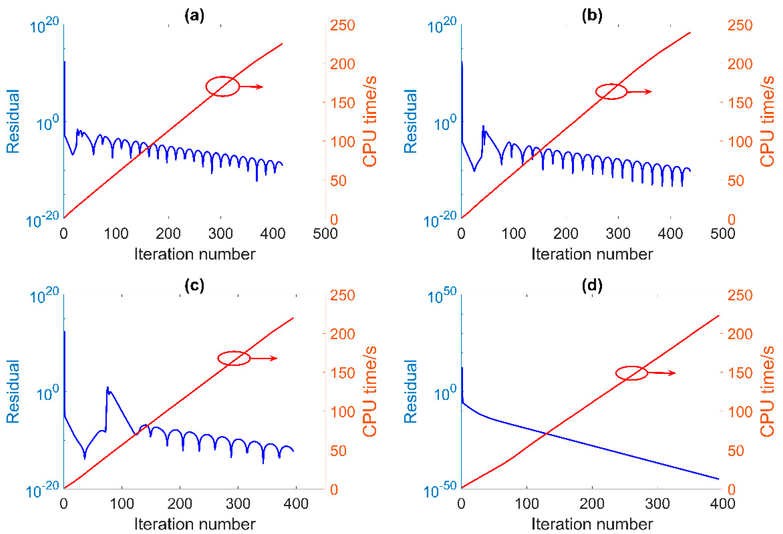
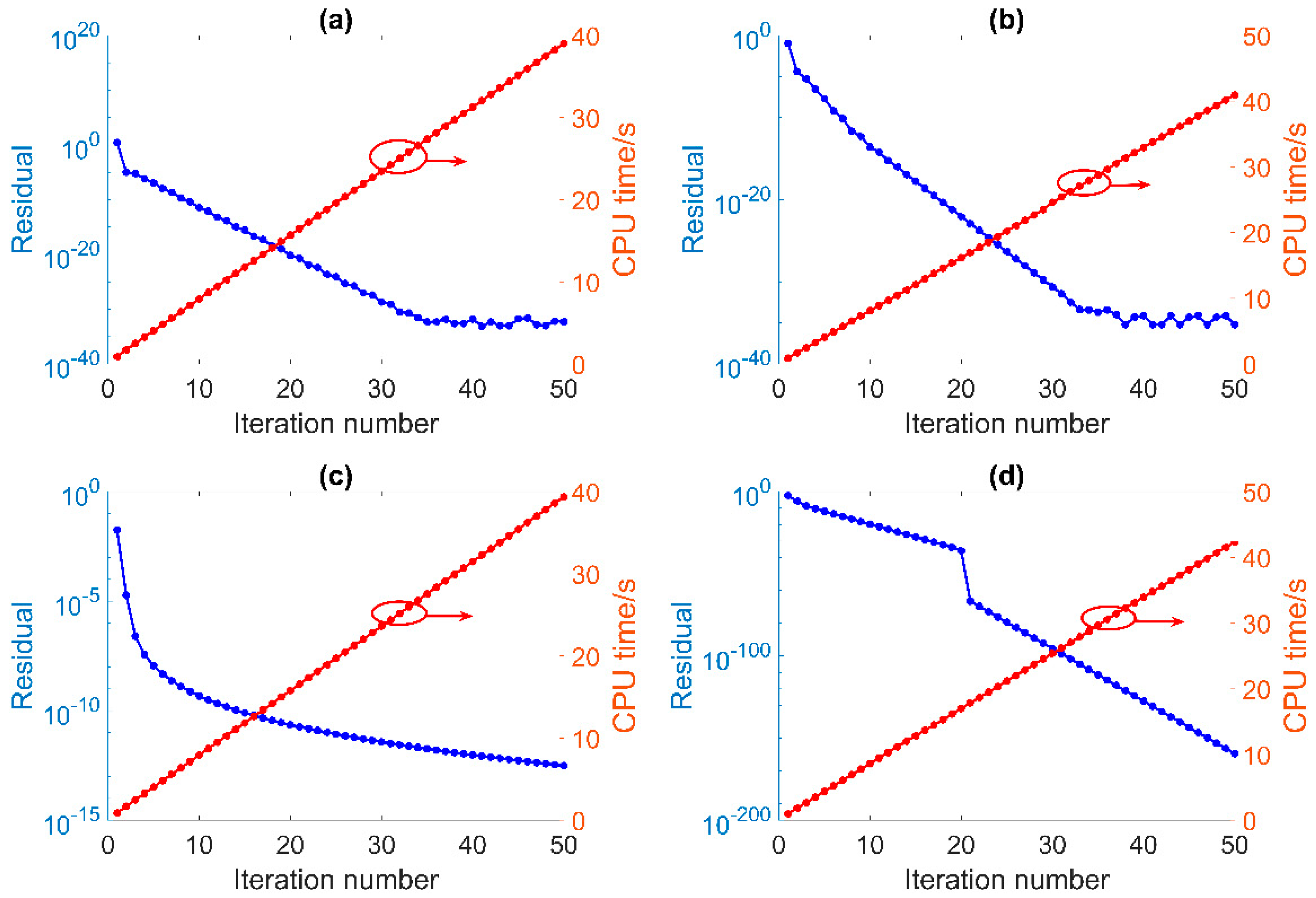
3. Results
4. Conclusions
Author Contributions
Funding
Acknowledgments
Conflicts of Interest
References
- Schneider, J.; Carbonnier, C.; Unrau, U.B. Characterization of a Ho3+-doped fluoride fiber laser with a 3.9-mm emission wavelength. Appl. Opt. 1997, 36, 8595–8600. [Google Scholar] [CrossRef] [PubMed]
- Majewski, M.R.; Woodward, R.I.; Carreé, J.-Y.; Poulain, S.; Poulain, M.; Jackson, S.D. Emission beyond 4 μm and mid-infrared lasing in a dysprosium-doped indium fluoride InF3 fiber. Opt. Lett. 2018, 43, 1926–1929. [Google Scholar] [CrossRef] [PubMed]
- Maes, F.; Fortin, V.; Poulain, S.; Poulain, M.; Carrée, J.-Y.; Bernier, M.; Vallée, R. Room temperature fiber laser at 3.92 mm. arXiv 2018, arXiv:1804.08610. [Google Scholar]
- Písařík, M.; Peterka, P.; Aubrecht, J.; Cajzl, J.; Benda, A.; Mareš, D.; Todorov, F.; Podrazký, O.; Honzátko, P.; Kašík, I. Thulium-doped fibre broadband source for spectral region near 2 micrometers. Opto-Electron. Rev. 2016, 24, 223–231. [Google Scholar] [CrossRef]
- Tokita, S.; Murakami, M.; Shimizu, S.; Hashida, M.; Sakabe, S. Liquid-cooled 24 W mid-infrared Er:ZBLAN fiber laser. Opt. Lett. 2009, 34, 3062–3064. [Google Scholar] [CrossRef] [PubMed]
- Henderson-Sapir, O.; Jackson, S.D.; Ottaway, D.J. Versatile and widely tunable mid-infrared erbium doped ZBLAN fiber laser. Opt. Lett. 2016, 41, 1676–1679. [Google Scholar] [CrossRef] [PubMed]
- Henderson-Sapir, O.; Malouf, A.; Bawden, N.; Munch, J.; Jackson, S.D.; Ottaway, D.J. Recent Advances in 3.5 mm Erbium-Doped Mid-Infrared Fiber Lasers. IEEE J. Sel. Top. Quantum Electron. 2017, 23, 6–14. [Google Scholar] [CrossRef]
- Henderson-Sapir, O.; Munch, J.; Ottaway, D.J. New energy-transfer upconversion process in Er3+: ZBLAN mid-infrared fiber lasers. Opt. Express 2016, 24, 6869–6883. [Google Scholar] [CrossRef] [PubMed]
- Malouf, A.; Henderson-Sapir, O.; Gorjan, M.; Ottaway, D.J. Numerical Modeling of 3.5 mm Dual-Wavelength Pumped Erbium-Doped Mid-Infrared Fiber Lasers. IEEE J. Quantum Electron. 2016, 52, 1600412. [Google Scholar] [CrossRef]
- Lamrini, S.; Scholle, K.; Schäfer, M.; Fuhrberg, P.; Ward, J.; Francis, M.; Sujecki, S.; Oladeji, A.; Napier, B.; Seddon, A.B.; et al. High-Energy Q-switched Er:ZBLAN Fibre Laser at 2.79 mm. In Proceedings of the CLEO/Europe-EQEC OSA, Munich, Germany, 21–25 June 2015. [Google Scholar]
- Li, J.F.; Jackson, S.D. Numerical Modeling and Optimization of Diode Pumped Heavily-Erbium-Doped Fluoride Fiber Lasers. IEEE J. Quantum Electron. 2012, 48, 454–464. [Google Scholar] [CrossRef]
- Majewski, M.R.; Jackson, S.D. Highly efficient mid-infrared dysprosium fiber laser. Opt. Lett. 2016, 41, 2173–2176. [Google Scholar] [CrossRef] [PubMed]
- Sakr, H.; Furniss, D.; Tang, Z.; Sojka, L.; Moneim, N.A.; Barney, E.; Sujecki, S.; Benson, T.M.; Seddon, A.B. Superior photoluminescence (PL) of Pr3+-In, compared to Pr3+-Ga, selenide-chalcogenide bulk glasses and PL of optically-clad fiber. Opt. Express 2014, 22, 21236–21252. [Google Scholar] [CrossRef] [PubMed]
- Sakr, H.; Tang, Z.Q.; Furniss, D.; Sojka, L.; Sujecki, S.; Benson, T.M.; Seddon, A.B. Promising emission behavior in Pr3+/In selenide-chalcogenide-glass small-core step index fiber (SIF). Opt. Mater. 2017, 67, 98–107. [Google Scholar] [CrossRef]
- Seddon, A.B.; Furniss, D.; Tang, Z.Q.; Sojka, L.; Benson, T.M.; Caspary, R.; Sujecki, S. True Mid-Infrared Pr3+ Absorption Cross-Section in a Selenide-Chalcogenide Host-Glass. In Proceedings of the 2016 18th International Conference on Transparent Optical Networks, Trento, Italy, 10–14 July 2016. [Google Scholar]
- Seddon, A.B.; Tang, Z.; Furniss, D.; Sujecki, S.; Benson, T.M. Progress in rare-earth-doped mid-infrared fiber lasers. Opt. Express 2010, 18, 26704–26719. [Google Scholar] [CrossRef] [PubMed]
- Sojka, L.; Tang, Z.; Furniss, D.; Sakr, H.; Beres-Pawlik, E.; Seddon, A.B.; Benson, T.M.; Sujecki, S. Numerical and experimental investigation of mid-infrared laser action in resonantly pumped Pr3+ doped chalcogenide fibre. Opt. Quantum Electron. 2017, 49, 21. [Google Scholar] [CrossRef]
- Sojka, L.; Tang, Z.; Furniss, D.; Sakr, H.; Fang, Y.; Beres-Pawlik, E.; Benson, T.M.; Seddon, A.B.; Sujecki, S. Mid-infrared emission in Tb3+-doped selenide glass fiber. J. Opt. Soc. Am. B Opt. Phys. 2017, 34, A70–A79. [Google Scholar] [CrossRef]
- Sojka, L.; Tang, Z.; Furniss, D.; Sakr, H.; Oladeji, A.; Beres-Pawlik, E.; Dantanarayana, H.; Faber, E.; Seddon, A.B.; Benson, T.M.; et al. Broadband, mid-infrared emission from Pr3+ doped GeAsGaSe chalcogenide fiber, optically clad. Opt. Mater. 2014, 36, 1076–1082. [Google Scholar] [CrossRef]
- Sojka, L.; Tang, Z.; Zhu, H.; Beres-Pawlik, E.; Furniss, D.; Seddon, A.B.; Benson, T.M.; Sujecki, S. Study of mid-infrared laser action in chalcogenide rare earth doped glass with Dy3+, Pr3+ and Tb3+. Opt. Mater. Express 2012, 2, 1632–1640. [Google Scholar] [CrossRef]
- Tang, Z.; Furniss, D.; Fay, M.; Sakr, H.; Sojka, L.; Neate, N.; Weston, N.; Sujecki, S.; Benson, T.M.; Seddon, A.B. Mid-infrared photoluminescence in small-core fiber of praseodymium-ion doped selenide-based chalcogenide glass. Opt. Mater. Express 2015, 5, 870–886. [Google Scholar] [CrossRef]
- Tang, Z.; Neate, N.C.; Furniss, D.; Sujecki, S.; Benson, T.M.; Seddon, A.B. Crystallization behavior of Dy3+-doped selenide glasses. J. Non-Cryst. Solids 2011, 357, 2453–2462. [Google Scholar] [CrossRef]
- Tang, Z.Q.; Shiryaev, V.S.; Furniss, D.; Sojka, L.; Sujecki, S.; Benson, T.M.; Seddon, A.B.; Churbanov, M.F. Low loss Ge-As-Se chalcogenide glass fiber, fabricated using extruded preform, for mid-infrared photonics. Opt. Mater. Express 2015, 5, 1722–1737. [Google Scholar] [CrossRef]
- Churbanov, M.F.; Scripachev, I.V.; Shiryaev, V.S.; Plotnichenko, V.G.; Smetanin, S.V.; Kryukova, E.B.; Pyrkov, Y.N.; Galagan, B.I. Chalcogenide glasses doped with Tb, Dy and Pr ions. J. Non-Cryst. Solids 2003, 326, 301–305. [Google Scholar] [CrossRef]
- Karaksina, E.V.; Shiryaev, V.S.; Churbanov, M.F.; Anashkina, E.A.; Kotereva, T.V.; Snopatin, G.E. Core-clad Pr3+-doped Ga(In)-Ge-As-Se-(I) glass fibers: Preparation, investigation, simulation of laser characteristics. Opt. Mater. 2017, 72, 654–660. [Google Scholar] [CrossRef]
- Karaksina, E.V.; Shiryaev, V.S.; Kotereva, T.V.; Churbanov, M.F. Preparation of high-purity Pr3+ doped Ge-Ga-Sb-Se glasses with intensive middle infrared luminescence. J. Lumin. 2016, 170, 37–41. [Google Scholar] [CrossRef]
- Shiryaev, V.S.; Karaksina, E.V.; Kotereva, T.V.; Churbanov, M.F.; Velmuzhov, A.P.; Sukhanov, M.V.; Ketkova, L.A.; Zernova, N.S.; Plotnichenko, V.G.; Koltashev, V.V. Preparation and investigation of Pr3+-doped Ge-Sb-Se-In-I glasses as promising material for active mid-infrared optics. J. Lumin. 2017, 183, 129–134. [Google Scholar] [CrossRef]
- Quimby, R.S.; Shaw, L.B.; Sanghera, J.S.; Aggarwal, I.D. Modeling of cascade lasing in Dy: Chalcogenide glass fiber laser with efficient output at 4.5 mm. IEEE Photonics Technol. Lett. 2008, 20, 123–125. [Google Scholar] [CrossRef]
- Sanghera, J.S.; Shaw, L.B.; Aggarwal, I.D. Chalcogenide Glass-Fiber-Based Mid-IR Sources and Applications. IEEE J. Sel. Top. Quantum Electron. 2009, 15, 114–119. [Google Scholar] [CrossRef]
- Shaw, L.B.; Cole, B.; Thielen, P.A.; Sanghera, J.S.; Aggarwal, I.D. Mid-wave IR and long-wave IR laser potential of rare-earth doped chalcogenide glass fiber. IEEE J. Quantum Electron. 2001, 37, 1127–1137. [Google Scholar] [CrossRef]
- Falconi, M.C.; Palma, G.; Starecki, F.; Nazabal, V.; Troles, J.; Adam, J.L.; Taccheo, S.; Ferrari, M.; Prudenzano, F. Dysprosium-Doped Chalcogenide Master Oscillator Power Amplifier (MOPA) for Mid-IR Emission. J. Light. Technol. 2017, 35, 265–273. [Google Scholar] [CrossRef]
- Falconi, M.C.; Palma, G.; Starecki, F.; Nazabal, V.; Troles, J.; Taccheo, S.; Ferrari, M.; Prudenzano, F. Design of an Efficient Pumping Scheme for Mid-IR Dy3+:Ga5Ge20Sb10S65 PCF Fiber Laser. IEEE Photonics Technol. Lett. 2016, 28, 1984–1987. [Google Scholar] [CrossRef]
- Moizan, V.; Nazabal, V.; Troles, J.; Houizot, P.; Adam, J.-L.; Doualan, J.-L.; Moncorge, R.; Smektala, F.; Gadret, G.; Pitois, S.; et al. Er3+-doped GeGaSbS glasses for mid-IR fibre laser application: Synthesis and rare earth spectroscopy. Opt. Mater. 2008, 31, 39–46. [Google Scholar] [CrossRef]
- Pele, A.L.; Braud, A.; Doualan, J.L.; Starecki, F.; Nazabal, V.; Chahal, R.; Boussard-Pledel, C.; Bureau, B.; Moncorge, R.; Camy, P. Dy3+ doped GeGaSbS fluorescent fiber at 4.4 mm for optical gas sensing: Comparison of simulation and experiment. Opt. Mater. 2016, 61, 37–44. [Google Scholar] [CrossRef]
- Starecki, F.; Morais, S.; Chahal, R.; Boussard-Pledel, C.; Bureau, B.; Palencia, F.; Lecoutre, C.; Garrabos, Y.; Marre, S.; Nazabal, V. IR emitting Dy3+ doped chalcogenide fibers for in situ CO2 monitoring in high pressure microsystems. Int. J. Greenh. Gas Control 2016, 55, 36–41. [Google Scholar] [CrossRef]
- Sujecki, S. An Efficient Algorithm for Steady State Analysis of Fibre Lasers Operating under Cascade Pumping Scheme. Int. J. Electron. Telecommun. 2014, 60, 143–149. [Google Scholar] [CrossRef]
- Sujecki, S. Numerical Analysis of Q-Switched Erbium Ion Doped Fluoride Glass Fiber Laser Operation Including Spontaneous Emission. Appl. Sci. 2018, 8, 803. [Google Scholar] [CrossRef]
- Sujecki, S.; Sojka, L.; Beres-Pawlik, E.; Tang, Z.; Furniss, D.; Seddon, A.B.; Benson, T.M. Modelling of a simple Dy3+ doped chalcogenide glass fibre laser for mid-infrared light generation. Opt. Quantum Electron. 2010, 42, 69–79. [Google Scholar] [CrossRef]
- Falconi, M.C.; Palma, G.; Starecki, F.; Nazabal, V.; Troles, J.; Adam, J.L.; Taccheo, S.; Ferrari, M.; Prudenzano, F. Novel Pumping Schemes of Mid-IR Photonic Crystal Fiber Lasers for Aerospace Applications. In Proceedings of the 2016 18th International Conference on Transparent Optical Networks, Trento, Italy, 10–14 July 2016. [Google Scholar]
- Peterka, P.; Koška, P.; Čtyroký, J. Reflectivity of superimposed Bragg gratings induced by longitudinal mode instabilities in fiber lasers. IEEE J. Sel. Top. Quantum Electron. 2018, 24, 1–8. [Google Scholar] [CrossRef]
- Falconi, M.C.; Palma, G.; Starecki, F.; Nazabal, V.; Troles, J.; Adam, J.L.; Taccheo, S.; Ferrari, M.; Prudenzano, F. Recent Advances on Pumping Schemes for Mid-IR PCF Lasers. In Optical Components and Materials XIV; Jiang, S., Digonnet, M.J.F., Eds.; SPIE: Bellingham, WA, USA, 2017; Volume 10100. [Google Scholar]
- Khamis, M.A.; Sevilla, R.; Ennser, K. Large Mode Area Pr3+-Doped Chalcogenide PCF Design for High Efficiency Mid-IR Laser. IEEE Photonics Technol. Lett. 2018, 30, 825–828. [Google Scholar] [CrossRef]
- Hu, J.; Menyuk, C.R.; Wei, C.L.; Shaw, L.B.; Sanghera, J.S.; Aggarwal, I.D. Highly efficient cascaded amplification using Pr3+-doped mid-infrared chalcogenide fiber amplifiers. Opt. Lett. 2015, 40, 3687–3690. [Google Scholar] [CrossRef] [PubMed]
- Anashkina, E.A. Design and Numerical Modeling of Broadband Mid-IR Rare-Earth-Doped Chalcogenide Fiber Amplifiers. IEEE Photonics Technol. Lett. 2018, 30, 1190–1193. [Google Scholar] [CrossRef]
- Falconi, M.C.; Bozzetti, M.; Fernandez, T.; Galzerano, G.; Prudenzano, F. Design of an Efficient Pulsed Dy3+: ZBLAN Fiber Laser Operating in Gain Switching Regime. J. Light. Technol. 2018, 36, 5327–5331. [Google Scholar] [CrossRef]


| Quantity | Unit | Value |
|---|---|---|
| Dy3+ ion concentration NDy | cm−3 | 7 × 10¹⁹ |
| Aeff | m2 | 95 × 10−12 |
| Fiber length L | m | 2.1 |
| Fiber loss at all wavelengths α | dB/m | 1 |
| Lifetime of level 2 (Figure 2) | ms | 2 |
| Lifetime of level 1 (Figure 2) | ms | 5.2 |
| Branching ratio for 2-1 transitions | 0.15 | |
| Reflectivity for idler, signal, and pump at z = 0 | 0.2 | |
| Reflectivity for idler, signal, and pump at z = L | 0.2 | |
| Confinement factor for signal | 0.8 | |
| Confinement factor for idler | 0.9 | |
| Confinement factor for pump | 0.034 | |
| Pump wavelength | μm | 1.71 |
| Signal wavelength (λ1) | μm | 4.6 |
| Idler wavelength (λ2) | μm | 3.35 |
| Pump emission cross section | m2 | 0.318 × 10⁻²⁴ |
| Pump absorption cross section | m2 | 0.501 × 10⁻²⁴ |
| Signal emission cross section | m2 | 0.912 × 10⁻²⁴ |
| Signal absorption cross section | m2 | 0.485 × 10⁻²⁴ |
| Idler emission cross section | m2 | 0.097 × 10⁻²⁴ |
| Idler absorption cross section | m2 | 0.016 × 10⁻²⁴ |
| Quantity | Unit | Value |
|---|---|---|
| b1/b2 | 0.1/0.16 | |
| W11 | m3/s | 1 × 10⁻²⁴ |
| W22 | m3/s | 0.3 × 10⁻²⁴ |
| σGSA | m2 | 2.1 × 10⁻²⁵ |
| σSE | m2 | 4.5 × 10⁻²⁵ |
| σESA | m2 | 1.1 × 10⁻²⁵ |
| Γp | 0.009 | |
| Γs | 1.0 | |
| Er3+ ion concentration NEr | m−3 | 9.6 × 1026 |
| Pump wavelength λp | Nm | 976 |
| Pump wavelength λs | Nm | 2800 |
| Fiber length L | m | 2.5 |
| Aeff | m2 | 314 × 10−12 |
| αp | 1/m | 3 × 10⁻³ |
| αs | 1/m | 23 × 10−3 |
| Rp (z = 0) | 0 | |
| Rp (z = L) | 0.04 | |
| Rs (z = 0) | 0.96 | |
| Rs (z = L) | 0.04 |
| Quantity | Unit | Value |
|---|---|---|
| τ1 | ms | 9 |
| τ2 | ms | 6.9 |
| τ3 | ms | 0.12 |
| τ4 | ms | 0.57 |
| β21, β20 | 0.37, 0.63 | |
| β32, β31, β30 | 0.856, 0.004, 0.14 | |
| β43, β42, β41, β40 | 0.34, 0.04, 0.18, 0.44 |
| Pump Power/W | Signal Power (NU–PWr)/W | Signal Power (UFE)/W | Relative Difference |
|---|---|---|---|
| 0.2 | 4.733 × 10⁻³ | 4.731 × 10⁻³ | 0.422 × 10⁻³ |
| 0.4 | 8.744 × 10⁻³ | 8.736 × 10⁻³ | 0.915 × 10⁻³ |
| 1 | 49.13 × 10⁻³ | 49.04 × 10⁻³ | 1.833 × 10⁻³ |
| 5 | 319.1 × 10⁻³ | 318.6 × 10⁻³ | 1.568 × 10⁻³ |
| Pump Power/W | Idler Power (NU–PWr)/W | Idler Power (UFE)/W | Relative Difference |
|---|---|---|---|
| 0.2 W | 0 W | 4.140 × 10⁻⁶ | NA |
| 0.4 W | 0 W | 9.591 × 10⁻⁴ | NA |
| 1 W | 55.38 × 10⁻³ W | 55.26 × 10⁻³ | 2.169 × 10⁻³ |
| 5 W | 426.0 × 10⁻³ W | 425.4 × 10⁻³ | 1.409 × 10⁻³ |
| Pump Power | Signal Power (NU–PWr)/W | Signal Power (UFE)/W | Relative Difference |
|---|---|---|---|
| 5 W | 1.432 | 1.432 | 0 |
| 10 W | 3.171 | 3.171 | 0 |
| 15 W | 4.868 | 4.868 | 0 |
| 20 W | 6.458 | 6.458 | 0 |
© 2018 by the authors. Licensee MDPI, Basel, Switzerland. This article is an open access article distributed under the terms and conditions of the Creative Commons Attribution (CC BY) license (http://creativecommons.org/licenses/by/4.0/).
Share and Cite
Sujecki, S.; Sojka, L.; Seddon, A.B.; Benson, T.M.; Barney, E.; Falconi, M.C.; Prudenzano, F.; Marciniak, M.; Baghdasaryan, H.; Peterka, P.; et al. Comparative Modeling of Infrared Fiber Lasers. Photonics 2018, 5, 48. https://doi.org/10.3390/photonics5040048
Sujecki S, Sojka L, Seddon AB, Benson TM, Barney E, Falconi MC, Prudenzano F, Marciniak M, Baghdasaryan H, Peterka P, et al. Comparative Modeling of Infrared Fiber Lasers. Photonics. 2018; 5(4):48. https://doi.org/10.3390/photonics5040048
Chicago/Turabian StyleSujecki, Slawomir, Lukasz Sojka, Angela B. Seddon, Trevor M. Benson, Emma Barney, Mario C. Falconi, Francesco Prudenzano, Marian Marciniak, Hovik Baghdasaryan, Pavel Peterka, and et al. 2018. "Comparative Modeling of Infrared Fiber Lasers" Photonics 5, no. 4: 48. https://doi.org/10.3390/photonics5040048
APA StyleSujecki, S., Sojka, L., Seddon, A. B., Benson, T. M., Barney, E., Falconi, M. C., Prudenzano, F., Marciniak, M., Baghdasaryan, H., Peterka, P., & Taccheo, S. (2018). Comparative Modeling of Infrared Fiber Lasers. Photonics, 5(4), 48. https://doi.org/10.3390/photonics5040048