Article

High Throughput AOTF Hyperspectral Imager for Randomly Polarized Light

1
School of Biomedical Engineering, McMaster University, Hamilton, ON L8S 4K1, Canada
2
Spectral Applied Research Inc. (A Division of Andor Technology), Richmond Hill, ON L4B 2N3, Canada
3
Department of Engineering Physics, McMaster University, Hamilton, ON L8S 4K1, Canada
*
Author to whom correspondence should be addressed.
Now with the Department of Biomedical Engineering, Military Technical College, Egypt
Photonics 2018, 5(1), 3; https://doi.org/10.3390/photonics5010003
Submission received: 25 November 2017 / Revised: 25 December 2017 / Accepted: 20 January 2018 / Published: 22 January 2018

Abstract

:
The acousto-optic tunable filter (AOTF) is one of the most used techniques for hyperspectral imaging (HSI), and is capable of fast and random wavelength access, high diffraction efficiency, and good spectral resolution. Typical AOTF-HSI works with linearly polarized light; hence, its throughput is limited for randomly polarized applications such as fluorescence imaging. We report an AOTF-based imager design using both polarized components of the input light. The imager is designed to operate in the 450 to 800 nm region with resolutions in the range of 1.5–4 nm. The performance characterization results show that this design leads to 68% improvement in throughput for randomly polarized light. We also compared its performance against a liquid crystal tunable filter (LCTF)-based imager.

1. Introduction

Hyperspectral imaging (HSI) was originally developed for remote sensing applications more than three decades ago [1]. In HSI, a large number of narrow band data points in the spectral domain are sampled, compared to only three or four overlapping wide spectral regions in conventional color images. The additional spectral information is capable of identifying visually indistinguishable features within a large region of interest (ROI) [2,3]. Therefore, HSI finds applications in many applications, including the food industry [4,5], archeology [6], forensics [7,8], security [9], geology [1], [10,11,12], and medicine [13]. Clinical applications of HSI include retinal vascular inspection [14], early detection of gastric cancer [15], tongue lesion classification [16], and intraoperative tumors residuals detection [17].
Currently, there are a number of techniques to achieve spectral imaging. A common practice is to place an external filter in front of a monochromatic imager and acquire images at each spectral band sequentially. In addition to using a filter wheel with a number of bandpass filters [18], acousto-optic tunable filters (AOTFs) and liquid crystal tunable filters (LCTFs) are commonly used because they can freely select spectral band at high speed (ms/step or faster) and contain no mechanical moving parts [3]. For low frame rate applications where detailed spectral and/or even time-domain information is required, pixel-by-pixel raster scanning with a spectrometer may be used [19]. Recent advances in in-pixel filter technology also led to multispectral imagers with spectral selectivity integrated on-chip or even in-pixel [20,21].
Among current HSI technologies, AOTF-based HSI techniques are more appealing for biomedical application because:
  • AOTF has good throughput (~40%), fair image quality, is capable of large field of view (FOV), and can use high-resolution imagers for read-out [22,23].
  • AOTF has good spectral resolution in the visible and near-infrared region [24], and is suitable for the majority of optical imaging applications.
  • A significant advantage of AOTF is spectral switching/scanning at high speed (in microseconds) without mechanical movement. In particular, it is capable of addressing wavelengths randomly—this further increases acquisition speed and enables real-time applications [16,23].
Compared to filter wheel-based methods, AOTF- and LCTF-based HSI techniques require polarized light to achieve spectral selectivity. For applications with randomly polarized signals (e.g., fluorescence and diffuse reflectance), half of the signal maybe lost outright. Consequently, the throughputs of AOTF and LCTF are typically in the 40% [9] and 10% [25] range, respectively. This throughput is significantly lower than the 60–90% typically found in thin film band-pass filters [26], consequently limiting their use in low light applications [27].
In the current project, our group developed an AOTF-based HSI optical setup that significantly improved the optical throughput in case of weak fluorescence signals by using both polarizations [22,28]. In this paper, we report the design of a novel AOTF-based hyperspectral imaging technique, shown in Figure 1. The aim of the project is to develop an AOTF-HSI system which can improve its throughput by using both polarization components of a randomly polarized signal. The performance of the invented design is explicitly characterized and compared to a traditional AOTF setup as well as an LCTF-HSI imager. Our results demonstrated that this technique significantly improves the throughput of AOTF imagers.

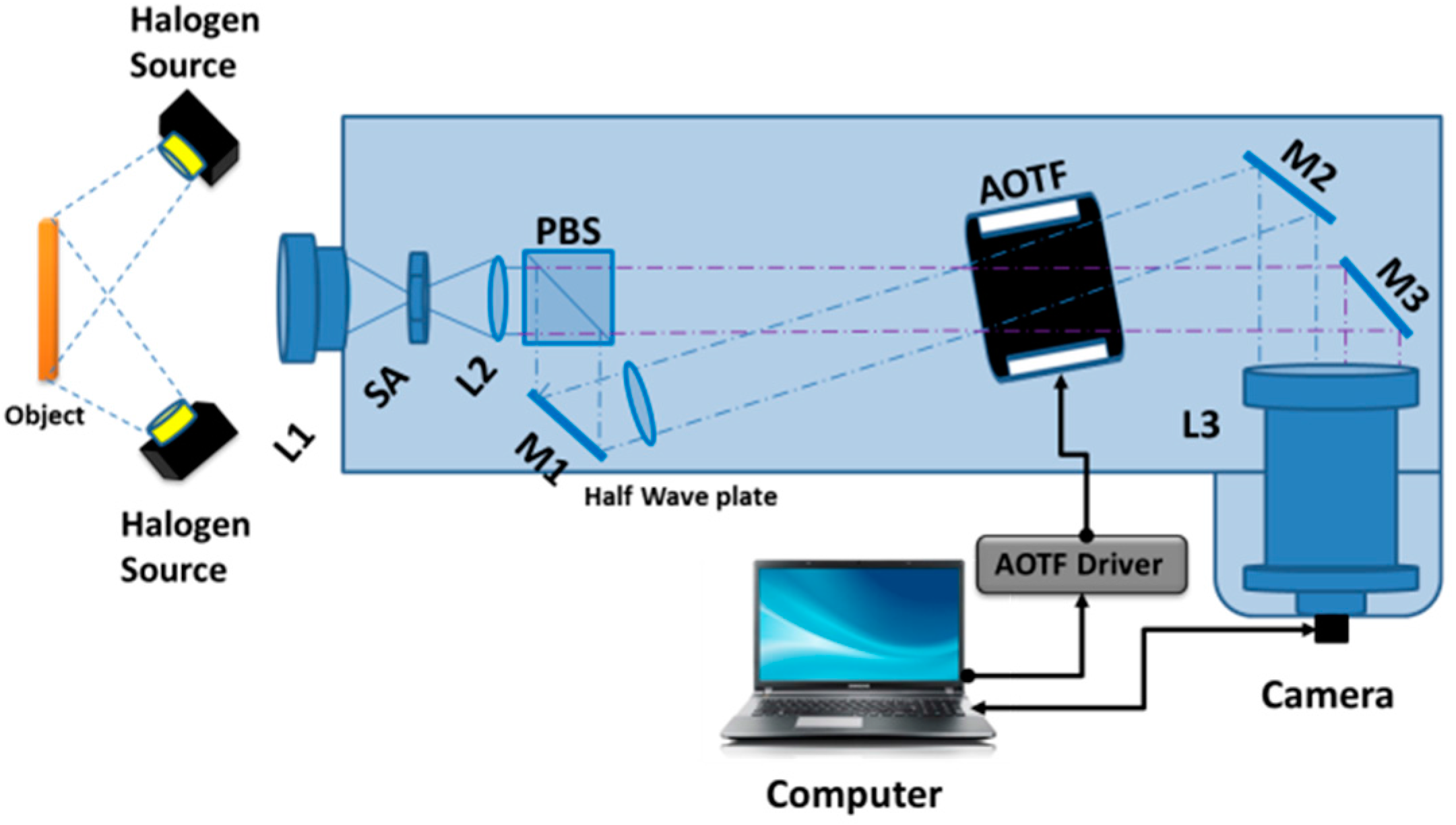
2. Materials and Methods

Compared to the spectroscopy system [22,28], the size of the beam is much larger in an imaging system. Therefore, it is not practical to directly use the two first-order diffracted signals at orthogonal polarization states. Instead, the randomly polarized input signal is separated into two linearly polarized components by a polarizing beam splitter (PBS). Then, one polarization path is rotated 90 degrees by a half waveplate such that both beam paths have the same polarization direction. As shown in Figure 1, two 150-watt tungsten-halogen lamps are used as illumination. Randomly polarized signal from the object is collected by a zoom lens L1 (Canon EF-S 55–250 mm f/4–5.6 IS) and focused at the first focal plane where a square aperture (8 × 8 mm) is used to block background noise. The formed image is then collimated by an achromatic lens L2 (EFL = 250 mm, Thorlabs, Newton, NJ, USA). A polarizing beam splitter (PBS513, Thorlabs) splits the randomly polarized light into two paths with orthogonal polarization states: e and o polarized light. The transmitted o polarization light—which matches the AOTF optimized polarization direction—will continue to incident on an AOTF crystal (TF625-350-2-11-BR1A, Gooch & Housego, Cleveland, OH, USA).
The orthogonally polarized e light is reflected by a mirror M1 to a half-wave (λ/2) plate (Dayoptics, ϕ 25.4 mm, Fuzhou, China). The plate rotates the reflected light polarization by 90°, thereby matching the AOTF crystal input. In order to fit the two rays into the AOTF crystal angular aperture (±2°), the crystal was tilted relative to the system’s optical axis. The rays’ path lengths are designed to be equal (<1 mm) in order to maintain the same magnification and propagation time for potential time-domain applications.
The AOTF now has two input polarized beams fitted within the acceptance angle of the crystal. As such, the AOTF diffracts both beams with the same wavelength and linewidth to different directions. Two mirrors M2 and M3 are positioned to avoid the undiffracted beams while deflecting the two first-order diffracted beams toward the second relay lens L3 (EFL = 250 mm, Thorlabs), which focus the collimated beams onto a CMOS readout camera (2048 × 2048, 5.5 µm pixel size, MQ042RG-CM, Xemia, Munster, Germany). The optical relay lenses L2 and L3 are selected to be replicas in order to convey the object’s image formed at the square aperture with no magnification to the sensor.
The spectral dispersion in the developed imager is accomplished using a large aperture AOTF (11 mm × 12 mm) optimized for imaging applications between 450 and 800 nm. To tune the AOTF to different wavelengths, its driving frequency is switched between 65 and 135 MHz, covering the entire spectral range. A laptop computer workstation is used to control the data acquisition and provides a user interface with a custom developed software program.

3. Experimental Work and Results

The performance of the AOTF-HSI instrument was characterized. First, its throughput was measured and compared to a single polarization AOTF setup and an LCTF system. The system’s spectral resolution and spectral response were then characterized. Imaging spatial resolution, field of view (FOV), and depth of focus (DOF) were also measured.

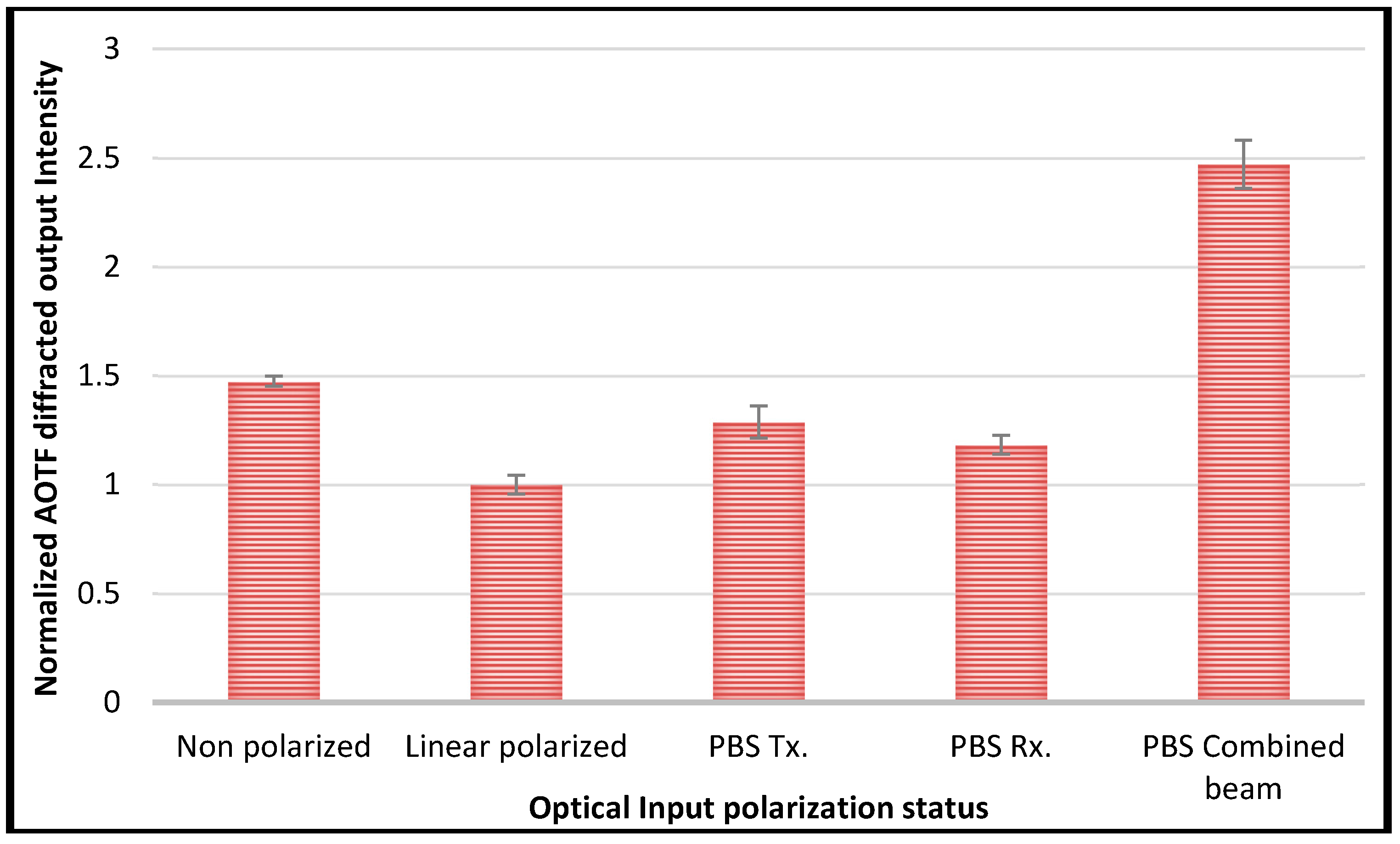
3.1. Optical Throughput Characterization

The throughput of the HSI system is defined as the percentages of the output light at the desired wavelength of the input light. The main benefit of using the dual-input AOTF setup is the improvement in the throughput of randomly polarized signal. To characterize the throughput improvement, a collimated and randomly polarized diode laser light at 650 nm was used as the input. The input and output intensities were measured by an optical power meter (1830C, Newport, Irvine, CA, USA). The throughput was measured in the following three configurations simulating two (#1 and #2) typical conventional AOTF operating modes (i.e., single polarization) and the dual polarization design (#3).
  • Randomly polarized input beam with a single polarization AOTF setup (i.e., laser output directly used as an input passing the AOTF crystal);
  • Single polarization AOTF setup with linearly polarized light input aligned to the optimized polarization direction of the AOTF (laser output going through a linear polarizer);
  • Randomly polarized input beam going through the dual beam setup (i.e., Figure 1).
In the case of #3, in addition to the combined beam throughput, the two polarization beams were measured separately by blocking the one of the polarization path. The results of the measurements are shown in Figure 2.

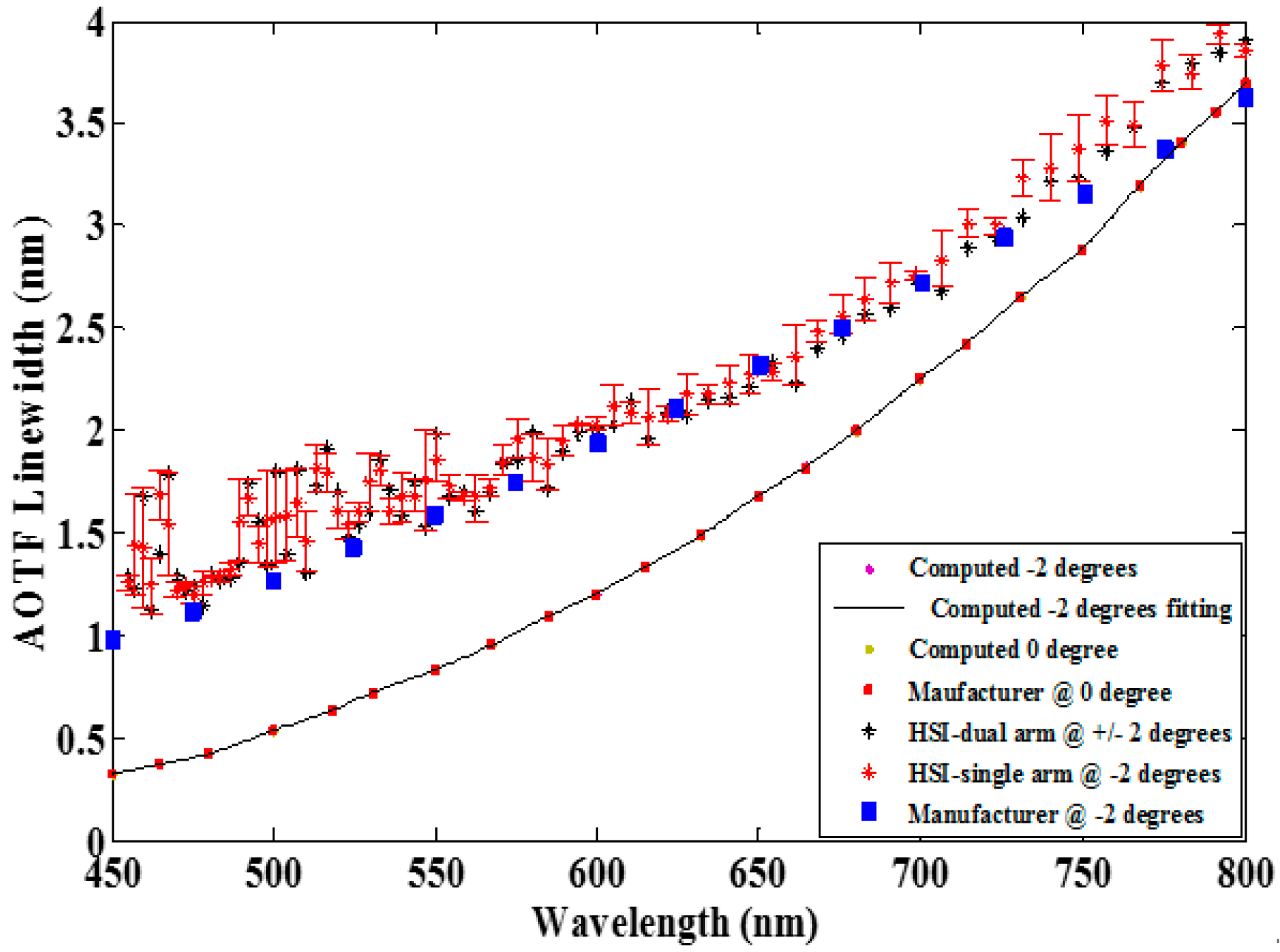
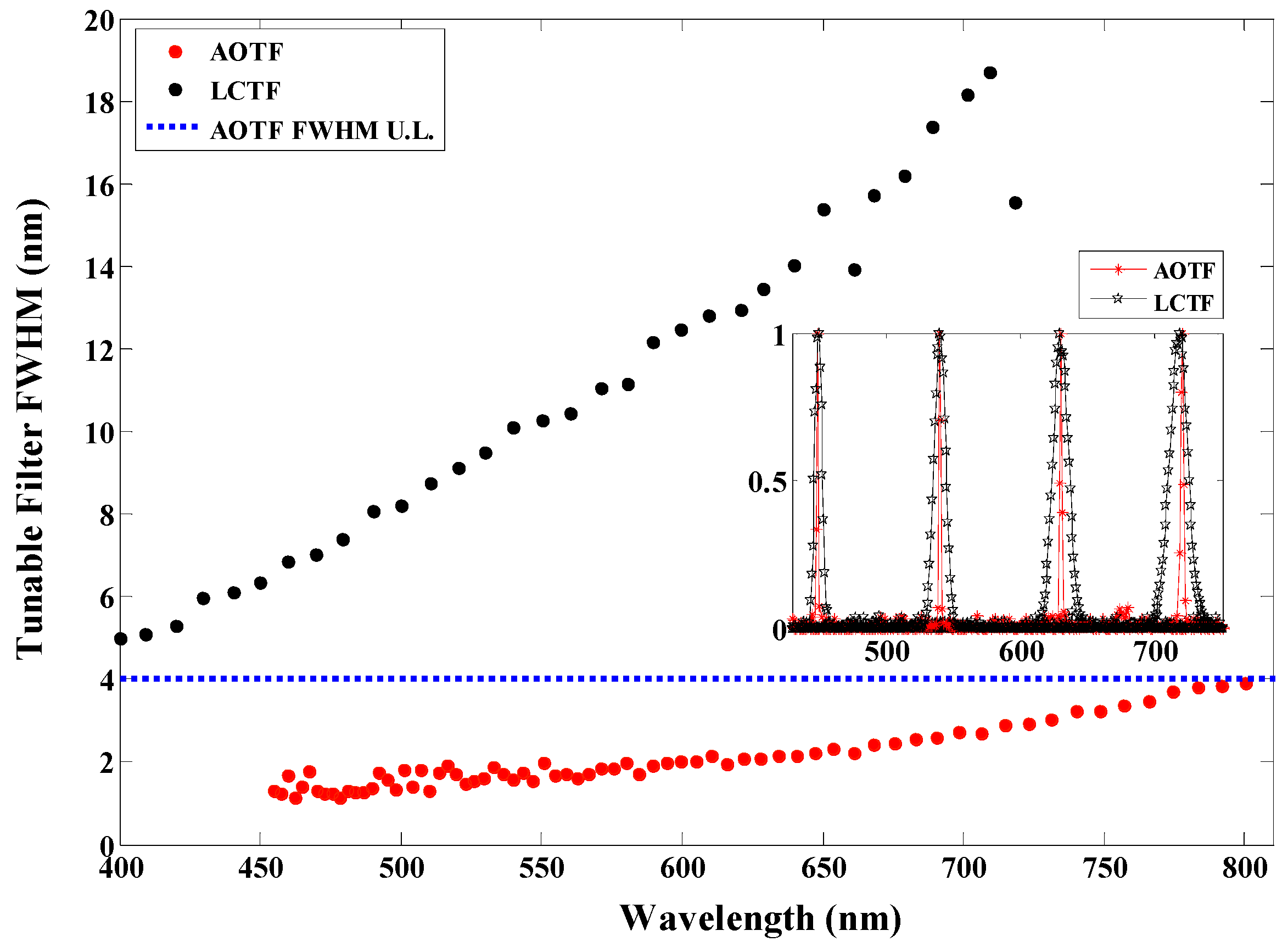
3.2. Spectral Characterization

Each optical component affects the system’s spectral response. The mirrors, lenses, the half-wave ½ λ plate, and the polarizing beam splitter (PBS) were selected to optimize the integrated system performance. A calibrated spectrophotometer (OSM-400, Newport) was used to measure the output with a broadband halogen light source (A20500 Fostec, ACE light source with EKE lamp, Mainz, Germany) as the input.
The AOTF-HSI spectral line-width (FWHM—full width half maximum) was measured across its operating spectral range, as shown in Figure 3. In addition, theoretical values at different incident angles (θi = 0, ±2, ±4 degrees) were computed based on Equation (1)) and plotted for comparison purposes.
  λ = 1.8 π λ 2 / b L   s i n 2 θ i
As shown in Equation (1), the line width ( F W H M =   λ ) of the diffracted band exiting of the AOTF crystal is proportional to the square of the central wavelength ( λ 2 ) when other parameters (the incidence angle ( θ i ), the length of photoacoustic interaction ( L ), and the spectral dispersive constant (b) of the TeO2 crystal) are constants. As a result, the spectral resolution of the AOTF spectrometers reduces (i.e., line width increases quadratically as a function of wavelength). Due to the differences of incident angle, the line width of the dual channel AOTF-HSI configuration is higher than a single beam configuration. As shown in Figure 3, this difference is relatively small when the incident angle is within ±2 degrees.
Figure 3 also shows that the maximum difference between the two channels turned out to be ±0.8 nm at 450 nm and gradually reduced to ±0.1 nm at 800 nm, which is acceptable compared to its spectral resolution and most intended applications.

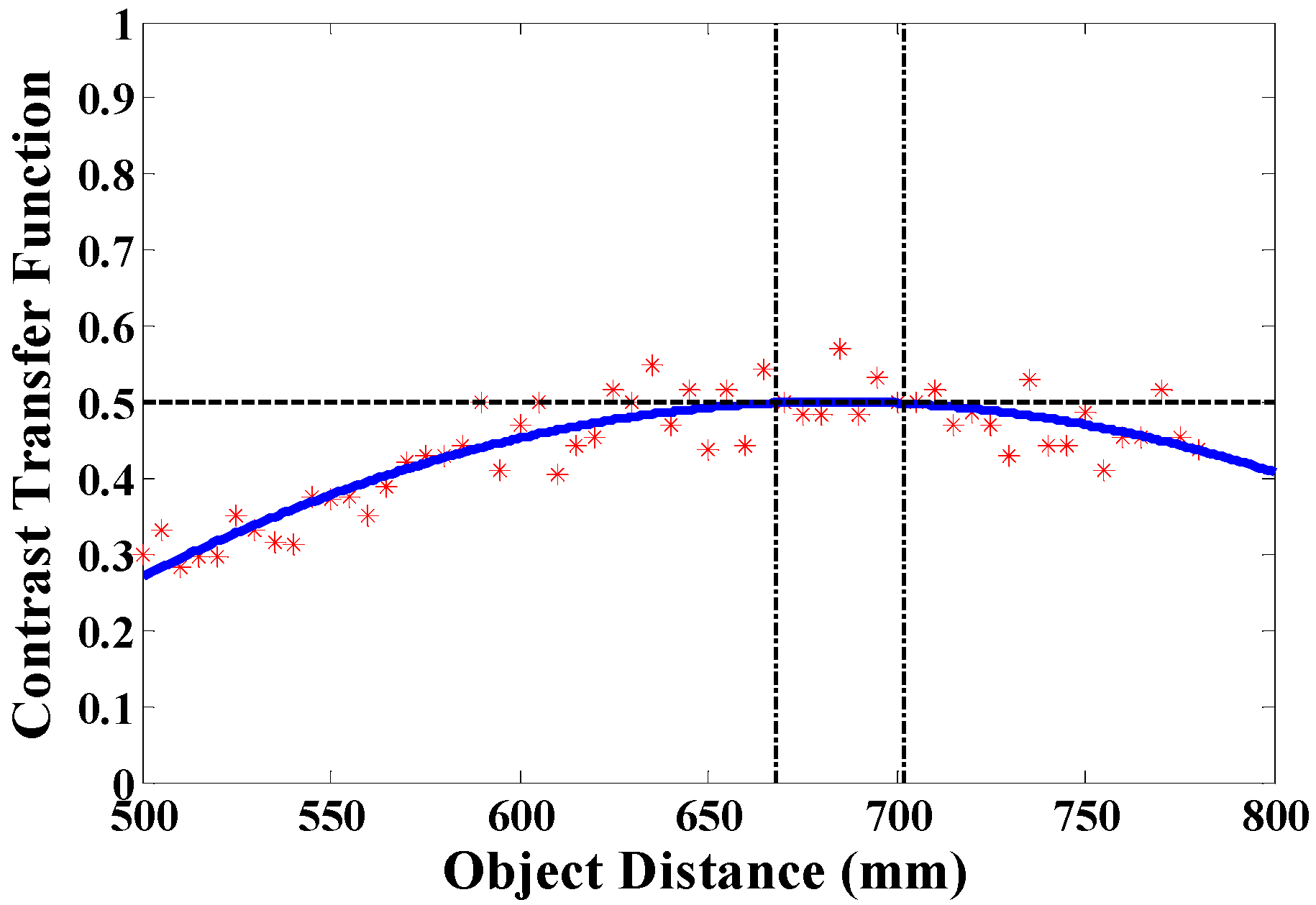
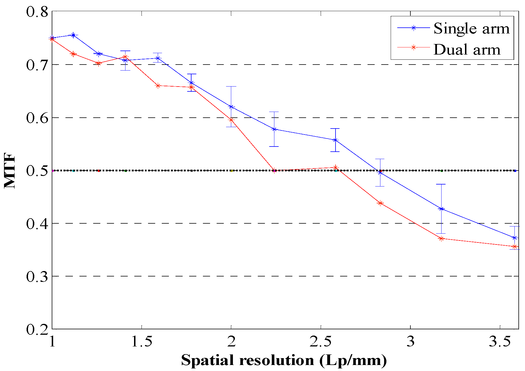
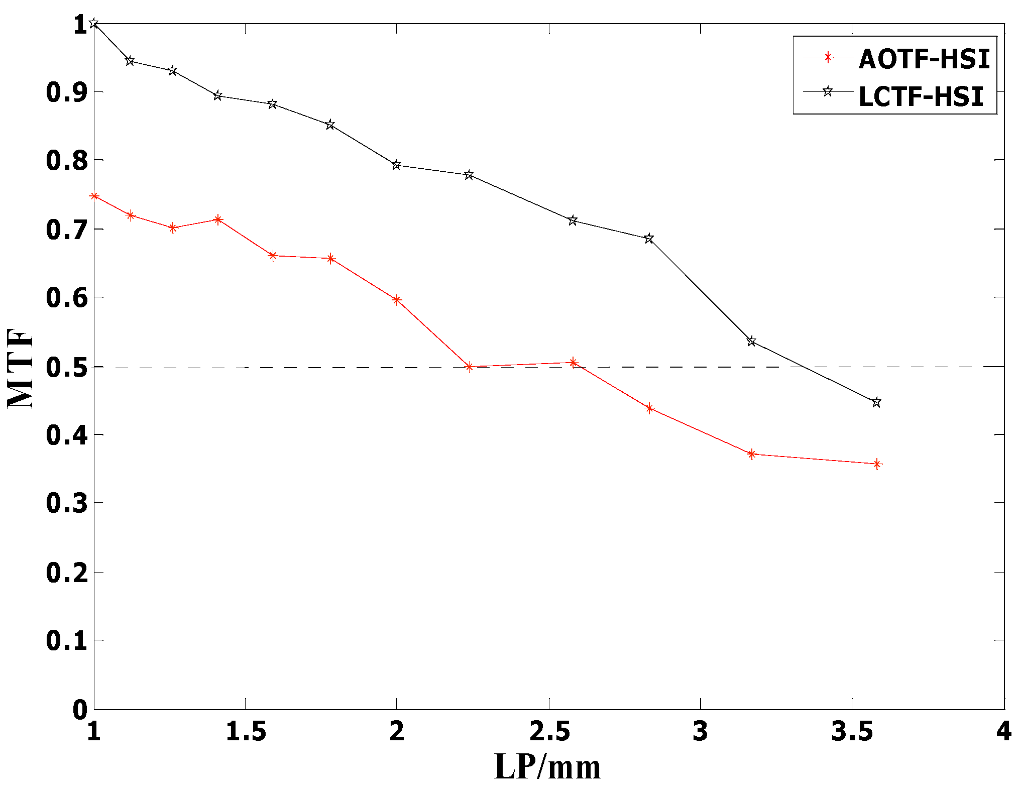
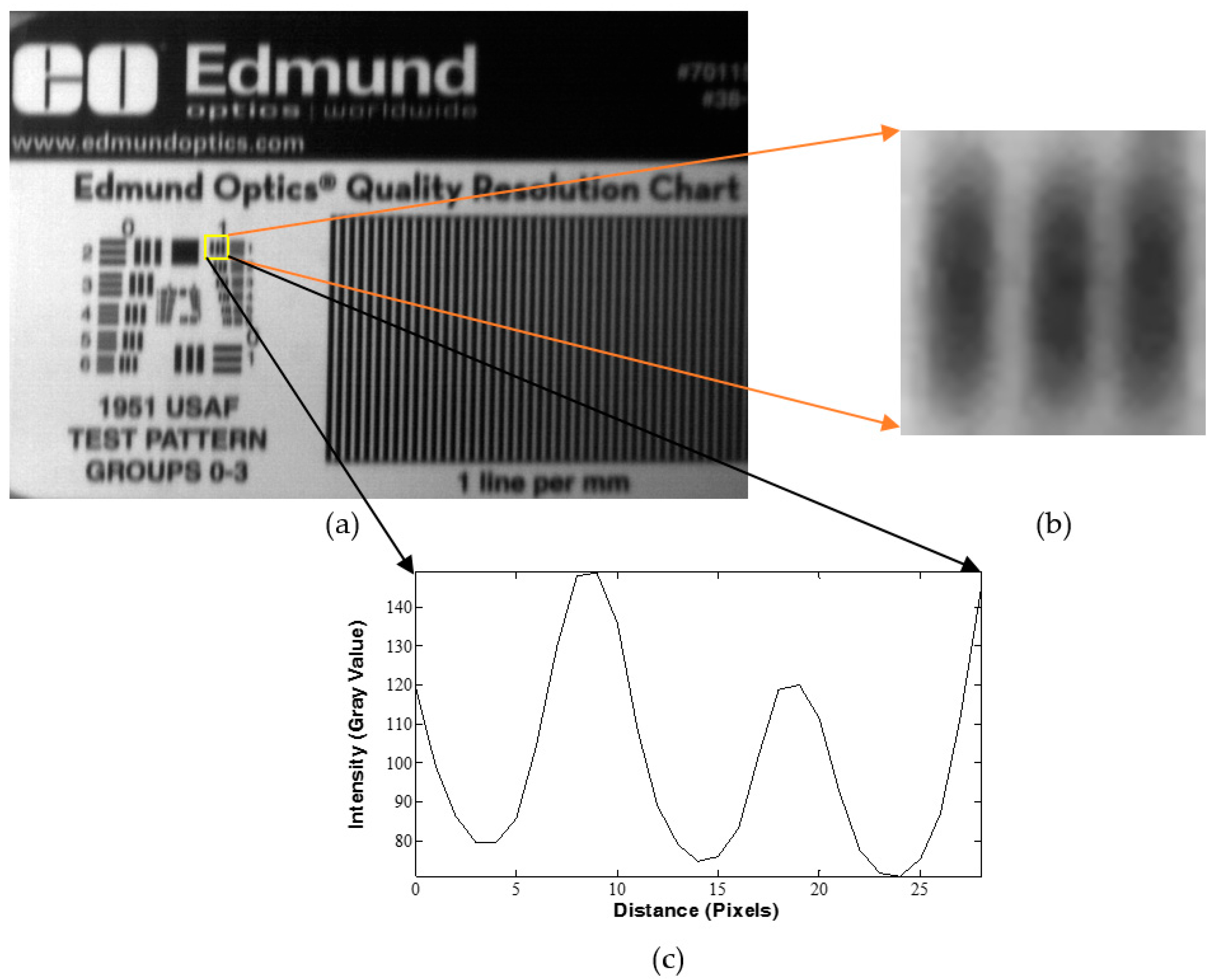
3.3. Spatial Characterization

For imaging application, spatial resolution and depth of field (DOF) are important parameters. To characterize these spatial parameters, a USAF resolution target (USAF-1951, 38-710, Edmund Optics, Barrington, NJ, USA) was used. First, the optimal focal location was determined by scanning the optical axis and the location was determined with the maximum contrast transfer function (CTF), which is defined in Equation (2).
C T F = M a x I M i n I M a x I + M i n I
where M a x I     , M i n I are the maximum and minimum pixel intensities along a line orthogonally drawn across a certain group; an example of the image and intensity changes in the rectangular region is shown in Figure 4.
Figure 5 shows the CTF values of an element (group 1/element-1 = 2 LP/mm, on the USAF-1951 target) before and after the focal spot along the optical axis of the AOTF system. The optimal range was determined to be between 668 mm and 702 mm (CTF ≥ 0.5), which corresponds to the effective DOF of 34 mm [29].
The modulation transfer function (MTF) measurement is commonly computed to characterize the spatial resolution of an optical system. To compute an imaging system’s MTF, the ratio of the acquired image modulation and the original object modulation is accounted as demonstrated in Equation (3) [30]:
M T F = M o d i m a g e M o d o b j e c t
The term Modimage is the measured CTF of the target image captured by the AOTF-HSI, and Modobject is the CTF provided by the USAF target manufacturer. Using a standard test object in Equation (3) implies a unity modulation (i.e., Modobject = 1). As such, the system MTF is directly considered as the modulation of the object captured image. This test characterizes the system’s ability to resolve spatial features. Figure 6 illustrates the AOTF-HSI imaging system’s MTF at an object distance equal to 685 mm.

3.4. Performance Comparison to LCTF

AOTF and LCTF are two typical tunable filter technologies commonly used in hyperspectral imaging. Both have been studied previously for a number of applications, including fluorescence and Raman microscopy [31], as well as laser-induced breakdown spectroscopy [32]. In this study, we report the comparison between both filters for hyperspectral imaging in (1) spectral resolution; (2) spectral selectivity; (3) reliability and image quality; and (4) spatial resolution [33].
An LCTF (400–720 nm, VIS-10-20, Cambridge Research & instrumentation, Hopkinton, MA, USA) was used to replace the AOTF in a setup similar to that shown in Figure 1. Since the LCTF does not require separation of the non-diffracted order light, the alignment is simple and the setup is compact. A wavelength calibration target (erbium oxide; WCS-EO-010, Labsphere, NH, USA) and white standard reflectance target (SRS-99, Labsphere, NH, USA) were used for spectral imaging quality and reliability assessment. A tungsten-halogen light source and two laser lines—He-Ne laser emitting at λ = 633 nm and a diode laser emitting at λ = 675 nm—were used in the characterization experiments.
The spectral and spatial resolution experiments similar to those used in the AOTF experiments were repeated when the LCTF was placed orthogonal to the input beam. This result of the spectral resolution evaluation (shown in Figure 7) demonstrate that the AOTF has significantly better spectral resolution than LCTF.
In order to evaluate AOTF and LCTF in the spatial domain, a USAF-1951 target was used [34]. The modulation transfer function (MTF) for elements of both group zero and one was calculated according to Equation (3), and was plotted as shown in Figure 8.

4. Discussion and Conclusions

We report the development of a dual-polarization path high throughput AOTF-based hyperspectral imaging system. The system operates in the range of 450–800 nm with spectral resolution varying from ~1.5 to 4.1 nm, as a function of the wavelength. The dual path configuration has an increased overall throughput because it makes use of two components of the randomly polarized input light rather than one in the existing single-beam configurations. The dual path AOTF-HSI configuration improves the throughput by 68% compared to the conventional single polarization design in the case of randomly polarized signal.
The performance of the dual-path AOTF-HSI system is characterized and compared to both single path AOTF imager designs and LCTF based HSI system. In addition to the throughput improvement, the AOTF’s spectral linewidth is significantly lower than the LCTF over the entire operating range, since the AOTF has a linewidth of 1.5–4.1 nm while the LCTF linewidth is ~5–19 nm.
In spite of the advantages in the spectral domain, LCTF performs well in the spatial domain. For example, the imaging quality is an advantage for LCTF relative to AOTF, as demonstrated in the MTF plots in Figure 8. The poorer spatial resolution in the dual path AOTF design is attributed to: (1) the combination of the two spatial images when both optical paths onto the detector are not perpendicular; and (2) the two images may not be identical in size and shape due to aberration through different optical paths.
A general strength of AOTF is the high-speed switching between spectral bands within a few µs, while LCTF switches in the ms regime. For time-sensitive applications requiring a high number of spatial channels, AOTF is generally preferred. In addition, AOTF has a broader spectral operating range relative to LCTF.

Acknowledgments

The authors acknowledge that the project is supported in part by the Natural Science and Engineering Council (NSERC) of Canada, Canadian Foundation of Innovation, and the Ontario Research Fund. QF held the Canada Research Chair in Biophotonics. RA is supported by a scholarship provided by the Egyptian Government.

Author Contributions

Q.F., P.S., J.O. and R.B. conceived and designed the experiments; R.A. and J.O. performed the experiments; R.A. and Q.F. analyzed the data; Q.F. and R.A. wrote the paper.

Conflicts of Interest

The authors declare no conflict of interest.

References

  1. Goetz, A.F.H. Three decades of hyperspectral remote sensing of the Earth: A personal view. Remote Sens. Environ. 2009, 113, S5–S16. [Google Scholar] [CrossRef]
  2. Tong, Q.; Zhang, B.; Zheng, L. Hyperspectral remote sensing technology and applications in china. In Proceedings of the 2nd CHRIS/Proba Work. ESA/ESRIN, Frascati, Italy, 28–30 April 2004; pp. 1–10. [Google Scholar]
  3. Gat, N. Imaging Spectroscopy Using Tunable Filters: A Review. In Proceedings of the SPIE, Orlando, FL, USA, 5 April 2000; Volume 4056, pp. 50–64. [Google Scholar]
  4. Gowen, A.; Odonnell, C.; Cullen, P.; Downey, G.; Frias, J. Hyperspectral imaging—An emerging process analytical tool for food quality and safety control. Trends Food Sci. Technol. 2007, 18, 590–598. [Google Scholar] [CrossRef]
  5. Huang, H.; Liu, L.; Ngadi, M.O. Recent developments in hyperspectral imaging for assessment of food quality and safety. Sensors 2014, 14, 7248–7276. [Google Scholar] [CrossRef] [PubMed]
  6. Liang, H. Advances in multispectral and hyperspectral imaging for archaeology and art conservation. Appl. Phys. A 2011, 106, 309–323. [Google Scholar] [CrossRef]
  7. Edelman, G.J.; Gaston, E.; van Leeuwen, T.G.; Cullen, P.J.; Aalders, M.C.G. Hyperspectral imaging for non-contact analysis of forensic traces. Forensic Sci. Int. 2012, 223, 1–3. [Google Scholar] [CrossRef] [PubMed]
  8. Zalevsky, Z.; Ilovitsh, A.; Beiderman, Y. Usage of cornea and sclera back reflected images captured in security cameras for forensic and card games applications. In Optics and Photonics for Counterterrorism, Crime Fighting and Defence IX; and Optical Materials and Biomaterials in Security and Defence Systems Technology, Proceedings of the SPIE, Dresden, Germany, 31 October 2013; SPIE: Bellingham, WA, USA, 2013; Volume 8901, p. 89010I. [Google Scholar]
  9. Yuen, P.W.; Richardson, M. An introduction to hyperspectral imaging and its application for security, surveillance and target acquisition. Imaging Sci. J. 2010, 58, 241–253. [Google Scholar] [CrossRef]
  10. Chao, T.-H.; Cheng, L.-J.; Yu, J.; Reyes, G. Acousto-Optic Tunable Filter Imaging Spectrometers. In Proceedings of the 11th Annual International Geoscience and Remote Sensing Symposium, Espoo, Finland, 3–6 June 1991; Volume 1, pp. 585–588. [Google Scholar]
  11. Glenar, D.A.; Hillman, J.J.; Saif, B.; Bergstralh, J. Acousto-optic imaging spectropolarimetry for remote sensing. Appl. Opt. 1994, 33, 7412–7424. [Google Scholar] [CrossRef] [PubMed]
  12. Huang, F.; Yan, L. Hull vector-based incremental learning of hyperspectral remote sensing images. J. Appl. Remote Sens. 2015, 9, 96022. [Google Scholar]
  13. Lu, G.; Fei, B. Medical hyperspectral imaging: A review. J. Biomed. Opt. 2014, 19, 10901. [Google Scholar] [CrossRef] [PubMed]
  14. Mordant, D.J.; Al-Abboud, I.; Muyo, G.; Gorman, A.; Sallam, A.; Ritchie, P.; Harvey, A.R.; McNaught, A.I. Spectral imaging of the retina. Eye 2011, 25, 309–320. [Google Scholar] [CrossRef] [PubMed]
  15. Kiyotoki, S.; Nishikawa, J.; Okamoto, T.; Hamabe, K.; Saito, M.; Goto, A.; Fujita, Y.; Hamamoto, Y.; Takeuchi, Y.; Satori, S.; et al. New method for detection of gastric cancer by hyperspectral imaging: A pilot study. J. Biomed. Opt. 2013, 18, 26010. [Google Scholar] [CrossRef] [PubMed]
  16. Liu, Z.; Wang, H.; Li, Q. Tongue tumor detection in medical hyperspectral images. Sensors 2012, 12, 162–174. [Google Scholar] [CrossRef] [PubMed]
  17. Panasyuk, S.V.; Yang, S.; Faller, D.V.; Ngo, D.; Lew, R.A.; Freeman, J.E.; Rogers, A.E. Medical hyperspectral imaging to facilitate residual tumor identification during surgery. Cancer Biol. Ther. 2007, 6, 439–446. [Google Scholar] [CrossRef] [PubMed]
  18. De Beule, P.A.; Dunsby, C.; Galletly, N.P.; Stamp, G.W.; Chu, A.C.; Anand, U.; Anand, P.; Benham, C.D.; Naylor, A.; French, P.M. A hyperspectral fluorescence lifetime probe for skin cancer diagnosis. Rev. Sci. Instrum. 2007, 78, 123101. [Google Scholar] [CrossRef] [PubMed]
  19. Cao, Q.; Zhegalova, N.G.; Wang, S.T.; Akers, W.J.; Berezin, M.Y. Multispectral imaging in the extended near-infrared window based on endogenous chromophores. J. Biomed. Opt. 2013, 18, 101318. [Google Scholar] [CrossRef] [PubMed]
  20. Ballabriga, R.; Campbell, M.; Heijne, E.H.M.; Llopart, X.; Tlustos, L. The Medipix3 Prototype, a Pixel Readout Chip Working in Single Photon Counting Mode with Improved Spectrometric Performance. IEEE Trans. Nucl. Sci. 2007, 54, 1824–1829. [Google Scholar] [CrossRef]
  21. Hussain, M.; Chen, D.; Cheng, A.; Wei, H.; Stanley, D. Change detection from remotely sensed images: From pixel-based to object-based approaches. ISPRS J. Photogramm. Remote Sens. 2013, 80, 91–106. [Google Scholar] [CrossRef]
  22. Nie, Z.; An, R.; Hayward, J.E.; Farrell, T.J.; Fang, Q. Hyperspectral fluorescence lifetime imaging for optical biopsy. J. Biomed. Opt. 2013, 18, 096001. [Google Scholar] [CrossRef] [PubMed]
  23. Zhang, C.; Wang, H. The narrow band AOTF based hyperspectral microscopic imaging on the rat skin stratum configuration. J. Eur. Opt. Soc. 2014, 9, 14034. [Google Scholar] [CrossRef]
  24. Li, Q.; Peng, H.; Wang, J.; Wang, Y.; Guo, F. Coexpression of CdSe and CdSe/CdS quantum dots in live cells using molecular hyperspectral imaging technology. J. Biomed. Opt. 2015, 20, 110504. [Google Scholar] [CrossRef] [PubMed]
  25. Gao, L.; Kester, R.T.; Tkaczyk, T.S. Compact Image Slicing Spectrometer (ISS) for hyperspectral fluorescence microscopy. Opt. Express 2009, 17, 313–320. [Google Scholar] [CrossRef]
  26. Jolivot, R.; Vabres, P.; Marzani, F. Reconstruction of hyperspectral cutaneous data from an artificial neural network-based multispectral imaging system. Comput. Med. Imaging Graph. 2011, 35, 85–88. [Google Scholar] [CrossRef] [PubMed]
  27. Hagen, N.; Kudenov, M.W. Review of snapshot spectral imaging technologies. Opt. Eng. 2013, 52, 90901. [Google Scholar] [CrossRef]
  28. Yuan, Y.; Hwang, J.-Y.; Krishnanmoorthy, M.; Ning, J.; Zhang, Y.; Ye, K.; Wang, R.-C.; Deen, M.J.; Fang, Q. High throughput AOTF-Based Time-resolved fluorescence spectrometer for optical biopsy. Opt. Lett. 2009, 34, 1132–1134. [Google Scholar] [CrossRef] [PubMed]
  29. Nouri, D.; Lucas, Y.; Treuillet, S. Calibration and test of a hyperspectral imaging prototype for intra-operative surgical assistance. In Proceedings of the SPIE, Medical Imaging 2013: Digital Pathology, Orlando, FL, USA, 9 February 2013; Volume 11, p. 86760P. [Google Scholar]
  30. Zhang, X.; Kashti, T.; Kella, D.; Frank, T.; Shaked, D.; Ulichney, R.; Fischer, M.; Allebach, J.P. Measuring the modulation transfer function of image capture devices: What do the numbers really mean? In Proceedings of the SPIE, Image Quality and System Performance IX, Burlingame, CA, USA, 25 January 2012; Volume 8293, p. 829307. [Google Scholar]
  31. Morris, H.R.; Hoyt, C.C. Imaging Spectrometers for Fluorescence and Raman Microscopy: Acousto-Optics and Liquid Crystal Tunable Filters. Appl. Spectrosc. 1994, 48, 847. [Google Scholar] [CrossRef]
  32. Stratis, D.N.; Eland, K.L.; Carter, J.C.; Angel, S.M.; Tomlinson, S.J. Comparison of Acousto-optic and Liquid Crystal Tunable Filters for Laser-Induced Breakdown Spectroscopy. Appl. Spectrosc. 2001, 55, 999–1004. [Google Scholar] [CrossRef]
  33. Zhou, P.; Zhao, H.; Zhang, Y.; Li, C. Accurate optical design of an acousto-optic tunable filter imaging spectrometer. In Proceedings of the 2012 IEEE International Conference on Imaging Systems and Techniques (IST), Manchester, UK, 16–17 July 2012; pp. 249–253. [Google Scholar]
  34. Sengul, O.; Turkmenoglu, M.; Yalciner, L.B. MTF Measurements for the Imaging System Quality Analysis. Gazi Univ. J. Sci. 2012, 25, 19–28. [Google Scholar]
Figure 1. Schematic of the dual polarization acousto-optic tunable filter (AOTF)-based hyperspectral imaging (HSI) system. L1: zoom lens; SA: square aperture acting as field aperture; L2, L3: achromatic lenses; M1, M2, M3: flat mirrors; PBS: polarizing beam splitter. The optical imaging system is enclosed in an enclosure (shaded area) to ensure portability.
Photonics 05 00003 g001
Figure 2. The diffracted light intensity of the AOTF crystal in: (1) randomly polarized input directly passing an AOTF; (2) linearly polarized input (i.e., #1 + linear polarizer) and directly passing an AOTF (polarization aligned with the AOTF optimal direction); and (3) randomly polarized input (i.e., #1) going through the dual polarization setup. The two polarizations paths were measured separately (PBS transmitted, PBS reflected) in addition to the combined beam (PBS dual beams), respectively. All the displayed diffracted intensities are normalized with respect to the linear polarized input.
Photonics 05 00003 g002
Figure 3. The AOTF-HSI imaging spectrometer line-width (FWHM—full width half maximum) for both single arm and dual arms, compared with the manufacturer line-width data in addition to a theoretical computational data for different optical input incident at angles (0, ±2 degrees). The standard deviation is computed for each arm in the developed AOTF-HSI system and plotted as error bars for the single arm curve.
Photonics 05 00003 g003
Figure 4. (a) A resolution (USAF-1951) target is imaged by the AOTF-HSI system at 700 mm displacement. Group-1/element-1—zoomed in (b)—is enclosed in a yellow dotted rectangle. (c) The intensity was plotted, where maximum and minimum intensities are identified to calculate the contrast transfer function (CTF) at this range.
Photonics 05 00003 g004
Figure 5. Measured contrast transfer function (CTF) values (dot), for the spatial target group-1/element-1, along the optical axis before and after the focal spot. X-axis is the absolute distance between the target and the front of the lens. The dashed line is the quadratically fitted curve, while the vertical dashed lines mark regions with CTF ≥ 0.5.
Photonics 05 00003 g005
Figure 6. The AOTF-HSI imager modulation transfer function (MTF) plot obtained by imaging USAF-1951 spatial target.
Photonics 05 00003 g006
Figure 7. The imager’s spectral resolution evaluation in the case of switching between AOTF (red circles) and liquid crystal tunable filter (LCTF, black circles) along the wavelength operating range for each filter. Samples of filtered/diffracted bands are also included in the embedded figure. A blue dotted horizontal line is drawn with a value equal to the lower spectral resolution limit of the AOTF-HSI. This line illustrates that the AOTF has superior linewidth in contrast with the highest spectral resolution of the corresponding LCTF-HSI.
Photonics 05 00003 g007
Figure 8. Modulation transfer function of both tunable filters, LCTF and AOTF, imaging USAF-1951 reflection pocket target group 0 and 1.
Photonics 05 00003 g008

