Article

Non-Uniform Modal Power Distribution Caused by Disorder in Multimode Fibers

Department of Information Engineering, Electronics and Telecommunications (DIET), Università degli Studi di Roma Sapienza, Via Eudossiana 18, 00184 Rome, Italy
Photonics 2026, 13(2), 129; https://doi.org/10.3390/photonics13020129
Submission received: 30 December 2025 / Revised: 16 January 2026 / Accepted: 27 January 2026 / Published: 30 January 2026
(This article belongs to the Special Issue The Many Paths of Light: Unraveling Multimode Optical Fibers)

Abstract

The evolution of modal crosstalk in multimode fibers is investigated using four different experimental and numerical approaches. Results converge to demonstrate that the fiber disorder alone is capable of generating steady states characterized by non-uniform modal power distributions, which promote the lower-order modes at the expense of the higher-order ones and are properly described by a weighted Bose–Einstein law.

1. Introduction

Multimode fibers (MMF) [1,2] and multicore fibers (MCF) [3,4] support the simultaneous propagation of orthonormal modes characterized by different field distribution F p ( x , y ) , propagation constant β p , and fiber loss α p . In graded-index multimode fibers (GRIN), the fiber index profile is commonly parabolic-shaped [5], and the fiber modes compose groups of quasi-degenerate modes with the same propagation constant β j .
MMFs and MCFs were rediscovered in an attempt to solve the capacity problem in optical networks [6,7] using the space-division multiplexing (SDM) technique [8], which adds a further degree of freedom for increasing the transmission capacity by multiplexing channels into the different orthonormal modes or cores of the fiber.
One of the main transmission impairments of MCF and MMF low-power systems arises from fiber imperfections, consisting of micro and macro bendings, fiber radius, and index random changes, which cause the random-mode coupling effect (RMC) [9,10,11], characterized by a random exchange of power between orthonormal modes of a fiber. A second detrimental effect is the mode-dependent loss (MDL), where different non-degenerate modal groups experience different linear losses [1]. As it will be shown, both effects contribute to generating non-uniform modal power distributions, where the lowest-order modal groups (LOMs) are promoted at the expense of the highest-order ones (HOMs).
In the literature, numerical simulations of multimode fibers that include RMC provided conflicting results, depending on the model used for fiber disorder. For example, in [12,13], disorder was modeled using a random potential δ V ( x , y , z ) = μ ( z ) g ( x , y ) , with μ ( z ) a stochastic function with zero mean and < μ ( z ) μ ( 0 ) > = σ b 2 exp ( z / L c ) , being L c the RMC correlation length and with disorder arising from an elliptical fiber structure of the type g ( x , y ) = cos ( b x x / x 0 ) cos ( b y y / y 0 ) ; this approach provided steady states where the power distribution between modes was nearly uniform.
In [14], a matrix propagation model was used, where the end-to-end fiber transfer matrix was obtained as the product of several sections’ transfer matrices. Different cross-talk patterns were obtained, depending on the model used for the section transfer matrices (homogeneous perturbation drift model, propagation constant drift model).
In this work, we use four different experimental and numerical approaches to study the steady state modal power distribution produced by the RMC in several kilometers of GRIN fiber. Specifically, the four approaches are as follows:
(i) Numerical simulations based on coupled generalized nonlinear Schrödinger equations (GNLSE) [15,16], modified to include the effects of multimode fiber disorder. The model adopted for RMC is the well-known field coupling model [11,17], using modal coupling coefficients depending on fiber index perturbations Δ n ( x , y , z ) with uniform random distribution and on overlapping integrals between the transverse fields F p ( x , y ) of the coupled modes.
(ii) Numerical simulations based on the well-known power-flow equations model (PFE) [9,10,18], describing the bi-directional flow of power between fiber modal groups. Power flows towards LOMs and HOMs are not symmetrical, causing the steady state modal power distribution to be non-uniform.
(iii) Experiments in which low-power, Gbit/s pulses were transmitted over several kilometers of GRIN fiber and input (output) modes were coupled (decomposed) using modal multiplexers based on multi-plane light conversion (MPLC) technology [19]. In the experiments, the Kerr and Raman nonlinearities were negligible, and RMC was not artificially forced but was caused by the natural imperfections of a commercial GRIN fiber.
(iv) Experiments recalling case (iii) with low-power pulses replaced by single-photon pulses and power meters by photon-counting techniques. Those experiments confirmed that a non-uniform output distribution is produced even in the ergodic case of single-photon exchanges between interacting modes.
The four approaches converged, providing similar results, confirming that RMC alone is capable of generating steady states characterized by non-uniform modal distributions in a GRIN fiber; the distributions promote the LOMs at the expense of the HOMs and are properly described by a weighted Bose–Einstein law (wBE) [20,21]. In each of the four approaches, the MDL was characterized and properly isolated to measure the contribution of the individual effects.
The rationale for theoretically, experimentally, and thermodynamically characterizing the steady state power distribution of modes is to simplify the design of multimode fiber SDM systems by using simple equations to predict the effects of crosstalk caused by fiber disorder.

2. Materials and Methods

2.1. Experiments

For the experiment in the classical linear regime, a continuous wave laser at λ = 1550 nm, with a 10 kHz linewidth (Thorlabs TLX1, Bergkirchen, Germany), was carved to a train of pulses at 1 Gb/s by an optical intensity modulator (IM, Exail MX-LN-10, Denver, CO, USA) driven by an FPGA; pulsewidth was 330 ps. The signal was split by a 1 × 16 coupler and applied to different optical delay lines before being coupled to the transmission line (Figure 1).
Signals were applied to the different modal inputs of a modal multiplexer (Cailabs Proteus C-15, Rennes, France) characterized by multi-plane light conversion (MPLC) technology [19]; the multiplexer coupled the power of each input to one of the first 15 Laguerre–Gauss modes ( L G p with p = 1 , 2 , , 15 ) of a GRIN OM4 fiber (Thorlabs GIF50E); the fiber was capable of supporting Q = 10 groups of quasi-degenerate modes at 1550 nm, corresponding to M = 55 modes per polarization (group j includes j quasi-degenerate modes); hence, only the first 5 groups out of 10 were populated at the input. One of the input signals was measured by a power meter.
Two spans of OM4 fiber (20 m or 5 km) were alternatively spliced to the multiplexer/demultiplexer. The parameters of the OM4 fiber at the wavelength λ = 1550 nm are as follows: dispersion β 2 = 28.0 (or −28.6) ps2/km for mode 1 (or mode 15), higher-order dispersion β 3 = 0.15 ps3/km, material loss α = 5.0 × 10 5 m−1, Kerr nonlinear coefficient n 2 = 2.6 × 10 20 m2/W, fiber radius a = 25 μ m.
At the output, a twin modal demultiplexer was used to decompose the received beam into modes. The power content of the first 15 Laguerre–Gauss modes was measured by a power meter.
The modal power at the input of the OM4 was 7.4 μ W, corresponding to a pulse energy and peak power of 7.4 fJ and 21 μ W, respectively. The dispersion length, where dispersion-induced pulse broadening is not negligible, is L D = 1402 km; the nonlinearity length, where the Kerr nonlinearity cannot be neglected, is L N L = 88,700 km; hence, pulses propagated in the linear regime and conserved their shape in the experiment; however, they were subject to material and modal loss, and RMC caused power exchange among degenerate and non-degenerate modes. The pulsed regime was used to reduce the phase coherence between different modes, which could cause fluctuations in the decomposed modal power. With this choice, the modal power fluctuation at the output of the demultiplexer was less than 10%, which represents the accuracy of the experiment.
In the experiment in the quantum regime, pulses were attenuated to one photon per pulse per mode at the input of the OM4; input and output power meters were replaced by single-photon detectors (ID Qube NIR, Genève, Switzerland) in gated mode with 10% efficiency; histograms were counted using a time controller (IDQ ID1000) with 25 ps resolution.

2.2. Numerical Model for GNLSE

The generalized nonlinear Schrödinger equation model (GNLSE) for the multimode fiber is a derivation of [15,16], modified to include the presence of RMC. The complex amplitudes for modes p evolve as
A p z , t z = i β 0 p β 0 A p β 1 p β 1 A p t + i n = 2 4 β n p n ! i t n A p α p λ 2 A p + i n 2 ω 0 c l , m , n Q p l m n { 1 f R A l A m A n * + f R A l h A m A n * } .
The right-hand side terms of Equation (1) describe the following: modal dispersion, four orders of chromatic dispersion, wavelength-dependent losses, and nonlinear Kerr and Raman terms, respectively. The Q p l m n are cross-terms corresponding to the inverse of the effective modal areas, providing appropriate weights to inter-modal four-wave mixing (IM-FWM) and inter-modal stimulated Raman scattering (IM-SRS) terms. The Raman term in Equation (1) contributes with a fraction f R = 0.18 ; the expression h A m A n * denotes time convolution with the Raman response function h ( t ) , with typical time constants of 12.2 and 32 fs [22]. In the simulations presented in this work, Kerr and Raman nonlinearities are included, although they produce no effect.
Disorder-induced RMC is accounted for by a simulation step introduced every L c meters, being L c the RMC correlation length; the applied equation is
A p z , t z = i m p q m p A m z , t .
The coefficients q m p account for linear RMC and are associated with random imperfections of the refractive index profile due to macro- and microbending, core deformation, and random index changes. Here, we suppose that RMC occurs both among quasi-degenerate and non-degenerate modes; they are calculated at each step as [11,17]
q m p = π λ n e f f ( p ) I m I p F m ( x , y ) F p ( x , y ) Δ n 2 ( x , y ) d x d y ;
in Equation (3), F m and F p are the modal transverse field profiles with intensity integrals I m , I p , respectively; n e f f ( p ) is the effective index for mode p, which is responsible for the asymmetry q m p q p m ; the random fluctuation of core index, which models the disorder, is related to a random variable r a n d ( x , y ) uniformly distributed between 0 and 1 as
Δ n ( x , y ) = [ 2 r a n d ( x , y ) 1 ] R M C e x ,
being R M C e x a RMC amplitude for Δ n 2 ( x , y ) .
After Equation (2) is applied during an RMC step, the total power is controlled so that it does not undergo discontinuity with respect to the value before the step.

2.3. Numerical Model for Power Flow Equations

In the linear regime, RMC in multimode fibers is properly modeled by the well-known power-flow diffusive equations (PFE); the model does not account for modal degeneracy and applies to the total power in modal groups j = 1 , 2 , , Q . If P j is the power of the j-th mode group, the power exchange among adjacent non-degenerate modal groups is described by [9,10,18], which brings to the equations [10]
P j ( z + L c ) = D L c Δ m 2 D L c 2 m Δ m P j 1 ( z ) + 1 2 D L c Δ m 2 ( α 0 + A m 2 ) L c P j ( z ) + D L c Δ m 2 + D L c 2 m Δ m P j + 1 ( z ) ,
with m ( j ) = j 1 , D and α 0 (1/m) the coupling coefficient and linear losses, respectively, A the modal loss coefficient, Δ m = 1 the modal step and L c the RMC integration step. In Equation (5), power flows in both directions, from group j down to group j 1 and up to j + 1 ; after consecutive integration steps, a cascading effect is produced, causing the coupling of non-adjacent groups. However, in Equation (5) the coupling coefficients from j down to group j 1 and up to j + 1 are different, promoting j 1 ; this produces asymmetric flows of power which promote the LOMs. In [10], the formation of stationary states with non-uniform modal distributions has already been observed.
Mode coupling among quasi-degenerate modes and polarizations into groups is neglected because it is so fast that statistical modal equipartition into groups can be assumed; it is then meaningful to calculate the mean modal content into groups as | f j | 2 = 2 P j / ( g j P t o t ) , with g j = 2 j the group degeneracy and P t o t the total power in the multimode fiber.
Numerical simulations will be used in the following sections to demonstrate the universality of the effects observed in experiments. In particular, we will show how Bose–Einstein thermodynamics can describe, both in experiments and simulations, the modal distributions generated by RMC and summarize them with simple thermodynamic parameters.

3. Results

3.1. Linear Regime Experiment

As a first test in the linear regime, material loss was measured by coupling power to the fundamental mode L G 1 and measuring the total output power from 20 m and 5 km of fiber. The comparison provided α = 0.19 dB/km. Insertion loss of modal groups was measured by applying power to all quasi-degenerate modes of a group and measuring the total output power using 20 m of fiber; this included the loss from the multiplexer/demultiplexer devices, while the fiber loss was negligible. The resulting transmittances, in linear scale, were I L j = 0.49 , 0.36 , 0.38 , 0.38 , 0.37 for groups j = 1 , 2 , , 5 , respectively.
Mode-dependent loss (MDL) was measured by applying power to and measuring power from all modes of a group, using 5 km of fiber, and normalizing to material loss and insertion loss [21]. The group transmittance related to the modal loss was found to be properly described by M D L j = e x p [ A ( j 1 ) 2 L ] with L = 5000 m and A = 4.4 × 10 6 m−1. This MDL estimate is a worst-case scenario; a small fraction of the power lost by the group due to crosstalk is considered MDL. Normalizing the modal distributions to an MDL estimated in this way yields even more uniform distributions than would be obtained with an exact estimate.
After having characterized the system losses, equal power was applied to the modes of one group j, or to all input modes, and the output power was measured from the individual modes p. Output power P p was measured from the 15 modes, calculating the mean and standard deviations over 60 s acquisitions; the output mean modal power fraction was calculated by dividing the insertion loss I L j and the modal loss M D L j and respecting the condition j = 1 5 j | f j | 2 = 1
| f j | 2 = 1 j I L j M D L j P t o t p = j ( j + 1 ) / 2 j + 1 j ( j + 1 ) / 2 P p .
This was done with the purpose of estimating the power transfer between modal groups caused solely by RMC by normalizing modal and insertion losses. The calculation of the mean modal power fraction is justified by the fact that the modal coupling between modes of the same group and between polarizations, is so fast that statistical equipartition of power between them can be assumed.
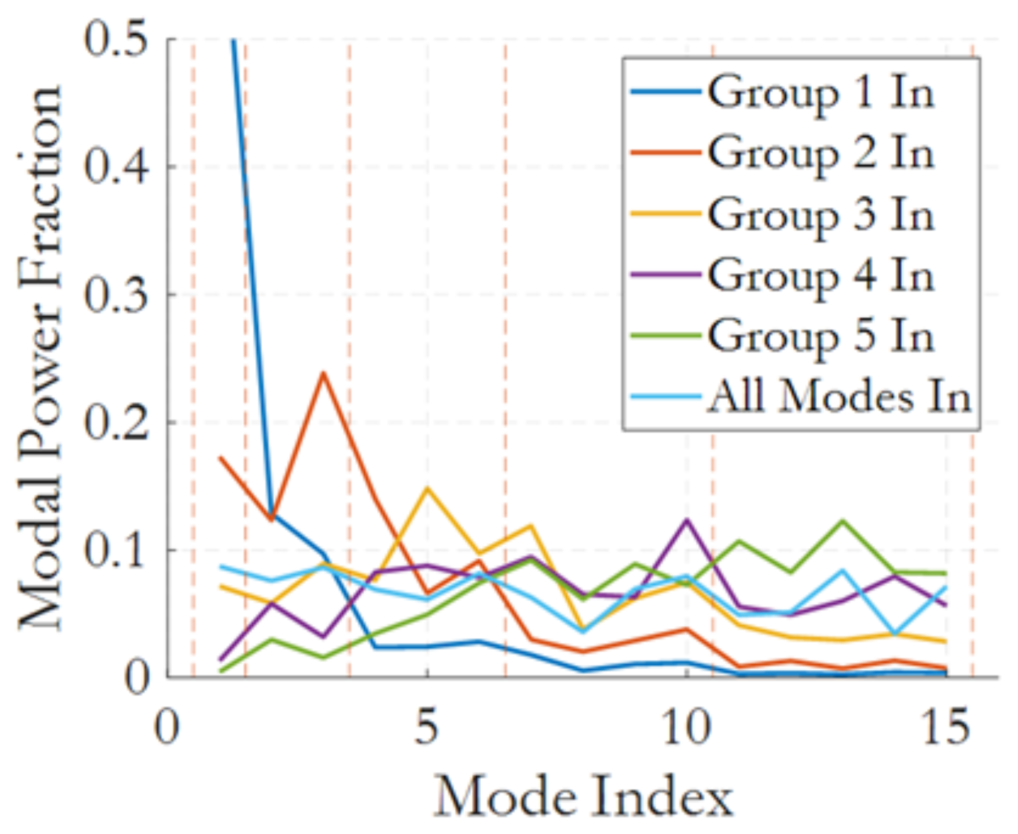
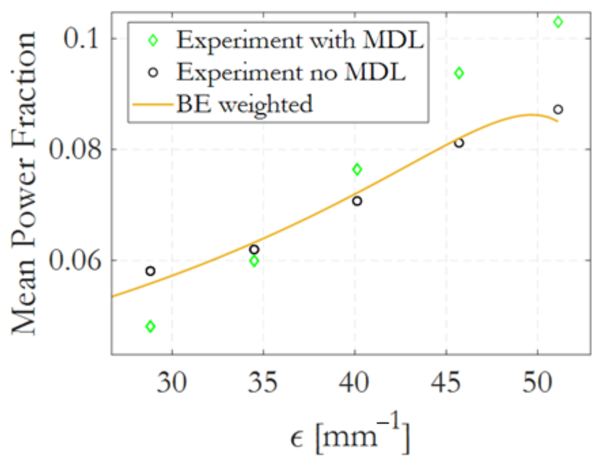
Figure 2 provides the modal fractional power after normalizing to I L j M D L j , when power is applied to the individual modal groups or to all modes. Also, curve ’All Modes In’ in particular shows a non-uniform power distribution at the output; LOMs are promoted by an asymmetric power flow between modal groups, which will be discussed later. This property is more evident in Figure 3, where the average modal power fractions are calculated using Equation (6), when all input modes are uniformly excited. The mean power fraction of modal groups is represented vs. the group eigenvalues, defined as ϵ j = β j β j = Q ; group j = 1 has the larger eigenvalue. In the figure, both output distributions, including and not including MDL, are reported, demonstrating that the preferential power flow toward the fundamental mode is not solely related to modal losses.
The limitations imposed by the MPLC multiplexers in terms of number of modes permit estimating the modal distribution only for the first five modal groups. However, the experimental Figure 2 shows that upon excitation of the LOMs at input, power tends to remain limited to the LOMs and hardly diffuses to the HOMs; for this reason, as a first approximation, we can consider the contribution of the unexcited HOM modes at the input to be negligible at the output.
It was demonstrated in [20,21] that any physical process capable of mixing power among all modes, with negligible variation in the total number of photons N = j n j and internal energy U = j β j n j , being n j the population of a group, produces an output modal distribution described by a weighted Bose–Einstein function (wBE), which corresponds to a maximum Boltzmann entropy of the multimode system. The mean modal power fraction of group j is
| f j | 2 = 2 ( g j 1 ) g j γ 1 exp μ + ϵ j T 1 .
In Equation (7), | f j | 2 = 2 n j / ( γ n 0 g j ) is the mean modal power fraction, over two polarizations, in modal group j. γ is proportional to the input pulse power, μ = μ + β j = Q , with μ (1/m) a chemical potential and T (1/m) an optical temperature. μ and T are two degrees of freedom for fitting Equation (7) to the experimental data. The γ parameter is free at only one intermediate pulse energy; for other energies, it must scale proportionally to the input power or N; the second constraint is the respect of the conservation law j = 1 Q ( g j / 2 ) | f j | 2 = 1 . Temperature T / γ describes how violently the field fluctuates across modes; low values of T / γ denote modal condensation. Chemical potential μ describes how many photons occupy the lowest-energy modes; when approaching thermalization, chemical potential approaches the propagation constant β 1 .
The state equation associated with Equation (7) is S E 1 + S E 2 =0, with
S E 1 = U N = j = 1 Q β j j | f j | 2
S E 2 = μ + ( 2 M Q ) T γ .
After fitting the experimental data using the wBE, the R-squared accuracy parameter of the fit and the error of the thermodynamic state equation, defined as ϵ S E = ( S E 1 + S E 2 ) / ( S E 1 S E 2 ) , are methods to verify the effective thermalization of the output modal distribution. The assumption of negligible variation for U and N, a condition for the validity of Equation (7), is generally verified in experiments where the RMC is responsible for the power exchange between modes. For example, in the case of transmission in an OM4 GRIN fiber, the modes supported at λ = 1550 nm are M = 55 per polarization, for a total of Q = 10 modal groups; the propagation constants of the different groups vary from β 1 = 5.91 × 10 6 m−1 to β 10 = 5.86 × 10 6 m−1. Even in the extreme case in which the RMC causes a total transfer of power from group j = 10 to group j = 1 , the internal energy variation is Δ U / U = ( β 10 β 1 ) / β 10 = 0.0087 . The number of photons N in the case of linear transmission is represented by the average power of the signal or by the energy of the pulses launched into the fiber; the variation of N is negligible as long as the linear losses of the fiber are small, i.e., up to a few kilometers of fiber.
An alternative law, the Rayleigh-Jeans (RJ) [23], is commonly used in the literature when nonlinear optical effects cause the modal power scrambling; we will see that this second law is not able to properly describe the distribution of the LOMs in the linear case, when RMC is responsible for modal power flow.
In Figure 3, it is reported a fit of the output distribution normalized to the MDL, using Equation (7) on the demultiplexed mean power fractions. Correspondence of the experimental distribution to the wBE is good, with parameters T = 4.73 × 10 6 m−1, μ = 6.98 × 10 4 m−1, γ = 3715 , and with a fit R-squared of 0.97; the error of the state equation is ϵ S E = 0.0081 , indicating the achievement of a steady state. Hence, a uniform modal excitation at input has provided a non-uniform modal distribution at the output, even after removing the modal loss. Noise amplification effects when compensating the MDL are negligible, considering the high values of power fraction in the transmitted modal groups.

3.2. Linear Regime Simulation

In order to demonstrate the universality of the steady state distributions observed in the experiment of Figure 3, numerical simulations of linear regime transmission were performed in a multimode OM4 fiber, using the coupled-mode GNLSE model of Equations (1) to (4).
A realistic transmission system was tested, with modal channels composed of trains of 64 encoded pseudo-random pulses at 40 Gb/s per channel, λ = 1550 nm, and femto-Joule pulse energy to prevent the nonlinear effects. Q = 10 modal groups and M = 55 modes were coupled at the input with the same power; hence, 55 coupled Equations (1) were used. Transmission distance was L = 1 km and RMC correlation length L c = 2 m; the RMC randomly scrambled the modal power 500 times over the transmission line; a large R M C e x t = 10 5 was set to observe a considerable power flow. The modal distribution was recorded after each RMC step, repeating the runs 10 times. To reduce statistical fluctuations, the distributions were averaged over 10 runs, and a moving average over 25 consecutive L c steps (50 m) was then applied.
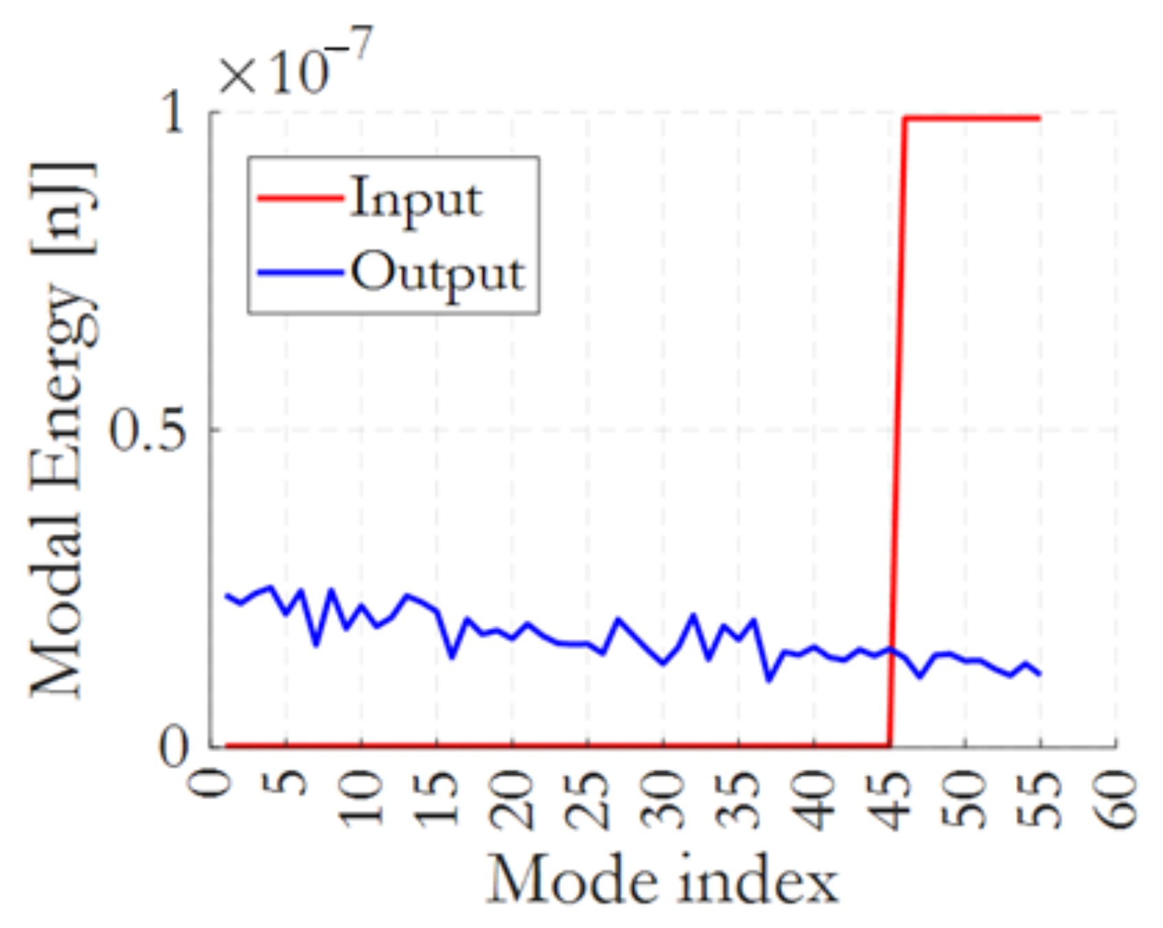
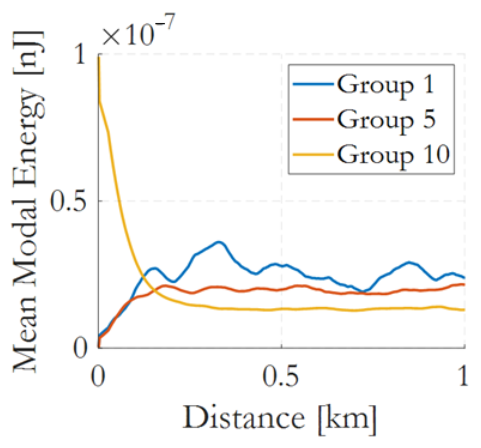
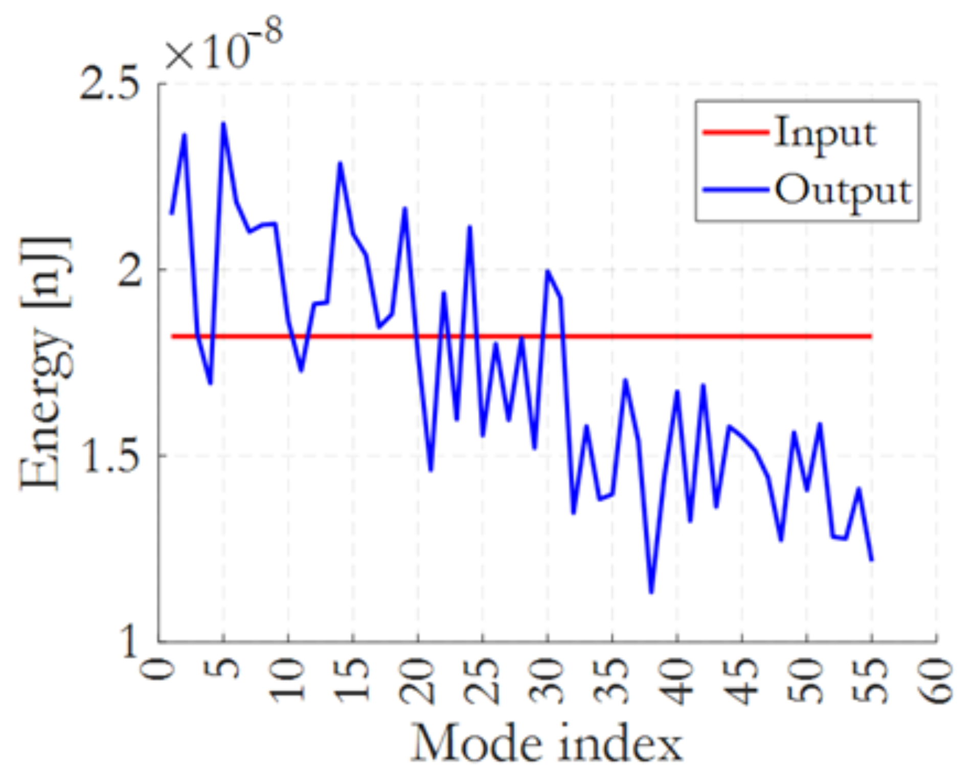
As a first simulation, equal input power was applied only to modes 46 to 55 (modal group 10), leaving the other groups unpopulated. Figure 4 shows the modal energy distribution at the input and output (energy is calculated over the simulation window propagating 32 pulses and 32 spaces per mode); power appears to reorganize to a non-uniform output distribution, which promotes the LOMs. The mean energy of the modal groups 1, 5, and 10 is represented in Figure 5 vs. distance; group 1 (10) experiences the larger modal energy increase (reduction), demonstrating that the RMC-induced power flow promotes the LOMs at the expense of the HOMs; we recall that the simulation did not include modal losses.
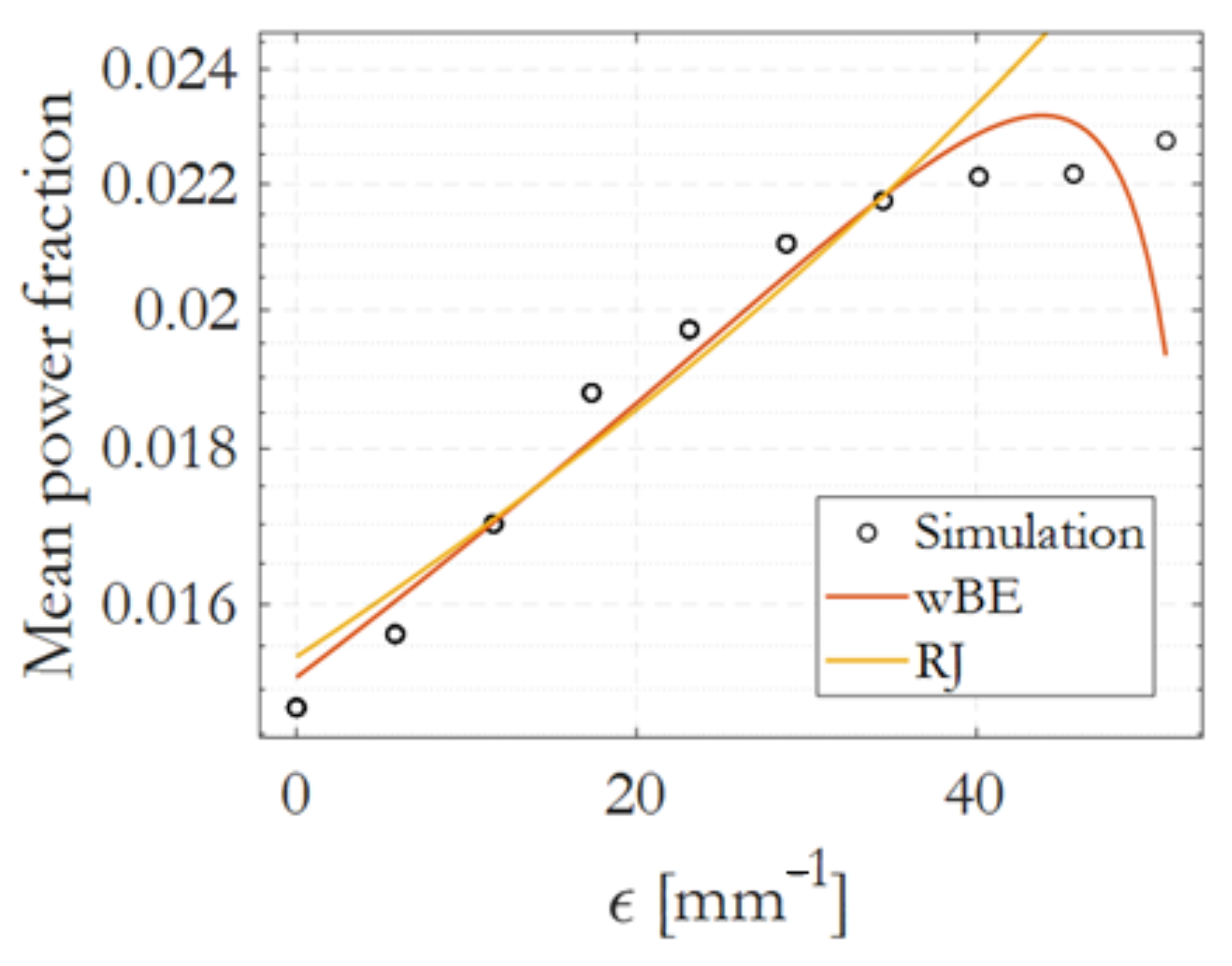
As a second case, equal power was launched over the 55 modes, obtaining the output energy distribution of Figure 6 and the mean modal power fraction of Figure 7. Also in this case, RMC caused the modal power to reach a steady state, promoting the LOMs. The mean modal power fraction | f j | 2 was properly fitted by a wBE law with T = 7.99 × 10 5 m−1, μ = 1.01 × 10 5 m−1, γ = 941 , and with a fit R-squared of 0.96 . For comparison, the data fit using an RJ was unable to represent properly the LOMs but obtained a good R-squared of 0.93 .
Recall that the simulations consider 55 modal channels of an SDM system, where each channel is composed of a pseudo-random sequence of 64 pulses at 40 Gbit/s each. This demonstrates that the RMC-induced steady states described in this work are relevant to realistic SDM systems.

3.3. Power Flow Simulation

The power-flow numerical model is an alternative to the GNLSE and is capable of describing the exchange of modal power caused by the RMC; the model treats P j as the total power propagating in modal group j and does not deal with intra-group modal coupling. The model was derived differently from the GNLSE and constitutes a valid test bed to demonstrate the formation of steady states characterized by non-uniform modal group distributions, both in the presence and absence of MDL.
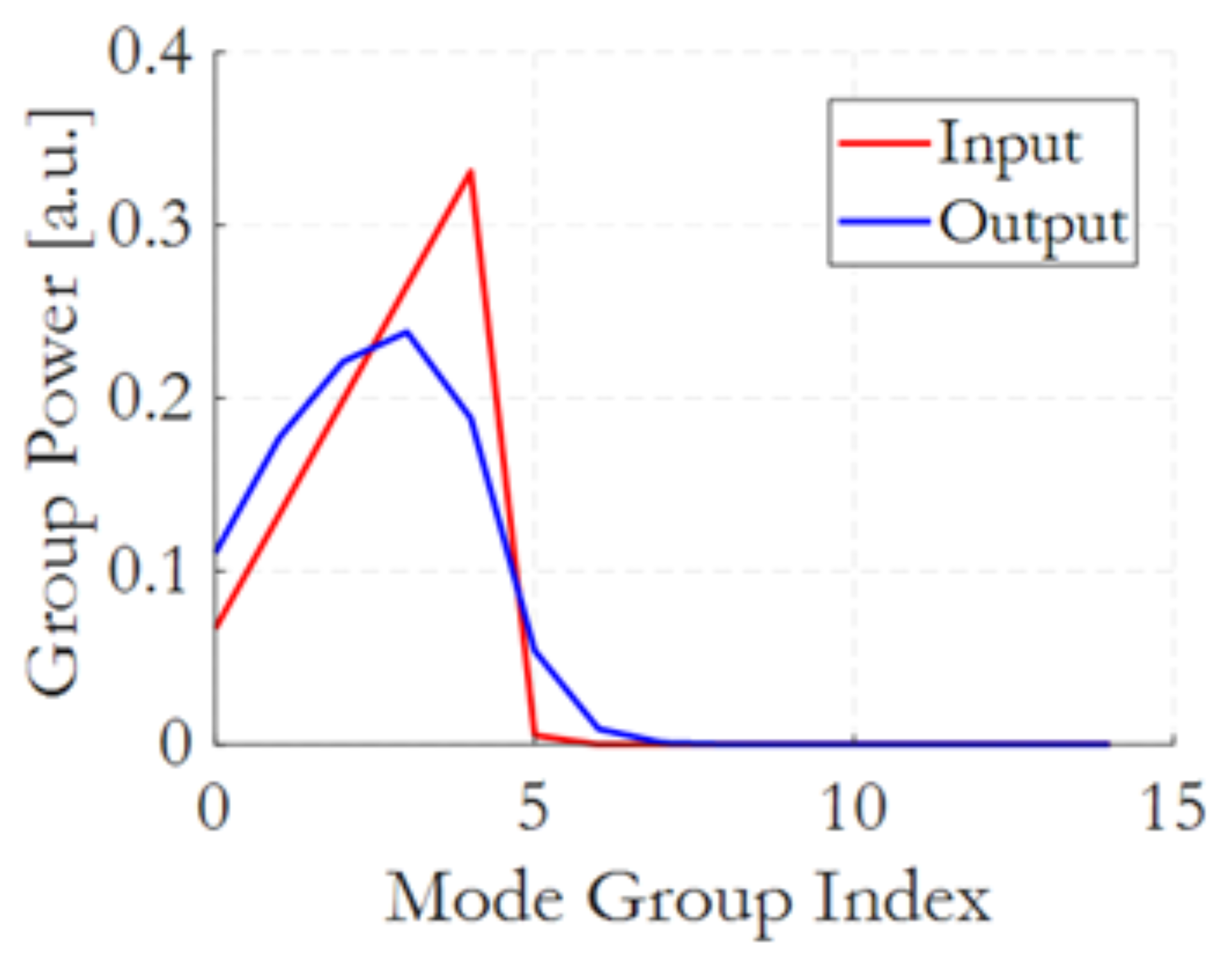
In Figure 8, equal modal power was launched in the first 5 modal groups, and no power was launched into groups 6 to 15; the input curve in the figure represents the corresponding total power in the groups. Equation (5) was used for propagation with D = 8.5 × 10 5 m−1 and A = 4.4 × 10 6 m−1. Figure shows that the output group power diffuses, promoting the LOMS. This is best highlighted in Figure 9, where it is reported the mean modal power fraction vs. eigenvalues in the presence and absence of MDL ( A = 0 ). Also in the absence of MDL, the fundamental mode carries a larger power than the modes of group 5. A wBE fit properly describes the case A = 0 , obtaining T = 1.15 × 10 7 m−1, μ = 6.24 × 10 4 m−1, γ = 12,800 and with a fit R-squared of 0.95 .

3.4. Quantum Experiment

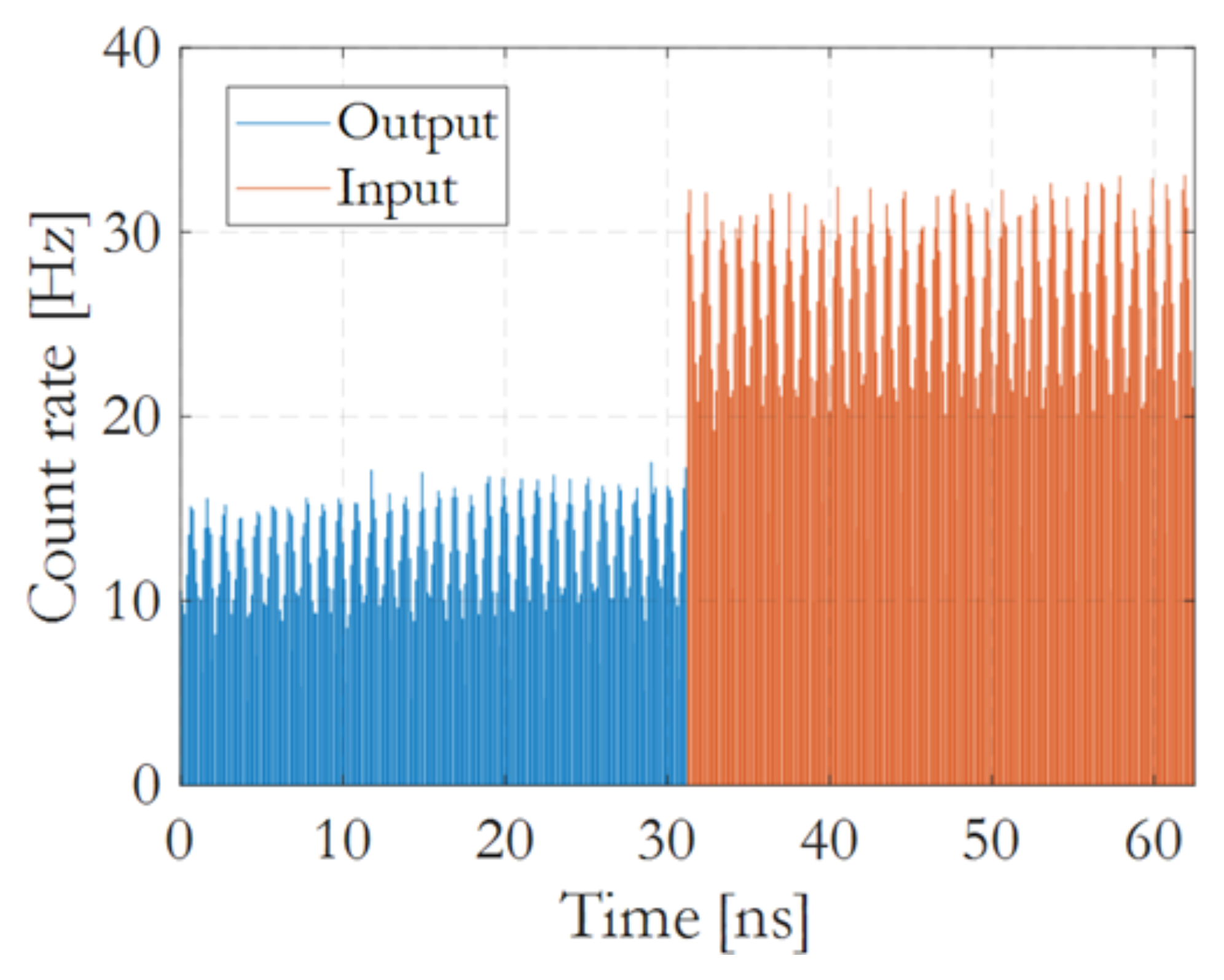
A challenging question is whether multimode fiber transmission in the quantum regime, with pulses composed of single photons, exhibits power exchange characteristics between modes similar to those observed in the linear regime. In other words, whether the RMC’s property of promoting LOMs has ergodicity characteristics. The experiment of Figure 1 was repeated after attenuating input pulses to μ = 1 photon per pulse per input mode; the same quantum power was applied to the 15 input modes and was constantly monitored at the input. Photon counts were recorded at the modal inputs and outputs by replacing the power meters with photon counting techniques, as explained in the methods section. Figure 10 is an example reporting a train of pulses at the modal inputs (in orange color) and outputs (in blue) at a repetition frequency of 1 Gpulse/s.
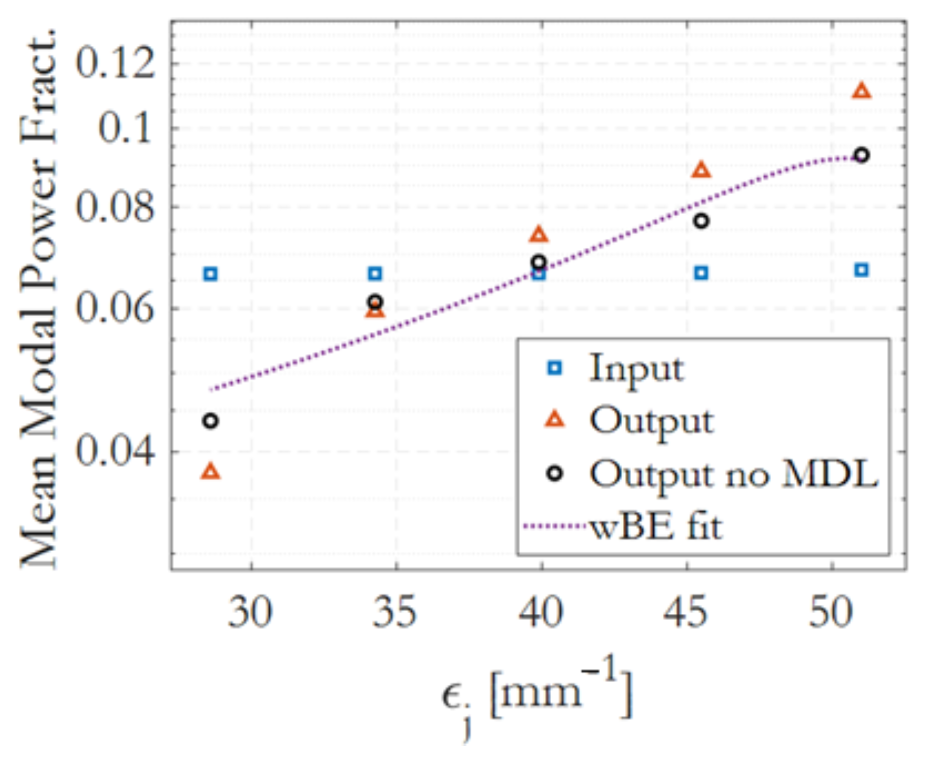
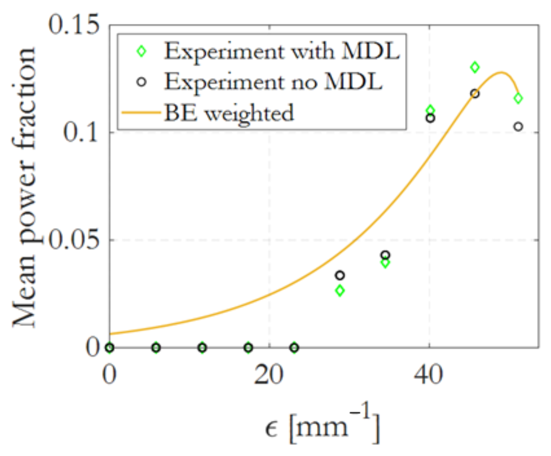
Figure 11 reports the mean (quantum) modal power fractions | f j | 2 vs. eigenvalues recorded in the first 5 modal groups, supposing the fiber supports 10 groups. Powers were obtained from output modal counts, after removing or not removing the MDL using Equation (6). The obtained quantum distribution effectively recalls the ones observed in the linear regime experiment of Figure 3 and in the simulation of Figure 7. The wBE law was able to fit the quantum distribution, obtaining T = 1.44 × 10 4 m−1, μ = 1.48 × 10 5 m−1, γ = 0.01 , and a fit R-squared of 0.97 . In the figure, empty modal groups 6 to 10 are reported by way of completeness, and are not used in the fitting process.

4. Discussion and Conclusions

All the results presented in this work, the experiment in the linear regime, numerical simulations using the coupled GNLEs, the power-flow simulations, and the experiment in the quantum regime, confirm that a sufficiently long multimode fiber produces steady state nonuniform modal distributions, even when equal power is coupled to all input modes. The MDL enhances the effect but is not the only one responsible.
The length of fiber required to produce a steady state was estimated in [24], ranging from a few hundred meters to a few kilometers depending on the magnitude of the parameter D. Consequently, it is not possible to effectively study the effects of RMC using a few meters of fiber, and it is instead necessary to precisely eliminate the effects of MDL from the experimental results.
When in steady state, the output distributions produced by the RMC alone are characterized by higher power in the LOMs and are properly fitted by the weighted Bose–Einstein law [20,21], obtaining a fit R-squared greater than 0.95. The distributions are confirmed by the experiments in the quantum regime, confirming that the RMC has ergodic properties: it is possible to obtain similar distributions measuring the optical power from multi-photon pulses or counting repeated single-photon pulses. This property paves the way for quantum thermodynamics experiments that reconcile the thermodynamics of optical multimodal systems with quantum optics.

Funding

This research was funded by Project ECS 0000024 Rome Technopole, Funded by the European Union—NextGenerationEU.

Informed Consent Statement

Not applicable.

Data Availability Statement

Data underlying the results presented in this paper are not publicly available at this time but may be obtained from the author upon reasonable request.

Conflicts of Interest

The author declares no conflicts of interest.

References

  1. Gloge, D.; Marcatili, E.A.J. Multimode theory of graded-core fibers. Bell Syst. Tech. J. 1973, 52, 1563–1578. [Google Scholar] [CrossRef]
  2. Hasegawa, A. Self-confinement of multimode optical pulse in a glass fiber. Opt. Lett. 1980, 5, 416–417. [Google Scholar] [CrossRef]
  3. Inao, S.; Sato, T.; Hondo, H.; Ogai, M.; Sentsui, S.; Otake, A.; Yoshizaki, K.; Ishihara, K.; Uchida, N. High density multicore-fiber cable. Proc. Int. Wire Cable Symp. 1979, 28, 370–384. [Google Scholar]
  4. Noordegraaf, D.; Skovgaard, P.M.W.; Nielsen, M.D.; Bland-Hawthorn, J. Efficient multi-mode to single-mode coupling in a photonic lantern. Opt. Express 2009, 17, 1988–1994. [Google Scholar] [CrossRef]
  5. Agrawal, G.P. Physics and Engineering of Graded-Index Media; Cambridge University Press: Cambridge, UK, 2023. [Google Scholar]
  6. Essiambre, R.J.; Kramer, G.; Winzer, P.J.; Foschini, G.J.; Goebel, B. Capacity Limits of Optical Fiber Networks. J. Light. Technol. 2010, 28, 662–701. [Google Scholar] [CrossRef]
  7. Winzer, P.J.; Neilson, D.T.; Chraplyvy, A.R. Fiber-optic transmission and networking: The previous 20 and the next 20 years. Opt. Express 2018, 26, 24190–24239. [Google Scholar] [CrossRef]
  8. Richardson, D.J.; Fini, J.M.; Nelson, L.E. Space-division multiplexing in optical fibres. Nat. Photonics 2013, 7, 354. [Google Scholar] [CrossRef]
  9. Gloge, D. Optical power flow in multimode fibers. Bell Syst. Tech. J. 1972, 51, 1767–1783. [Google Scholar] [CrossRef]
  10. Savović, S.; Simović, A.R.; Drljaća, B.; Djordjevich, A.; Stepniak, G.; Bunge, C.A.; Bajić, J.S. Power Flow in Graded-Index Plastic Optical Fibers. J. Light. Technol. 2019, 37, 4985–4990. [Google Scholar] [CrossRef]
  11. Ho, K.P.; Kahn, J.M. Linear Propagation Effects in Mode-Division Multiplexing Systems. J. Light. Technol. 2014, 32, 614–628. [Google Scholar] [CrossRef]
  12. Ferraro, M.; Baudin, K.; Gervaziev, M.; Fusaro, A.; Picozzi, A.; Garnier, J.; Millot, G.; Kharenko, D.; Podivilov, E.; Babin, S.; et al. Wave turbulence, thermalization and multimode locking in optical fibers. Phys. D Nonlinear Phenom. 2025, 481, 134758. [Google Scholar] [CrossRef]
  13. Berti, N.; Baudin, K.; Fusaro, A.; Millot, G.; Picozzi, A.; Garnier, J. Interplay of Thermalization and Strong Disorder: Wave Turbulence Theory, Numerical Simulations, and Experiments in Multimode Optical Fibers. Phys. Rev. Lett. 2022, 129, 063901. [Google Scholar] [CrossRef]
  14. Yadav, R.; Barbosa, F.A.; Ferreira, F.M. Modal Dynamics for Space-Division Multiplexing in Multi-Mode Fibers. J. Light. Technol. 2024, 42, 3695–3703. [Google Scholar] [CrossRef]
  15. Poletti, F.; Horak, P. Description of ultrashort pulse propagation in multimode optical fibers. J. Opt. Soc. Am. B 2008, 25, 1645–1654. [Google Scholar] [CrossRef]
  16. Wright, L.G.; Ziegler, Z.M.; Lushnikov, P.M.; Zhu, Z.; Eftekhar, M.A.; Christodoulides, D.N.; Wise, F.W. Multimode nonlinear fiber optics: Massively parallel numerical solver, tutorial, and outlook. IEEE J. Sel. Top. Quantum Electron. 2018, 24, 1–16. [Google Scholar] [CrossRef]
  17. Mumtaz, S.; Essiambre, R.J.; Agrawal, G.P. Nonlinear Propagation in Multimode and Multicore Fibers: Generalization of the Manakov Equations. J. Light. Technol. 2013, 31, 398–406. [Google Scholar] [CrossRef]
  18. Gloge, D. Bending Loss in Multimode Fibers with Graded and Ungraded Core Index. Appl. Opt. 1972, 11, 2506–2513. [Google Scholar] [CrossRef] [PubMed]
  19. Labroille, G.; Barré, N.; Pinel, O.; Denolle, B.; Lenglé, K.; Garcia, L.; Jaffrès, L.; Jian, P.; Morizur, J.F. Characterization and applications of spatial mode multiplexers based on Multi-Plane Light Conversion. Opt. Fiber Technol. 2017, 35, 93–99. [Google Scholar] [CrossRef]
  20. Zitelli, M. A New Thermodynamic Approach to Multimode Fiber Self-cleaning and Soliton Condensation. Laser Photonics Rev. 2025, 19, 2400714. [Google Scholar] [CrossRef]
  21. Zitelli, M. A Thermodynamic Approach to Linear and Quantum Cross-Talk in Multimode Fiber Systems. J. Light. Technol. 2025, 43, 3974–3981. [Google Scholar] [CrossRef]
  22. Stolen, R.H.; Tomlinson, W.J.; Haus, H.A.; Gordon, J.P. Raman response function of silica-core fibers. J. Opt. Soc. Am. B 1989, 6, 1159. [Google Scholar] [CrossRef]
  23. Wu, F.O.; Hassan, A.U.; Christodoulides, D.N. Thermodynamic theory of highly multimoded nonlinear optical systems. Nat. Photonics 2019, 13, 776–782. [Google Scholar] [CrossRef]
  24. Savović, S.; Djordjevich, A. New method for calculating the coupling coefficient in graded index optical fibers. Opt. Laser Technol. 2018, 101, 223–226. [Google Scholar] [CrossRef]
Figure 1. The experimental setup for the linear regime.
Photonics 13 00129 g001
Figure 2. Experimental output fractional modal power normalized to insertion and modal loss, when individual groups or all input modes are excited.
Photonics 13 00129 g002
Figure 3. Experimental mean modal power fraction of the output groups after uniform excitation of the input modes. A wBE fit is also shown.
Photonics 13 00129 g003
Figure 4. Simulated input and output modal energy distributions when input group 10 is launched.
Photonics 13 00129 g004
Figure 5. Average modal energy in groups 1, 5, and 10 vs. distance, in the simulation of Figure 4.
Photonics 13 00129 g005
Figure 6. Simulated input and output modal energy distributions when input modes are launched with uniform power.
Photonics 13 00129 g006
Figure 7. Mean modal power fraction vs. modal eigenvalues, for the simulation of Figure 6. A wBE and RJ fit is calculated over 10 modal groups.
Photonics 13 00129 g007
Figure 8. Input and output modal group powers simulated by the power-flow model.
Photonics 13 00129 g008
Figure 9. Mean modal power fractions vs. eigenvalues, for the simulation with uniform input power, A = 4.4 × 10 6 m−1 or A = 0 .
Photonics 13 00129 g009
Figure 10. Count rate histograms of the single-photon pulses at the input (in orange) and output (in blue) of the modal channels.
Photonics 13 00129 g010
Figure 11. Quantum mean modal power fractions | f j | 2 vs. eigenvalues recorded in the first five modal groups, with and without MDL. The wBE fit is calculated from the lossless distribution.
Photonics 13 00129 g011
Disclaimer/Publisher’s Note: The statements, opinions and data contained in all publications are solely those of the individual author(s) and contributor(s) and not of MDPI and/or the editor(s). MDPI and/or the editor(s) disclaim responsibility for any injury to people or property resulting from any ideas, methods, instructions or products referred to in the content.