Abstract
Nanostructures with the two-dimensional (2D) periodicity are attracting increasing attention due to their promising applications in planar optical devices and their potential for scalable industrial production. While Rigorous Coupled-Wave Analysis (RCWA) has proven to be an efficient electromagnetic solver for simulating the diffraction of large-scale periodic nanostructures, it has been largely applied in nanostructures with one-dimensional (1D) periodicity and suffers from potentially low computational stability. In this study, we present a step-by-step formulation of the RCWA algorithm for 2D stratified grating structures. Through dimensionality reduction, we show that the boundary conditions in 2D gratings can be transformed into forms analogous to those of 1D gratings. Additionally, we implement a hybrid matrix algorithm to enhance the computational stability of the RCWA. The stability and accuracy of the hybrid matrix-enhanced RCWA algorithm are compared with other recursive methods. An exemplary application in metalens demonstrates the effectiveness of our algorithms.
1. Introduction
Being a type of two-dimensional (2D) periodic structure, metasurfaces have emerged as a versatile tool for controlling light at the nanoscale [1,2,3]. These periodic subwavelength nanostructures enable the unprecedented manipulation of the phase [4], amplitude [5], and polarization [6] of electromagnetic waves, paving the way for compact and high-performance optical devices [7,8,9,10]. Two-dimensional gratings are one kind of metasurfaces, which pattern the nanostructures periodically in the two directions of the in-plane. They have garnered increasing attention from researchers due to the development of nanofabrication technologies [11]. For the analysis of such 2D periodic structures, several computational approaches are commonly employed, such as Finite-Difference Time Domain [12], boundary element method (BEM) [13,14], the Finite Element Method [15], and Rigorous Coupled-Wave Analysis (RCWA) [16,17,18,19,20]. As a semi-analytical electromagnetic solver, RCWA has the advantages over other approaches of both accuracy and efficiency if a large area (cm2 or beyond) of nanostructures is required [11]. For example, the cutting-edge augmented-reality glasses based on diffractive optical elements [21] and the inversely designed [22,23] optical devices usually require numerous computational resources for full-wave simulations, making other numerical approaches almost impossible.
Tamir, Wang, and Oliver [24] appear to have first applied the RCWA to grating problems in the mid-1960s. From 1981 to 1986, Moharam and Gaylord used the RCWA to analyze slanted gratings [25], conical gratings [26], and metallic gratings [27]. In 1996, Lalanne and Morris proposed a novel formulation that significantly enhanced the convergence rates for TM polarization in 1D gratings [17]. Following this work, Lalanne introduced a new formula applicable to 2D gratings [18]. In 1996, Li established a theoretical framework [19] that showed that the reason for the success of Lalanne’s formulation [17] was that it uniformly preserved the continuity of appropriate field components across the discontinuities of the permittivity function. In 1997, Li presented a new formulation [20] of the RCWA that applies correct rules [19] of Fourier factorization for crossed surface-relief gratings. RCWA with such a Fourier factorization converged much faster than traditional approaches. In 2003, Li introduced formulas for crossed anisotropic gratings featuring arbitrary permittivity and permeability tensors [28]. In 2008, Liu and Lalanne developed an RCWA algorithm to discuss 2D metallic gratings, focusing on extraordinary optical transmission (EOT) through subwavelength nanohole arrays [29]. In 2005, Logofatu developed a methodological framework that integrated analytical formulations with computational implementation for 2D gratings [30]. In recent years, several ideas for RCWA algorithms without solving eigenvalues have been progressively proposed [31,32]. While RCWA for single-layer gratings is well-established, its numerical instability in matching boundary conditions across multilayered grating interfaces has become a focal point of the research.
To tackle the computational instability and inefficiency for large-depth gratings, Moharam et al. [33] proposed the enhanced transmittance matrix (T-matrix) method for the stratified structures of 1D gratings. Compared to the standard T-matrix algorithm, the enhanced algorithm effectively reduces computational instability. Apart from the enhanced T-matrix method widely used in optics, other methods, including the reaction matrix (R-matrix) [34] and scattering matrix (S-matrix) [35], were put forward to enhance the computational stability of RCWA for stratified 1D gratings. In 2006, Tan presented enhanced R-matrix algorithms, which delivered superior stability compared to conventional R-matrix algorithms [36]. In 2011, Rumpf proposed an enhanced S-matrix algorithm by sandwiching a grating layer between two virtual thicknessless vacuum layers, accelerating the computational time by potential parallel processes [37]. Tan [38] pointed out that the T-matrix and R-matrix methods might exhibit sever computational instabilities if the thickness of the grating layer becomes excessively large or small, respectively. He proposed a so-called hybrid matrix (H-matrix) method for grating structures with an arbitrary thickness but with 1D periodicity. The H-matrix method demonstrated superior stability over the T-matrix and R-matrix methods [38].
In comparison with the 1D case, the computational stability problem of RCWA for structures with 2D periodicity is more severe considering the increased electromagnetic mode coupling complexity, but has received much less attention. In this work, the RCWA algorithms for the structures with 2D periodicity are derived step by step. Through systematic numerical benchmarking, we demonstrate the superior performance of the enhanced H-matrix relative to widely adopted large-scale computation matrices. The results confirm its optimal stability and computational efficiency as a boundary matching algorithm for reflection analysis. We used the design of metalens, for example, to demonstrate the application of such algorithms.
2. Formulation
2.1. Fourier Expansion of the Permittivity Within the Grating Region
A plane wave with wavelength λ is incident with an incidence angle θ, an azimuth angle ϕ, and a polarization angle ψ. The definition of the angles and the geometry of grating are shown in Figure 1a. The grating is bound by two semi-infinitive homogeneous media, Region I and Region II, with relative permittivity values of εI and εII, respectively. The relative permeability for the three regions is μ = 1. The 2D grating exhibits a spatial period of Λx along the x-axis and Λy along the y-axis. As Figure 1b shows, the grating has alternating regions of dielectric constants, εrd (ridge) and εgr (groove); the dielectric permittivity can be represented as [30]:
where fx = fx2 − fx1, fy = fy2 − fy1. fx1, fx2 represent the dimensionless fractions of the two boundaries of a grating ridge with respect to a grating period along the x-axis. fy1, and fy2 have the same indications, but along the y-axis. The dielectric function in the grating region is first expanded using a Fourier series, which can be expressed as [30]:
where εmn is the (m, n)th Fourier coefficient of the relative permittivity. Kx and Ky are defined as Kx=2π/Λx, Ky=2π/Λy. The coefficients of the Fourier expansion (2) can be calculated by:
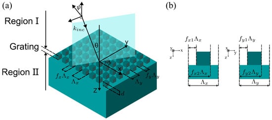
Figure 1.
(a) Schematics of single 2D-layer grating structures. (b) Schematic diagram of unit 2D grating structures.
According to Li [20], the algorithm demonstrated significantly accelerated convergence when utilizing the following Fourier decomposition.
where:
2.2. Electromagnetic Fields at Region I and Region II
The incident electric field can be expressed as [28]:
where σ = x, y, or z, representing the electric component along the x-, y-, or z- direction. is the amplitude of the incident electric field. The , , can be defined as [30]:
where is defined as the wave number in Region I. is defined as the wave number in Region II. Then, electric fields in Region I and Region II are expressed with the following Rayleigh expansions [20]:
where σ = x or y. and are the amplitudes of the (m, n)th-order reflected and transmitted electric fields, respectively. and are defined as:
is to be solved from:
where a = I or II, which represents the wave number in Region or Region . The sign of is chosen according to [28]:
The Maxwell’s equations, when utilizing Gaussian units, are given by the following equations [28]:
where k0 = 2π/λ is the wave number in the vacuum. In Region I and Region II, by substituting Equations (10) and (11) into Maxwell’s Equation (14), the amplitudes of electromagnetic fields in Region II and Region I can be written as [28]:
where , , and are defined as [28]:
The reason for writing the electromagnetic fields in the form of Equation (15) is that the field components share a similar configuration for the three regions, as will be discussed in the subsequent sections in this paper.
2.3. Electromagnetic Fields at the Grating Region
The electromagnetic fields can be expressed using a Fourier expansion in the grating region, which can be written as [30]:
where , , , and are the complex amplitudes of the electromagnetic field. By substituting Equations (20) and (21) into Maxwell’s Equation (14), the spatial harmonic components within the grating region are derived [30]:
To unify the dimensionality of all the variables, the indices for the 2D grating are redefined as:
where s1 = 2nmax + 1 and s2 = 2hmax + 1. Here, m ranges from −mmax to mmax, n ranges from–nmax to nmax, p ranges from −pmax to pmax, and h ranges from −hmax to hmax, with mmax = pmax and nmax = hmax. The parameters mmax and pmax represent the maximum order of Fourier harmonics in the x-axis. Similarly, nmax and hmax represent the maximum order of Fourier harmonics in the y-axis. Thus, the index u ranges from −mmax (2nmax + 1) − nmax to mmax (2nmax + 1) +nmax, and v ranges from −pmax (2hmax + 1) − hmax to pmax (2hmax + 1) + hmax. The total number of possible values for u is (2mmax + 1) (2nmax + 1), and for v, it is (2pmax + 1) (2hmax + 1). When mmax = pmax = 0(nmax = hmax = 0) and fx = 1(fy = 1), the 2D grating turns into a 1D grating with the periodicity in the y- (x-) axis. The dimensionality reduction from 4D to 2D is achieved by Ξuv = εm-p,n-h, Auv = 1/εm-p,n-h, =, =. The wave vectors are converted to 2D vectors via the following diagonal matrix construction: , . δuv is the Kronecker delta function, which is zero everywhere, except u = v.
After unifying the dimensionality of all the variables, Equations (22)–(25) can be reduced to:
According to Li [20], the convergence is significantly improved when and are defined as:
Equation (27) can be further reduced to:
where M = F*G. The coupled-wave Equation (30) can be addressed by determining the eigenvectors and the eigenvalues associated with the matrix M. Following this, the amplitudes of the electric and magnetic fields in the grating region can be expressed as [28]:
Q and W are the eigenvalue and eigenvector matrices of the matrix M, respectively. quvj and Wσuvj are the elements of matrices and W, respectively. The sign of the quvj should be satisfied to [20]:
V = GW/(k0Q). and can be determined by matching boundary conditions. Equations (31) and (32) can be expressed as a matrix form:
Equation (34) can be further simplified as:
where
Employing an identical transformation, Equation (15) can be recast in an equivalent structure. Equation (35) is analogous to the RCWA formulas for 1D gratings, where W and V are the eigenvector matrix blocks. X is the propagation matrix block. c+ and c− represent unknown constants in different regions, which are determined by applying boundary condition matching.
2.4. Matching the Boundary Conditions in Single-Layer 2D Gratings
To determine the unknown constants, we first considered matching the boundary conditions for the single layer of gratings. The relationship of electromagnetic fields between z = 0 and z = d can be expressed in an H-matrix form [38]:
where matrix blocks H[1] can be obtained from:
W and V are the eigenvector matrix blocks in the single grating layer. X is the propagation matrix in the single grating layer. Now, we match the tangential electric and magnetic fields through [38]:
For most grating problems, transmission and reflection amplitudes are expected, which can be obtained by [38]:
Once the diffraction amplitudes are obtained from Equation(39), the diffraction efficiencies can be determined by using [28]:
where , and are can be derived by through Equations (16) and (26). , , and are defined as:
2.5. Matching the Boundary Conditions in Stratified 2D Gratings
For stratified 2D gratings, as shown in Figure 2, the grating region is further divided into L layers. The refraction index of the lth layer is nl (l = 1, 2, …, L) and the thickness of the lth layer is dl. Each layer may have distinct a grating period or filling factor. There are connections between the electromagnetic field at the boundaries z = Zl− and z = ZL+, which can be described using a stacked H[l] matrix:
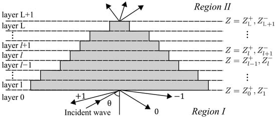
Figure 2.
Schematics of a stratified unit grating cell.
The relationship between stack H[l] and stack H[l+1] is [38]:
H[L+1] is the H-matrix of the output layer, which is:
By substituting Equation (44) into Equation (43), the H[L] matrix at layer L can be obtained from the H[L+1] matrix at layer L+1. Substituting H[L] into Equation (43) yields H[L−1]. By repeating this procedure, H[1] is ultimately acquired. H[1] provides the connection of electromagnetic fields between the first layer and L layer. After obtaining H[1], for stratified grating structures, the transmission and reflection amplitudes, as well as the diffraction amplitudes, can be calculated using Equations (39)–(41).
For problems solely concerning reflectance, the enhanced H matrix is expressed by [38]:
where:
We assume the layer is infinite, so is determined by:
The reflection efficiency is given by [38]:
The enhanced H matrix exhibits greater stability than other algorithms. A detailed discussion is provided in the next section.
3. Numerical Result
For numerical validations, we first verify the stability of the enhanced H-matrix method using a symmetric single-layer 2D grating. The incident wavelength λ is 1 μm. The incident angle, azimuth angle, and polarization angle are set as θ = ϕ = ψ = 0°. The key parameters of the grating are listed in Table 1.

Table 1.
The parameter of the symmetric single-layer grating.
Figure 3 compares computational stability as a function of grating thickness d between five algorithms, the T-matrix (circles), S-matrix (dashed line), R-matrix (square), H-matrix (triangular), and enhanced H-matrix (solid line), in a logarithmic coordinate system. The condition number of a matrix is the ratio between the largest singular value and the smallest singular value, implying the sensitivity of output values to the input data. A larger condition number indicates greater matrix instability and a higher likelihood of numerical errors during matrix inversion. We calculated the condition numbers of the matrices to be inverted in these methods. For instance, the condition number of the matrix to be inverted in H[1] corresponds to the condition number of the second matrix on the right-hand side of Equation (43). We calculated the condition numbers in T[1] (Equation (16) in Ref. [38]), R[1] (Equation (17) in Ref. [36]), S[1] (Equation (19) in Ref. [37]), H[1] (Equation (32)), and enhanced H[1] (Equation (45)) versus the layer thickness relative to the wavelength.
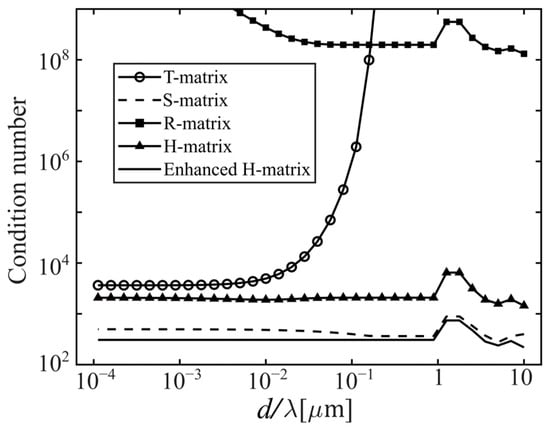
Figure 3.
Comparison of the condition numbers between five recursive methods.
As Figure 3 shows, the condition numbers in R[1] decrease as the grating thickness increases in the bilogarithmic diagram, indicating the R-matrix method is suitable for the thick gratings. By contrast, the condition numbers in T[1] increase almost exponentially as the grating thickness increases, meaning that the T-matrix method is suitable for the thin gratings. However, the H-matrix and S-matrix combine the advantages of the R-matrix method and T-matrix method. The condition numbers of H[1] and S[1] to be inverted initiate from a much lower level than R and remain quite stable for a large thickness range. Notably, condition numbers in enhanced H[1] to be inverted demonstrate the smallest value compared to the other methods, which demonstrates unconditional computational stability, even for 2D periodic structures.
To evaluate computational efficiency, an asymmetric single-layer 2D grating was used for comparative analysis. Table 2 lists the details of the testing platform. It can be noted that all the benchmarks are evident on the same platform. The incident wavelength λ is 1 μm. The angles of incidence, azimuth, and polarization are all set to θ = ϕ = ψ = 0°. Parameters are detailed in Table 3. Harmonic orders—representing the maximum Fourier expansion terms in RCWA simulations—directly influence solution accuracy. While higher harmonics improve precision, they increase computational demands. We employed both the enhanced H-matrix and the S-matrix method to compute reflection coefficients for this structure, with the computation time serving as the efficiency metric. The runtime measurement method uses MATLAB R2022a’s tic and toc functions, while memory usage is measured with MATLAB’s memory function. These functions collect the memory usage and time consumption of the S-matrix and H-matrix code blocks, while the memory usage and time consumption of other code blocks, such as eigenvector calculations, are not included. As Figure 4a shows, the enhanced H-matrix method consistently outperforms the S-matrix approach, reducing the computation time by a range of 16–30%. According to Figure 4b, the enhanced H-matrix outperforms the S-matrix, with a memory consumption value reduced by approximately 20%. This indicates that the enhanced H-matrix shows advantages in optimizing memory usage as well as in computational efficiency. It should be noted that during the computation of the S-matrix, transmission-related variables were intentionally excluded—only reflection variables were computed—ensuring a valid comparison.
Table 2.
The detailed implementation and testing setup information.
Table 3.
The parameter of the asymmetric single-layer grating.

Figure 4.
(a) Comparison of the computational speed between the S-matrix and enhanced H-matrix. (b) Comparison of the memory usage between the S-matrix and enhanced H-matrix.
We next verify the accuracy of the H-matrix using three-layer grating slabs, as shown in Figure 5a. The light is incident from Region II. The incident wavelength is 1.55 µm, with incident angles of θ = 0°, ϕ = 0°, and ψ = 0°. The grating parameters are listed in Table 4. Figure 5b shows the simulation results using the S-matrix method (cube and triangle symbols) and H-matrix method (cross and dashed line). The x-axis represents the first layer thickness relative to the wavelength, and the y-axis shows reflection and transmission efficiencies. When the normalized parameter d1/λ is relatively small, variations in d1 are minimal; consequently, diffraction efficiency shows only minor changes. Conversely, when d1/λ is sufficiently large, variations in d1 become substantial, resulting in significant alterations in the diffraction efficiency. As can be seen, there is a good agreement between the H-matrix method and S-matrix method, validating the accuracy of our proposed H-matrix algorithm. In Figure 5b, the solid line represents the results of the enhanced H-matrix algorithm. The enhanced H-matrix method provides almost the same results as those of the regular H-matrix method and S-matrix method, but the required computation memory is reduced by almost half [38].
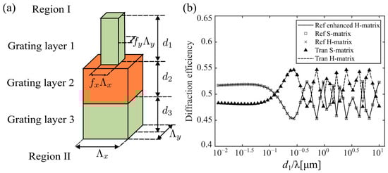
Figure 5.
(a) Schematic unit cell of a three-layer grating slabs. (b) Validation of H-matrix computational accuracy against the S-matrix method.
Table 4.
Three-layer grating slabs.
We finally demonstrate the practical application of such an H-matrix-enhanced 2D RCWA algorithm. To validate the algorithm, a metalens consisting of 2D gratings was designed. The incident light with a wavelength of 532 nm is normally incident at θ = ϕ = ψ = 0° on the metalens. The unit cell of the metalens comprises a substrate layer with a thickness of 1 μm and a refractive index of 1.5. The nanopillar within the unit cell of the metalens has a refractive index of 2.04 and a height of 1.2 μm. The periodicity of the unit structure is 0.45 μm. As shown in Figure 6a, a parametric database was established utilizing the 2D RCWA H-matrix algorithm. The database established a map between Pw and the phase of transmission. Pw denotes the cross-sectional width of the cube-shaped nanopillar. According Capasso [39], the metalens unit cells are spatially arranged according to hyperbolic phase requirements. The metalens is designed with a focal length of 100 μm and a radius of 11 μm. An approximate method was employed to compute electromagnetic fields in the far-field beyond the metalens [3]. The distribution of electric field intensity in the x-z plane is shown in Figure 6b. Figure 6c shows the electric field amplitude along the x-direction in the focal plane. The full-width at half maximum of the focus is 2.35 μm. The results demonstrate that the metalens designed using the 2D RCWA H-matrix algorithm achieves excellent phase matching, thereby validating the accuracy of our algorithm.
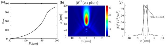
Figure 6.
The metalens is designed using the 2D RCWA H-matrix algorithm. (a) The database establishing a map between Pw and the phase of transmission. (b) Simulated electric field in the x-z cross-section. (c) Electric field intensity in the focal plane.
4. Conclusions
In this paper, we derive the RCWA algorithms for 2D gratings step by step. We also develop a stable enhanced H-matrix algorithm for 2D stratified grating structures. The simulation results of specific grating structures demonstrate that the enhanced H-matrix algorithm offers better stability compared to the T-matrix, R-matrix and S-matrix algorithms. The integration of the enhanced H-matrix with 2D grating structures provides a more stable and efficient approach. Notably, the dimensionality reduction achieved through the enhanced matrix methodology offers a new solution to address the prolonged runtime and excessive memory consumption in the inverse designs of metasurfaces, which will be an interesting research topic in our future study.
Author Contributions
K.S.: Conceptualization, Data Curation, Formal Analysis, Investigation, Methodology, Software, Validation, Visualization, Writing—Original Draft Preparation, and Writing—Review and Editing; J.W.: Conceptualization, Data Curation, Formal Analysis, Investigation, Methodology, Resources, Validation, Writing—Original Draft Preparation, Writing—Review and Editing, Funding Acquisition, and Supervision; G.W.: Methodology, Validation, Writing—Review and Editing, and Supervision. All authors have read and agreed to the published version of the manuscript.
Funding
J.W. gratefully acknowledges the General Program of the Natural Science Foundation of China (62475065) and the Scientific Research Starting Fund received from Hangzhou Dianzi University (GK239909299001-408, KYS045623025).
Data Availability Statement
Data underlying the results presented in this paper are not publicly available at this time but may be obtained from the authors upon reasonable request.
Conflicts of Interest
The authors declare no conflicts of interest.
References
- Yu, N.; Capasso, F. Flat optics with designer metasurfaces. Nat. Mater. 2014, 13, 139–150. [Google Scholar] [CrossRef]
- Yu, N.; Genevet, P.; Kats, M.A.; Aieta, F.; Tetienne, J.-P.; Capasso, F.; Gaburro, Z. Light propagation with phase discontinuities: Generalized laws of reflection and refraction. Science 2011, 334, 333–337. [Google Scholar] [CrossRef] [PubMed]
- Pestourie, R.; Pérez-Arancibia, C.; Lin, Z.; Shin, W.; Capasso, F.; Johnson, S.G. Inverse design of large-area metasurfaces. Opt. Express 2018, 26, 33732–33747. [Google Scholar] [CrossRef]
- Aieta, F.; Kats, M.A.; Genevet, P.; Capasso, F. Multiwavelength achromatic metasurfaces by dispersive phase compensation. Science 2015, 347, 1342–1345. [Google Scholar] [CrossRef]
- Lee, G.-Y.; Yoon, G.; Lee, S.-Y.; Yun, H.; Cho, J.; Lee, K.; Kim, H.; Rho, J.; Lee, B. Complete amplitude and phase control of light using broadband holographic metasurfaces. Nanoscale 2018, 10, 4237–4245. [Google Scholar] [CrossRef]
- Zhao, Y.; Alù, A. Manipulating light polarization with ultrathin plasmonic metasurfaces. Phys. Rev. B 2011, 84, 205428. [Google Scholar] [CrossRef]
- Khorasaninejad, M.; Chen, W.T.; Devlin, R.C.; Oh, J.; Zhu, A.Y.; Capasso, F. Metalenses at visible wavelengths: Diffraction-limited focusing and subwavelength resolution imaging. Science 2016, 352, 1190–1194. [Google Scholar] [CrossRef] [PubMed]
- Wang, J.; Coillet, A.; Demichel, O.; Wang, Z.; Rego, D.; Bouhelier, A.; Grelu, P.; Cluzel, B. Saturable plasmonic metasurfaces for laser mode locking. Light Sci. Appl. 2020, 9, 50. [Google Scholar] [CrossRef]
- Zhang, L.; Sun, X.; Yu, H.; Deng, N.; Qiu, F.; Wang, J.; Qiu, M. Plasmonic metafibers electro-optic modulators. Light Sci. Appl. 2023, 12, 198. [Google Scholar] [CrossRef] [PubMed]
- Zhang, C.; Zhang, L.; Zhang, H.; Fu, B.; Wang, J.; Qiu, M. Pulsed polarized vortex beam enabled by metafiber lasers. PhotoniX 2024, 5, 36. [Google Scholar] [CrossRef]
- Dainese, P.; Marra, L.; Cassara, D.; Portes, A.; Oh, J.; Yang, J.; Palmieri, A.; Rodrigues, J.R.; Dorrah, A.H.; Capasso, F. Shape optimization for high efficiency metasurfaces: Theory and implementation. Light Sci. Appl. 2024, 13, 300. [Google Scholar] [CrossRef] [PubMed]
- Yee, K. Numerical solution of initial boundary value problems involving Maxwell’s equations in isotropic media. IEEE Trans. Antennas Propag. 1966, 14, 302–307. [Google Scholar] [CrossRef]
- García de Abajo, F.J.; Howie, A. Retarded field calculation of electron energy loss in inhomogeneous dielectrics. Phys. Rev. B 2002, 65, 115418. [Google Scholar] [CrossRef]
- Hohenester, U.; Trügler, A. MNPBEM—A Matlab toolbox for the simulation of plasmonic nanoparticles. Comput. Phys. Commun. 2012, 183, 370–381. [Google Scholar] [CrossRef]
- Jin, J.-M. The Finite Element Method in Electromagnetics, 3rd ed.; John Wiley & Sons: Hoboken, NJ, USA, 2015. [Google Scholar]
- Moharam, M.G.; Grann, E.B.; Pommet, D.A.; Gaylord, T.K. Formulation for stable and efficient implementation of the rigorous coupled-wave analysis of binary gratings. J. Opt. Soc. Am. A 1995, 12, 1068–1076. [Google Scholar] [CrossRef]
- Lalanne, P.; Morris, G.M. Highly improved convergence of the coupled-wave method for TM polarization. J. Opt. Soc. Am. A 1996, 13, 779–784. [Google Scholar] [CrossRef]
- Lalanne, P. Improved formulation of the coupled-wave method for two-dimensional gratings. J. Opt. Soc. Am. A 1997, 14, 1592–1598. [Google Scholar] [CrossRef]
- Li, L. Use of Fourier series in the analysis of discontinuous periodic structures. J. Opt. Soc. Am. A 1996, 13, 1870–1876. [Google Scholar] [CrossRef]
- Li, L. New formulation of the Fourier modal method for crossed surface-relief gratings. J. Opt. Soc. Am. A 1997, 14, 2758–2767. [Google Scholar] [CrossRef]
- Zhao, J.; Tian, X.; Wang, J. Conical diffractions of multilayered gratings modeled by Cartesian rigorous coupled-wave analysis. J. Opt. Soc. Am. A 2023, 40, 1940–1946. [Google Scholar] [CrossRef]
- Liu, V.; Fan, S. S4: A free electromagnetic solver for layered periodic structures. Comput. Phys. Commun. 2012, 183, 2233–2244. [Google Scholar] [CrossRef]
- Sapra, N.V.; Vercruysse, D.; Su, L.; Yang, K.Y.; Skarda, J.; Piggott, A.Y.; Vučković, J. Inverse design and demonstration of broadband grating couplers. IEEE J. Sel. Top. Quantum Electron. 2019, 25, 6100207. [Google Scholar] [CrossRef]
- Tamir, T.; Wang, H.C.; Oliner, A.A. Wave propagation in sinusoidally stratified dielectric media. IEEE Trans. Microw. Theory Tech. 1964, 12, 323–335. [Google Scholar] [CrossRef]
- Moharam, M.G.; Gaylord, T.K. Rigorous coupled-wave analysis of planar-grating diffraction. J. Opt. Soc. Am. 1981, 71, 811–818. [Google Scholar] [CrossRef]
- Moharam, M.G.; Gaylord, T.K. Three-dimensional vector coupled-wave analysis of planar-grating diffraction. J. Opt. Soc. Am. 1983, 73, 1105–1112. [Google Scholar] [CrossRef]
- Moharam, M.G.; Gaylord, T.K. Rigorous coupled-wave analysis of metallic surface-relief gratings. J. Opt. Soc. Am. A 1986, 3, 1780–1787. [Google Scholar] [CrossRef]
- Li, L. Fourier modal method for crossed anisotropic gratings with arbitrary permittivity and permeability tensors. J. Opt. A Pure Appl. Opt. 2003, 5, 345. [Google Scholar] [CrossRef]
- Liu, H.; Lalanne, P. Microscopic theory of the extraordinary optical transmission. Nature 2008, 452, 728–731. [Google Scholar] [CrossRef]
- Logofatu, P.C. Rigorous coupled-wave analysis for two-dimensional gratings. Proc. SPIE 2005, 5972, 59720Q. [Google Scholar] [CrossRef]
- Li, J.; Shi, L.; Ma, Y.; Ran, Y.; Liu, Y.; Wang, J. Efficient and stable implementation of RCWA for ultrathin multilayer gratings: T-matrix approach without solving eigenvalues. IEEE Antennas Wirel. Propag. Lett. 2020, 20, 83–87. [Google Scholar] [CrossRef]
- Xu, J.; Charlton, M.D.B. Highly efficient Rigorous Coupled-Wave Analysis implementation without eigensystem calculation. IEEE Access 2024, 12, 127966–127975. [Google Scholar] [CrossRef]
- Moharam, M.G.; Pommet, D.A.; Grann, E.B.; Gaylord, T.K. Stable implementation of the rigorous coupled-wave analysis for surface-relief gratings: Enhanced transmittance matrix approach. J. Opt. Soc. Am. A 1995, 12, 1077–1086. [Google Scholar] [CrossRef]
- Li, L. Multilayer modal method for diffraction gratings of arbitrary profile, depth, and permittivity. J. Opt. Soc. Am. A 1993, 10, 2581–2591. [Google Scholar] [CrossRef]
- Li, L. Formulation and comparison of two recursive matrix algorithms for modeling layered diffraction gratings. J. Opt. Soc. Am. A 1996, 13, 1024–1035. [Google Scholar] [CrossRef]
- Tan, E.L. Enhanced R-matrix algorithms for multilayered diffraction gratings. Appl. Opt. 2006, 45, 4803–4809. [Google Scholar] [CrossRef]
- Rumpf, R.C. Improved formulation of scattering matrices for semi-analytical methods that is consistent with convention. Prog. Electromagn. Res. B 2011, 35, 241–261. [Google Scholar] [CrossRef]
- Tan, E.L. Hybrid-matrix algorithm for rigorous coupled-wave analysis of multilayered diffraction gratings. J. Mod. Opt. 2006, 53, 417–428. [Google Scholar] [CrossRef]
- Chen, W.T.; Zhu, A.Y.; Sanjeev, V.; Khorasaninejad, M.; Shi, Z.; Lee, E.; Capasso, F. A broadband achromatic metalens for focusing and imaging in the visible. Nat. Nanotechnol. 2018, 13, 220–226. [Google Scholar] [CrossRef] [PubMed]
Disclaimer/Publisher’s Note: The statements, opinions and data contained in all publications are solely those of the individual author(s) and contributor(s) and not of MDPI and/or the editor(s). MDPI and/or the editor(s) disclaim responsibility for any injury to people or property resulting from any ideas, methods, instructions or products referred to in the content. |
© 2025 by the authors. Licensee MDPI, Basel, Switzerland. This article is an open access article distributed under the terms and conditions of the Creative Commons Attribution (CC BY) license (https://creativecommons.org/licenses/by/4.0/).