Article

A CNN-GS Hybrid Algorithm for Generating Pump Light Fields in Atomic Magnetometers

1
School of Instrumentation and Optoelectronic Engineering, Beihang University, Beijing 100191, China
2
Zhejiang Provincial Key Laboratory of Ultra-Weak Magnetic-Field Space and Applied Technology, Hangzhou Innovation Institute, Beihang University, Hangzhou 310051, China
3
Hangzhou Institute of Extremely-Weak Magnetic Field Major National Science and Technology Infrastructure, Beihang University, Hangzhou 310051, China
4
Hefei National Laboratory, Hefei 230088, China
*
Authors to whom correspondence should be addressed.
Photonics 2025, 12(8), 796; https://doi.org/10.3390/photonics12080796
Submission received: 27 June 2025 / Revised: 29 July 2025 / Accepted: 5 August 2025 / Published: 7 August 2025

Abstract

Atomic magnetometers (AMs), recognized for their ultra-high magnetic sensitivity, demand highly uniform pump light fields to maximize measurement accuracy. In this paper, a phase modulation-based method using convolutional neural networks (CNN) and the Gerchberg–Saxton (GS) algorithm is proposed to generate the pumping light field, and the model was trained using a supervised learning approach with a custom dataset. The specific training settings are as follows: the backpropagation algorithm was adopted as the training algorithm, and the Adam optimization method was used for network training, with a learning rate of 0.001 and a total of 100 training epochs, utilizing a liquid crystal spatial light modulator (LCSLM) to regulate the light field phase distribution dynamically. By transforming Gaussian beams into flat-top beams, the method significantly enhances polarization uniformity within vapor cells, leading to improved magnetometric sensitivity. The proposed hybrid algorithm reduces the mean square error from 35% to 19% and peak non-uniformity from 21% to 7.6%. A reflective LCSLM-based optical setup is implemented to produce circular and square flat-top beams with a measured non-uniformity of 5.1%, resulting in an enhancement of magnetic sensitivity from 14.04 fT/Hz1/2 to 7.80 fT/Hz1/2.

1. Introduction

Quantum precision measurement technology can be widely applied to research such as frontier physics exploration [1], magnetic anomaly detection [2], space magnetic field detection [3], biological magnetic field detection [4], and resource exploration [5]. With the development of quantum technology and laser technology, the spin-exchange relaxation-free (SERF) atomic magnetometer (AM) has become a research hotspot in the field of ultra-sensitive extremely weak magnetic field detection [6,7,8,9], which will enable magnetic field measurements at the a T (10−18 T) magnitude level in the future [10]. In particular, AM possesses the advantages of easy miniaturization and wearability and has no need for liquid nitrogen cooling, thus holding significant research and application value in human magnetic field measurements such as magnetoencephalography (MEG) and magnetocardiography (MCG) [11,12,13,14,15].
The SERF AM is a high-precision measurement sensor that detects weak magnetic fields by measuring the spin effects of alkali metal atoms in a SERF state [16,17,18]. It polarizes alkali metal atoms through optical pumping and measures changes in laser polarization or absorption characteristics caused by Larmor precession induced by external magnetic fields to determine the magnetic field strength [19,20]. Therefore, the quality of the laser beam directly impacts atomic polarization and dynamic response detection. The Gaussian laser spot output by the laser enters the sensor’s vapor cell to polarize alkali metal atoms. However, Gaussian beams have higher intensity in the center than at the periphery. Due to the properties of Gaussian beams and beam propagation changes in the magnetic field measurement optical system, the pump light intensity distribution within the vapor cell becomes non-uniform. This non-uniformity in the pump laser spot directly causes uneven electron polarizability [21]. Therefore, beam shaping of the pump laser’s Gaussian beam is necessary to improve beam quality and prevent a decrease in AM sensitivity caused by lateral polarizability gradients generated by the pump laser.
Beam shaping technology can modulate laser beams with Gaussian intensity distribution into desired shapes and intensity distributions, enabling pump lasers to be adjusted according to the shape of the atomic vapor cell and the required polarization gradient. Traditional beam shaping technologies are mainly realized based on the principles of physical optics or geometric optics, such as the aspheric lens method [22] and birefringent lens group method [23]. These technologies are often accompanied by limitations such as complex devices, low energy conversion efficiency, and insufficient shaping accuracy. In recent years, the micro-lens array method [24], diffractive optical element method [25], and liquid crystal spatial light modulator (LC-SLM) shaping method [26] based on diffraction principles have developed rapidly. After analyzing the advantages and disadvantages of various beam shaping methods, this paper adopts the LC-SLM shaping method. By calculating the phase distribution of the beam superimposed on the liquid crystal screen, beams with different parameters are shaped into flat-top beams with uniform light intensity distribution. At present, the methods for calculating phase distribution include the Gerchberg–Saxton (GS) algorithm [27], simulated annealing method [28], genetic algorithm [29], and GS improved algorithms such as the GSW optimization operator and pseudo-random GS improved algorithm. The GS algorithm features an intuitive principle and extremely fast calculation speed, but it tends to fall into local optimal solutions [30]. Both the simulated annealing method and genetic algorithm require enormous computational power [31] and extremely long calculation times. In the interdisciplinary research field of optics and computer vision, deep learning models have been applied for some time [32] and numerous achievements and published articles regarding the applications of deep learning models in optics or atomic magnetometers (AMs) have provided strong theoretical support for the research presented in this paper [33,34,35].
In this study, an improved method combining GS and neural networks is proposed for phase modulation calculation to generate uniform beams. The beam characteristics of Gaussian beams and flat-top beams are analyzed. A convolutional neural network (CNN) is used to predict the initial phase of the beam [36] by supervised learning, which is then refined by the GS algorithm. The improved algorithm is divided into four stages: data preparation, model training, model prediction, and algorithm refinement, to obtain the beam phase distribution shaped by the improved GS algorithm. Simulation experiments are conducted on the GS algorithm and the improved algorithm combining GS and neural networks, and their mean square errors and top non-uniformities are compared. Finally, a beam shaping and SERF AM optical system is built. Based on the improved algorithm, the beam shaping of the pump light source for the atomic magnetometer is realized, improving the sensitivity of magnetic field measurement.

2. Flat-Top Beam Generation System

The default output of a laser typically follows a Gaussian intensity profile, exhibiting strong central intensity and weak peripheral intensity, and the modeling of beam profiles forms the basis of this effort.
The Gaussian intensity distribution is defined by the following:
I ( x , y ) = I 0 exp 2 x 2 + y 2 ω 0 2
where, I 0 is the maximum light intensity at the center of the beam, x and y are the spatial coordinates on the beam cross-section, and ω 0 is the beam waist radius, defined as the radial distance at which the intensity drops to 1 / e 2 of central value, approximately 13.5%.
A flat-top beam is characterized by uniform intensity over a specified central region, with sharp intensity decay at the edges. In this study, the circular flat-top beam is modeled using the Super-Gaussian profile, defined as follows:
I ( x , y ) = I 0 exp 2 x 2 + y 2 w 2 N
where I 0 is the peak intensity, ω is the beam waist radius (where the intensity drops to I 0 / e 2 ), and N is the Super-Gaussian order. When N = 1 , the model simplifies to a standard Gaussian. As N increases, the beam top becomes flatter and the edge transitions steeper. This model effectively represents a continuum from Gaussian to ideal flat-top distributions while maintaining mathematical simplicity, facilitating the implementation of phase retrieval algorithms.
Similarly, the square flat-top beam is described by the Super-Gaussian model:
I ( x , y ) = I 0 exp 2 x a 2 N + y b 2 M
where a and b are the characteristic half-widths in the x and y directions, respectively, and N, M are the Super-Gaussian orders along each axis. When a = b and N = M , the model represents a standard square beam; when N = M = 1 , it reduces to a standard Gaussian.
Figure 1 illustrates the three-dimensional intensity distributions of two typical flat-top beams: (a) circular flat-top beam; (b) square flat-top beam. As observed from the figure, the beams maintain a uniform intensity in the central region and exhibit a rapid decline to zero at the edges. The super-Gaussian order for both beams is set to 10.
To systematically evaluate the beam shaping performance, the mean square error e and the peak-to-valley uniformity σ are adopted as evaluation metrics. The specific formulas are as follows:
e = ( x , y ) I ( x , y ) I ( x , y ) 2 ( x , y ) I ( x , y ) 2
σ = ( x , y ) w I ( x , y ) r r 2 n 1
where I ( x , y ) denotes the experimentally obtained intensity distribution, I ( x , y ) represents the desired target distribution, ω indicates the region of interest on the observation screen, n is the number of sampling points within this region, and r is the average intensity in the region. The mean square error e reflects the similarity between the experimental and target distributions; a smaller value indicates better agreement and thus a more accurate beam shaping result. The peak-to-valley uniformity σ measures the uniformity of the experimental intensity distribution; a lower value signifies a higher degree of uniformity across the beam profile.
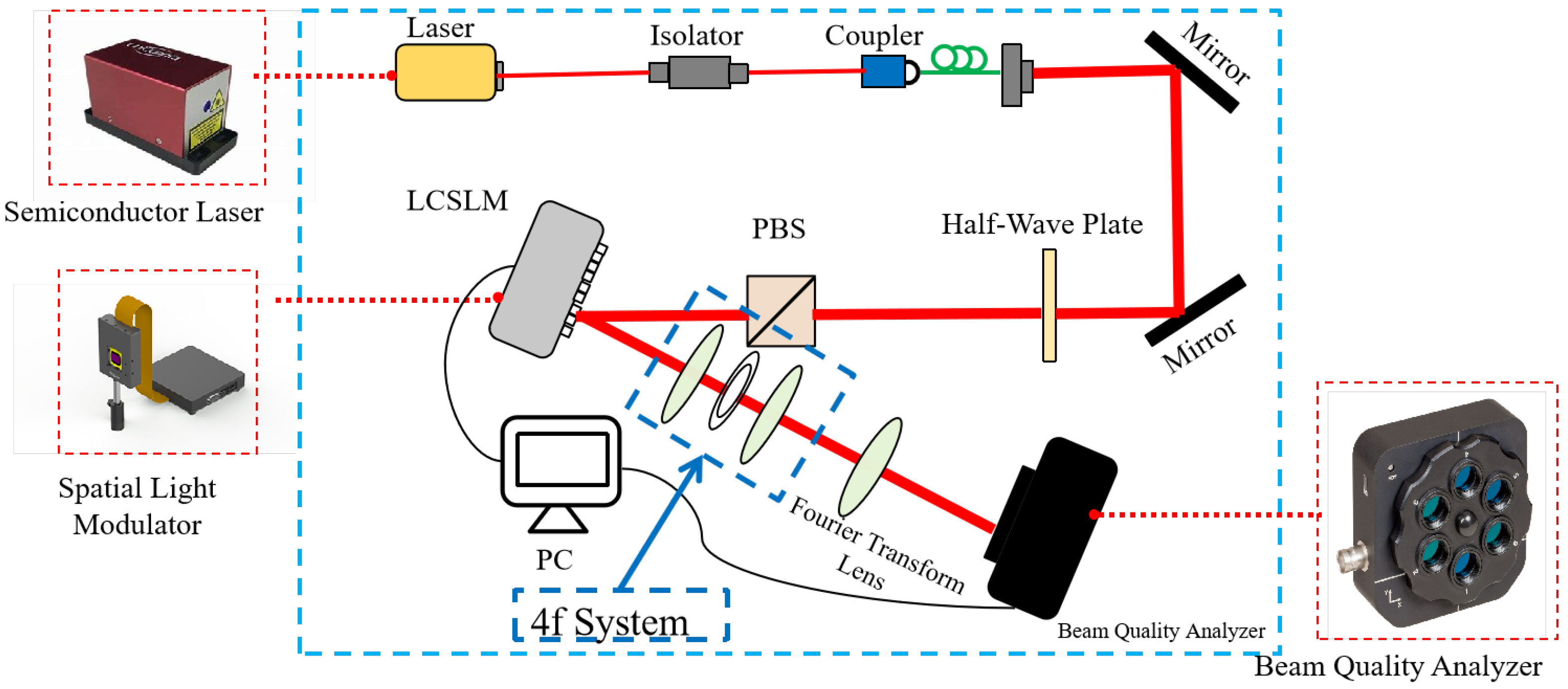
Given the reflective nature of the spatial light modulator (SLM) employed in this experiment, the fundamental optical path is designed as illustrated in Figure 2. The laser beam is first emitted from the laser diode, passes through an isolator, and is coupled into an optical fiber. After exiting the fiber, the beam undergoes expansion to achieve the desired spot size, followed by polarization via a polarizer to produce a horizontally linearly polarized beam. This beam then enters the SLM, where its phase is modulated. The reflected beam is focused by a convex lens and observed using a beam quality analyzer.

2.1. Phase Algorithms and Simulation

2.1.1. Gerchberg–Saxton (GS) Algorithm

The GS algorithm, proposed by Gerchberg and Saxton in 1971, remains a foundational approach in holographic computation and phase retrieval. It is based on iterative Fourier transforms and is known for its simplicity and ease of implementation. Figure 3 illustrates the algorithm’s workflow.
Let the incident beam have amplitude f 0 ( x 1 , y 1 ) and initial phase ϕ 0 ( x 1 , y 1 ) . After k iterative Fourier transforms, the output amplitude distribution is g o ( x k , y k ) , and the corresponding phase is ϕ k ( x k , y k ) . The initial optical field is E, and E k is expressed as the output optical field distribution. Substituting the initial phase into E yields the following:
E = f 0 x 1 , y 1 exp i ϕ 0 x 1 , y 1
A Fourier transform yields the following:
E 1 = F x 2 , y 2 exp i ϕ x 2 , y 2
Replacing the amplitude with the desired distribution:
E 1 = g 0 x 2 , y 2 exp i ϕ x 2 , y 2
Performing another Fourier transform yields the following:
E 1 = f x 1 , y 1 exp i ϕ x 2 , y 2
The updated field is obtained by replacing the amplitude with the original f ( x 1 , y 1 ) with the original f 0 ( x 1 , y 1 ) , maintaining the phase:
E 1 = f 0 x 1 , y 1 exp i ϕ x 2 , y 2
This iteration continues until the convergence condition (e.g., output phase ϕ k ( x k , y k ) ) is met.
In simulation, the following parameters are used: Gaussian and flat-top beam waist radius of 2 mm, resolution of 512 × 512 sampling points, SLM pixel size of 9.2 µm, focal length of Fourier lens of 100 mm, Super-Gaussian order of 10, and 50 iterations.
The simulation results are presented in Figure 4. The mean square error is 35.27%, and the top non-uniformity is 20.82%. The output beam demonstrates significant noise and suboptimal flatness.
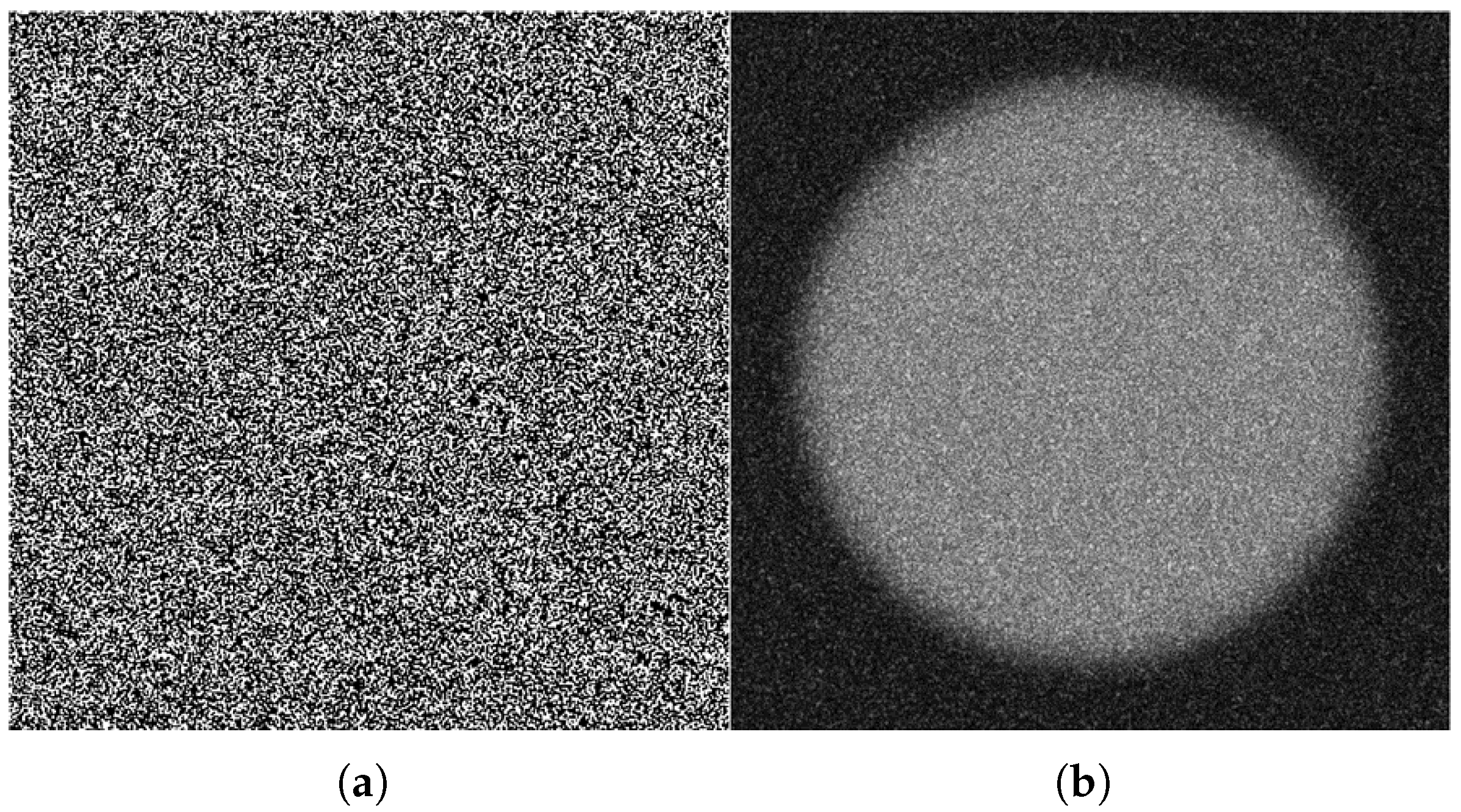
The phase distribution obtained by the GS algorithm is converted into a grayscale image as shown in Figure 5a, indicating significant disorder in the phase distribution. The grayscale values of adjacent pixels exhibit a jump-like distribution, making it difficult to reproduce such results in experiments. Figure 5b presents the simulation result of the beam shaping experiment using this phase distribution, which also shows severe noise and an unsatisfactory flat-top effect.
The GS algorithm is highly sensitive to the initial values of iterations during experiments, prone to falling into local optimal solutions, and stopping iterations, so the experimental effects are generally unsatisfactory. However, due to its simple principle, it provides an idea for people to study iterative algorithms, thus holding very important significance in iterative algorithms.

2.1.2. Improved Algorithm Based on GS and CNN

In recent years, with the advancement of neural network-related technologies, an increasing number of fields have begun to adopt this machine learning theory to explain complex experimental phenomena. Owing to its superior mapping and simulation capabilities, significant achievements have been made in various domains. For instance, in the research field of computer-generated holography (CGH), Hossein proposed an innovative non-iterative algorithm based on an unsupervised learning convolutional neural network called DeepCGH, aiming to enhance the quality of holograms through computation [37]. P. Tsang proposed a deep learning-based holographic vision system (HVS) that identifies holograms through hologram classification and uses a handwritten digit dataset for performance evaluation [38]. Goi presented a deep learning-based method for generating binary holograms, which generates binary holograms in a non-iterative manner and compares the neural network-generated binary holograms with those from existing methods, showing significant improvements in both speed and quality [39]. In 2010, researchers proposed a deep learning-based computer-generated holography (CGH) technique that can quickly generate high-quality holograms, outperforming baseline methods that require more computational resources and time [40]. S.J. Lee et al. proposed a deep learning-based digital holographic microscopy (DHM), where the network is trained on thousands of blurred microparticle holograms, uses a convolutional neural network (CNN) to estimate the depth of microparticles, and employs Segnet and Hough transform to detect microparticles in the plane. After training, this method far surpasses iterative methods in tracking the 3D motion of microparticles [41].
CNN (Convolutional Neural Network) possesses unique working principles and characteristics. Its local perception property enables neurons in the network to perceive only local regions of the input data, which is consistent with the local correlation characteristics of data such as images [42]. For instance, when processing light intensity images, adjacent pixels usually exhibit strong correlations, and local perception can effectively extract these local features [43]. Another core feature of CNN is the weight-sharing mechanism, which is manifested in the convolutional layer as follows: the weight parameters of the same convolution kernel remain consistent across the entire input data. This design significantly reduces the number of network parameters, effectively lowering the model complexity and the risk of overfitting [44]. The standard structure of CNN consists of convolutional layers, pooling layers, and fully connected layers. The convolutional layer performs feature extraction on input data through filters; the pooling layer reduces the dimensionality of feature maps while retaining key feature information (e.g., max pooling achieves feature compression by selecting the maximum value in local regions); the fully connected layer ultimately completes feature integration and classification decisions [45]. This hierarchical structure enables CNN to automatically learn feature representations with translation invariance [42]. CNN has demonstrated tremendous advantages in the field of image processing, being capable of automatically learning complex feature patterns in images. For example, in image classification tasks, it can accurately identify images of different categories, and it also exhibits excellent performance in tasks such as image denoising and super-resolution reconstruction [46,47].
Since the GS algorithm is a local optimization method, it is significantly influenced by the initial phase, making it prone to convergence at local optima. A well-designed initial solution can substantially enhance the performance of the GS algorithm. Therefore, the core idea of this study is to employ a CNN model to predict the initial phase distribution, followed by refinement using the GS algorithm.
The improved algorithm comprises four stages: data preparation, model training, phase prediction, and GS-based refinement, as illustrated in Figure 6 and described in detail as follows.
  • Data preparation
A high-quality dataset is essential for accurate neural network modeling. The following strategy is proposed:
Based on the equation E 2 x 2 , y 2 = F E 1 x 1 , y 1 × exp i ϕ 1 x 1 , y 1 , there E m ( m = 1 , 2 ) stands for light field distribution. Given E 1 , once a phase distribution Φ 1 is obtained, the corresponding intensity distribution E 2 can be computed. Thus, a set of random phase patterns Φ 1 is generated, and their corresponding intensity distributions E 2 ( x 2 , y 2 ) are obtained via simulation. The intensity E 2 serves as the input, and the phase Φ 1 as the ground-truth label output for training purposes to obtain the simulation of F ^ 1 by a neural network. A total of 500 data samples are synthesized and normalized to the grayscale range of [ 0 ,   1 ] .
  • Model Training
The CNN is implemented using the PyTorch1.10.2 framework. The network takes intensity distributions E 2 as input and padding was used to preserve the spatial dimensions, then learns to reconstruct the corresponding initial phase distributions Φ 1 . The Adam optimizer is employed, with a learning rate of 0.001 and 200 training epochs. The model minimizes the loss function, such as the Mean Squared Error (MSE), through backpropagation. During training, the validation set is periodically evaluated to monitor performance metrics such as phase correlation coefficients. Early stopping or regularization techniques may be applied if overfitting is detected.
  • Phase Prediction
Loading the Trained Model:After completing model training and confirming its satisfactory performance on the validation and test sets, load the trained model weights.
Inputting the Intensity Image to be Processed: Input the intensity images required for beam shaping in practical applications into the loaded model. These images must undergo the same pre-processing steps as the training data.
Outputting the Predicted Initial Phase: The model performs forward propagation calculations to output the corresponding initial phase distribution, which will serve as the initial input for the improved GS algorithm.
  • GS-Based Refinement
The predicted phase distribution φ ( X , Y ) is used to construct the initial complex amplitude for the GS algorithm. The algorithm then iteratively optimizes the phase to match the target intensity distribution. Convergence is defined by a predefined criterion—e.g., the error between the calculated and target intensity patterns remains below a threshold for consecutive iterations. Upon convergence, the resulting phase is considered optimal and can be used to drive spatial light modulators for beam shaping purposes.
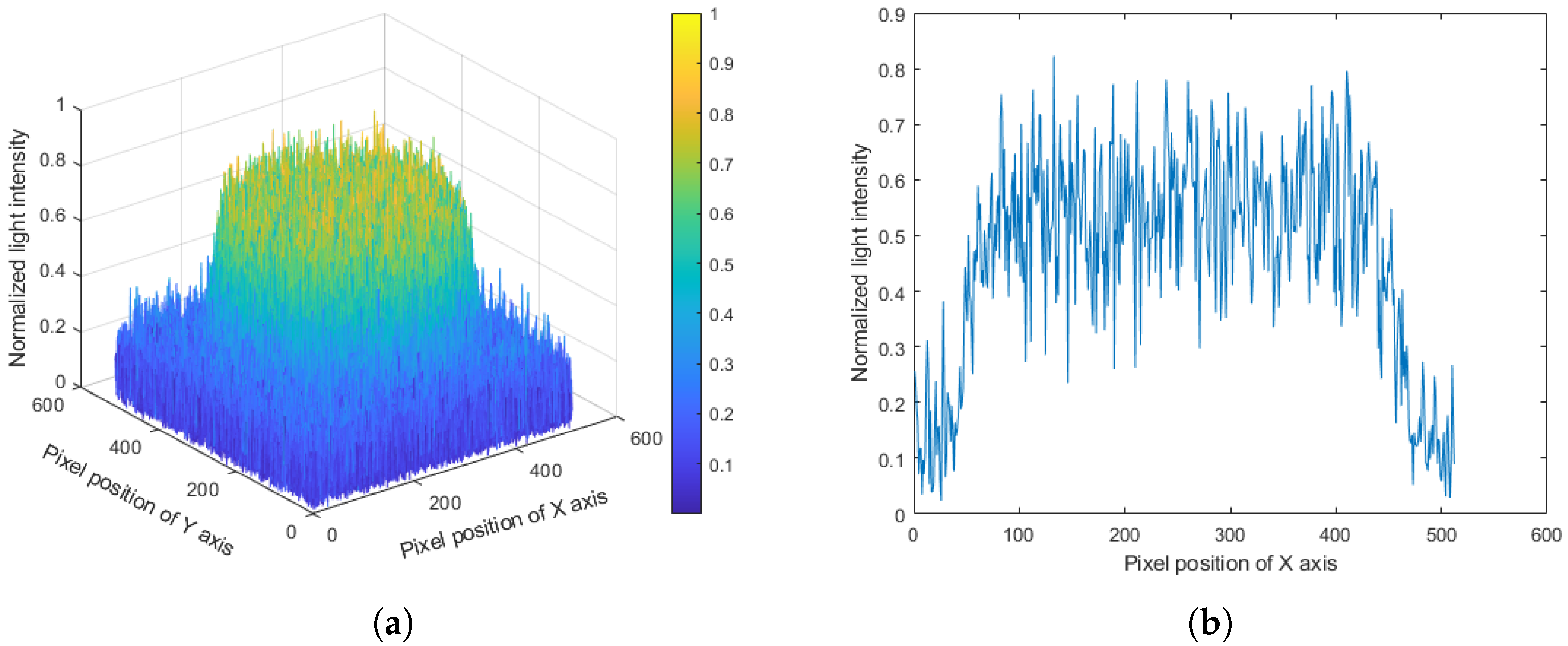
Figure 7 presents the simulation results of the improved GS algorithm assisted by the CNN model. Sub-figure (a) shows the 3D intensity profile of the generated flat-top beam, while (b) illustrates the cross-sectional intensity distribution. The Mean Squared Error (MSE) is 18.95%, and the peak non-uniformity is 7.56%. Compared to the GS algorithm, the improved method significantly enhances beam shaping quality.
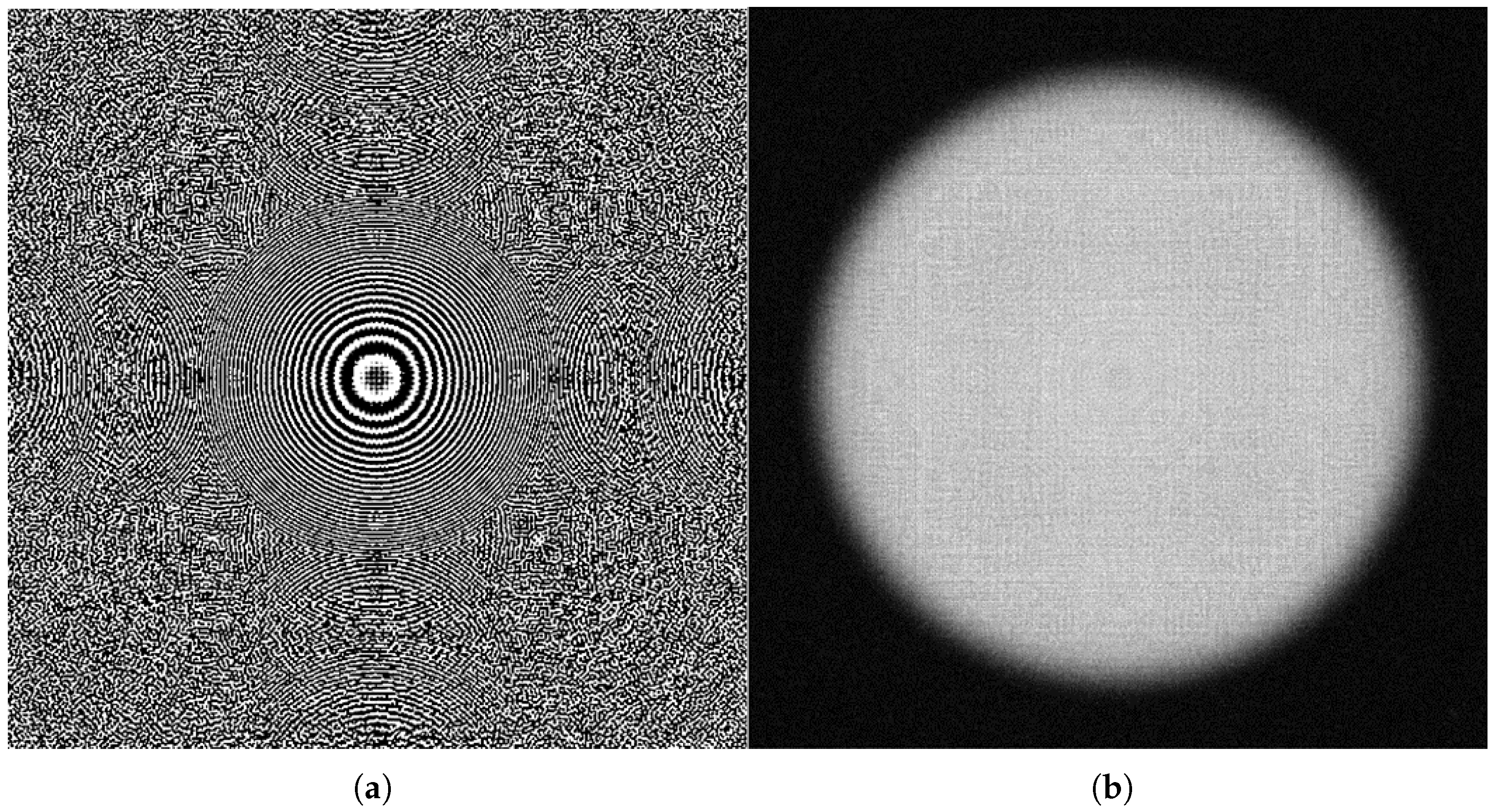
Figure 8 further evaluates the phase and beam quality. Sub-figure (a) shows the optimized phase hologram obtained by the improved method, characterized by smooth gray level transitions and reduced abrupt phase jumps. Sub-figure (b) displays the resulting two-dimensional flat-top beam intensity distribution, exhibiting superior uniformity compared to those produced by the GS.
Table 1 summarizes the comparative results among the algorithms above. The proposed method achieves the lowest MSE and peak non-uniformity, demonstrating its superior performance in beam shaping tasks.

3. Training and Experiments

3.1. Dataset Preparation

Due to the absence of publicly available datasets suitable for training deep neural networks in computer-generated holography, a custom dataset was generated.
According to the equation E 2 ( x 2 , y 2 ) = F [ E 1 ( x 1 , y 1 ) × exp ( i Φ 1 ( x 1 , y 1 ) ) ] , a known input amplitude E 1 and a Φ 1 can generate a corresponding E 2 , so a series of phase distributions Φ 1 can be randomly generated, the output field intensity E 2 ( x 2 , y 2 ) can be computed and saved then. This enables the creation of input-output pairs: E 2 as input, Φ 1 as output, to train a supervised learning model to obtain the simulation of F ^ 1 .
In this simulation, 500 sets of 64 × 64 data were generated and normalized to grayscale values in the range [ 0 ,   1 ] . Data were saved in . n p y format for training and also exported as . p n g images for visualization. Each sample was labeled by index; let s a m p l e _ n u m _ p h a s e and s a m p l e _ n u m _ a m p l i t u d e denote the phase distribution and its corresponding amplitude distribution, respectively. The phase and amplitude are numbered to establish their correspondence.

3.2. Network Architecture and Model Training

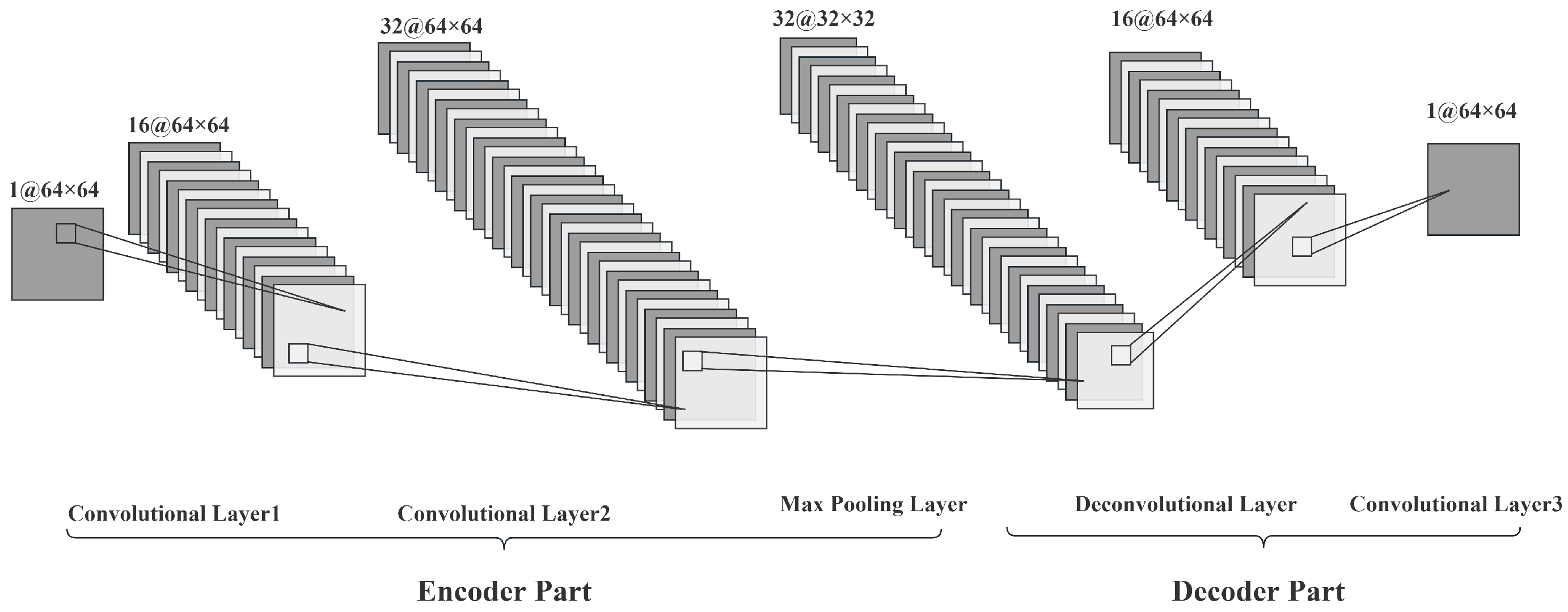
The model adopts an encoder–decoder structure similar to U-Net [48] that shows in Figure 9. In this paper, the model we used has a structure as follows: the encoder consists of two 3 × 3 convolutional layers that increase the channel dimension, followed by a max pooling layer to reduce spatial resolution. The decoder includes a transposed convolution layer to restore resolution and a final convolution layer to produce a 64 × 64 phase map. A ReLU activation function follows each layer to maintain nonlinearity for the advantage of enabling efficient training of deep networks through simple piecewise nonlinearity, while avoiding the vanishing gradient and computational redundancy issues of sigmoid. In contrast, the strong and smooth nonlinearity of the sigmoid has only limited applications in shallow networks or specific output layers, and it has been replaced by ReLU and its variants (such as Leaky ReLU and Swish) in hidden layers. After the ReLU activation function, a Dropout layer with a dropout rate of 0.5 and L2 regularization was added.
The training procedure includes the following steps:
  • Set parameters: path for datasets saving, input image size 64 × 64, batchsize 8, learning rate 1 × 10⁻³, training epochs 200, and loss function as RMSE.
  • Initialize model weights.
  • For each epoch, input training data to perform forward propagation, compute output, and calculate loss against the ground-truth phase. To enhance the credibility of the trained model, in the absence of a separate validation set, we employed 5-fold cross-validation on the 500 generated samples during training. Specifically, the dataset was randomly partitioned into 5 subsets of equal size (100 samples each). In each fold, 4 subsets (400 samples) served as the training data, and the remaining 1 subset (100 samples) was used to monitor performance metrics such as phase correlation coefficients for hyperparameter tuning. This process was repeated 5 times, with each subset acting as the validation data exactly once. The average performance across all folds was taken to guide hyperparameter selection, ensuring that the model optimization was based solely on the training data distribution. Meanwhile, a separate test set, consisting of 100 additional samples generated using the same method but not involved in any training or cross-validation steps, was reserved to provide an unbiased final evaluation of the model’s generalization ability.
  • Perform backpropagation to compute gradients.
  • Update weights using the Adam optimizer in view of its advantage lies in its balance between convergence speed, stability, and parameter adaptability, with low dependence on hyperparameters, enabling it to quickly achieve favorable results in most deep learning tasks. Although in certain scenarios (such as image classification requiring extreme generalization performance), Stochastic Gradient Descent (SGD) combined with fine hyperparameter tuning may perform slightly better, Adam has become the default choice in both industry and academia due to its comprehensive performance.
  • Repeat until convergence or max epochs reached.
  • Save model weights upon training completion.
Detailed parameter settings in Table 2.
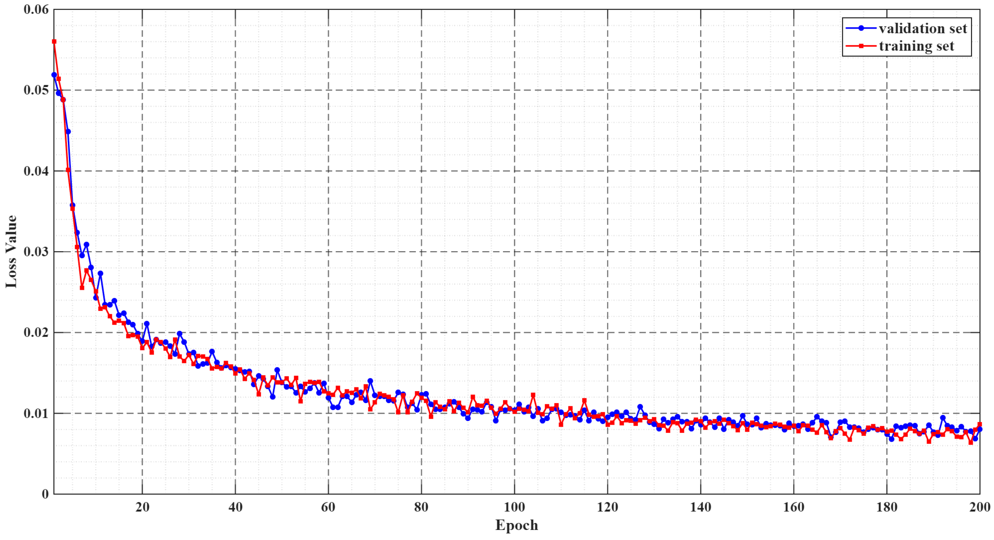
Figure 10 shows the loss function curves of the training set and validation set of the proposed algorithm after 200 training epochs. The curve trends indicate the following: In the early training stage (0–25 epochs), the loss values of both sets decrease rapidly, demonstrating effective adjustment of network parameters. In the middle training stage (25–170 epochs), the loss values show a fluctuating slow decline, indicating that the network is undergoing fine–tuning. In the final training stage (170–200 epochs), the loss values tend to be stable and finally converge to around 0.01, proving that the network has reached a good convergence state. The blue curve represents the validation set, and the red curve represents the training set, enabling a direct comparison of their loss change trends during the training process. The shared y-axis enhances the clarity of comparing the magnitude and rate of loss reduction between the two curves, providing a more intuitive understanding of the model’s generalization ability during training.
Model inference steps are as follows: (1) Load trained model and weights. (2) Resize the target amplitude image to match the model input. (3) Feed into the network to obtain the predicted initial phase. (4) Input the phase into the GS algorithm for refinement. (5) Save the final phase hologram and load it onto the SLM for physical beam shaping.

3.3. Optical Setup

To reduce optical noise introduced by the LCSLM, a 4 f filtering system is implemented. As shown in Figure 11, a pair of identical focal length lenses is placed after the LCSLM with a separation of 2 f . A spatial filter (aperture) at the Fourier plane blocks the zero-order diffraction component. An imaging lens is placed at one focal length after the 4 f system.
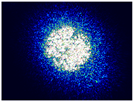
The effectiveness of the 4 f system is summarized in Table 3. Without filtering, shaped beams contain high noise and large non-uniformity. Introducing the 4 f system improves beam uniformity significantly.

3.4. Experimental Procedure

The experimental procedure for phase-modulated beam shaping is described as follows:
First, the optical setup is constructed. According to the optical path layout shown in Figure 11, all components are properly positioned, and the laser beam height and collimation are finely adjusted. The laser source emits a beam at a wavelength of 795 nm, with an initial Gaussian intensity profile. A beam expansion system composed of two convex lenses with focal lengths of 25 mm and 75 mm is used to enlarge the beam spot by a factor of three. The beam then passes through a half-wave plate and a polarizing beam splitter (PBS) to adjust the polarization state to horizontal linear polarization. After incidence on the liquid crystal spatial light modulator (SLM), the corresponding phase map is loaded onto the SLM. The reflected beam is then passed through a 4 f filtering system and a Fourier lens, with a beam quality analyzer positioned at the back focal plane of the Fourier lens to observe the beam shaping results.
Second, the phase map calculation is conducted. A critical aspect of this experiment is the accurate computation of the phase distribution to be loaded onto the SLM. The required experimental parameters are input into the algorithm described in Section 2.1, for example: laser wavelength: 795 nm, flat-top beam waist radius: 80 mm, holographic phase map size: [ 1000 × 1000 ] , pixel size: 9.2 µm, Fourier lens focal length:100 mm. The algorithm is executed, and the resulting phase map [ π ,   π ] is saved as a grayscale image [ 0 ,   255 ] representing the target phase distribution over the designated region.
Finally, the grayscale phase map is uploaded to the SLM. Under the influence of the constructed optical system, the laser beam acquires the fixed phase modulation imparted by the SLM. After propagation through the Fourier lens, the intensity distribution of the beam is transformed into a flat-top profile with uniform intensity within a defined area. The resulting beam shape can be directly observed using the beam quality analyzer.

4. Results and Discussion

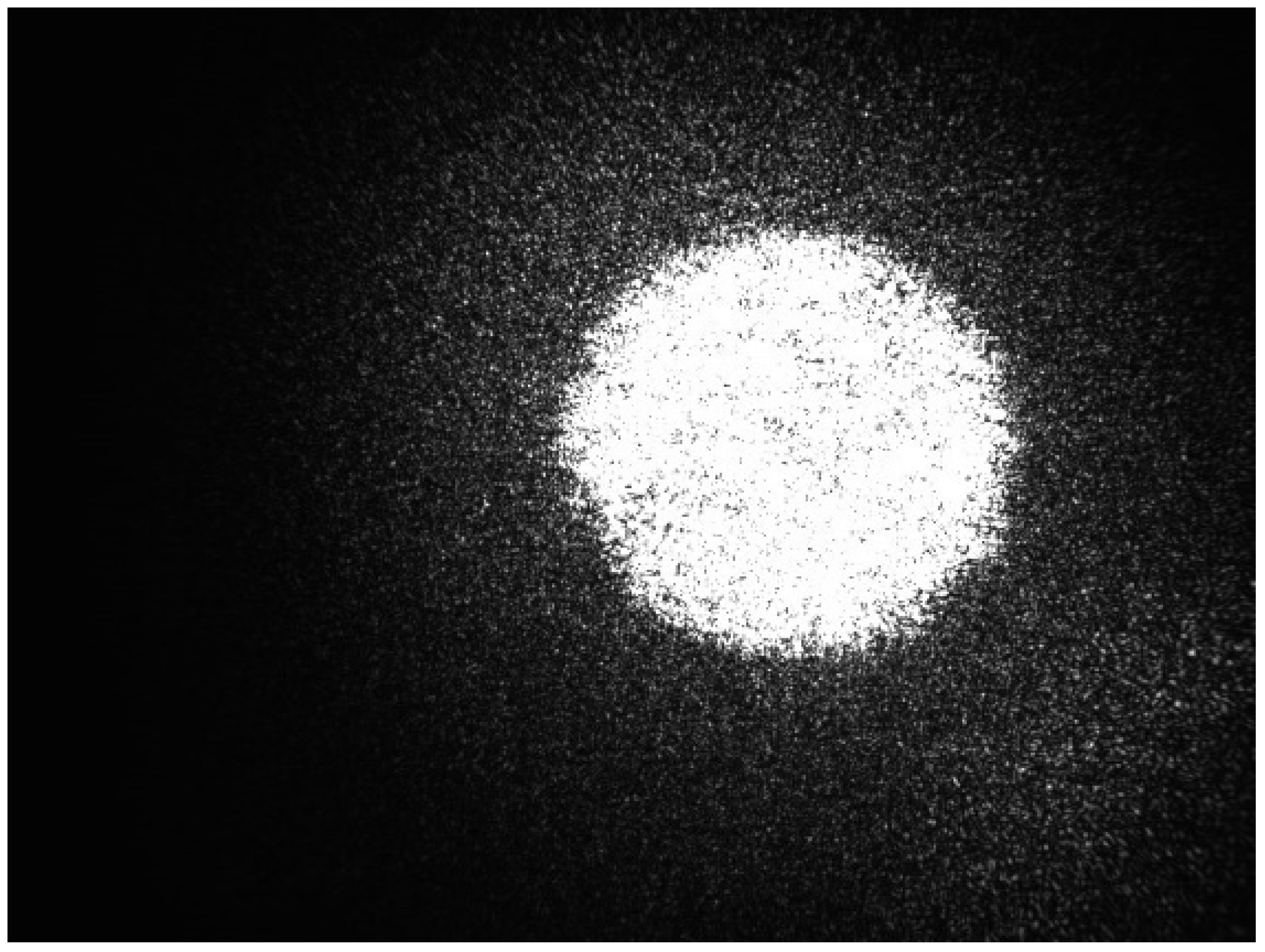
The phase hologram calculated by the proposed algorithm was uploaded to the liquid crystal spatial light modulator (LCSLM). By spatially separating the zero-order diffraction spot from the modulated beam, a circular flat-top beam was successfully generated, as shown in Figure 12.
To quantitatively evaluate beam shaping performance, the experimental data were imported into MATLAB R2024b for analysis. The cross-sectional intensity distribution along the x-axis of the circular flat-top beam is shown in Figure 13.
From the experimental data, the flat-top region is observed to lie within the interval [ 360 ,   610 ] . By extracting this segment and applying Equation (5), the peak non-uniformity was calculated to be 5.07%, consistent with theoretical expectations.
This study introduces an innovative enhancement to the classical Gerchberg–Saxton (GS) phase retrieval algorithm by incorporating an optimized computational model to obtain the phase solution. Numerical simulations showed a reduction in the peak non-uniformity of the output beam to 7.56%. A complete optical experimental system was then established based on the simulation framework, producing a circular flat-top beam with a measured peak non-uniformity of 5.07%. The experimental results exhibit strong agreement with simulation predictions. An error source analysis of the system indicates that discrepancies mainly arise from the following three aspects: ( 1 ) Deviation between ideal and actual input beam profiles: The numerical model assumes an ideal Gaussian beam, whereas the experimentally generated beam exhibits non-ideal features. This asymmetry in input conditions significantly limits the achievable uniformity of the output beam. ( 2 ) Phase quantization error of the LCSLM: The 8−bit (256−level) discrete grayscale modulation introduces quantization errors in phase representation. Additionally, the approximate linear relationship between grayscale and phase is only maintained within a limited range, resulting in phase reconstruction inaccuracies during phase mask generation. ( 3 ) Geometric misalignments in optical alignment: (a) The laser beam center and the geometric center of the LCSLM’s modulation area are difficult to align precisely. (b) Diffraction effects from the edges of the aperture in the spatial filtering stage impose additional wavefront modulation on the output beam.

5. Conclusions

In conclusion, this study experimentally verifies the effectiveness of the proposed beam shaping method in enhancing the sensitivity of SERF atomic magnetometers with the Rb (rubidium) cell, and the experimental schematic and partial physical setup of a SERF atomic magnetometer are shown in Figure 14. The research demonstrates that modifying the Gaussian laser pump via a CNN-GS hybrid algorithm leads to significant performance improvements in ultra-sensitive magnetic field measurement devices based on atomic spin effects. The comparison results of sensitivity values between the method in this paper and traditional methods are shown in Figure 15. Specifically, when using the default Gaussian laser as the pump without phase modulation, the atomic magnetometer exhibited a sensitivity of 14.04 fT/Hz1/2. Upon introducing the CNN-GS hybrid algorithm we proposed, the sensitivity was improved to 7.80 fT/Hz1/2, representing a 44% enhancement. This result is in good agreement with theoretical predictions. Furthermore, the algorithm proposed not only boosts sensitivity but also improves laser quality, mitigating potential damage to optical components and devices. These findings highlight the method’s dual utility in optimizing measurement precision and extending device longevity.

Author Contributions

Conceptualization, Y.L. and F.L.; methodology, F.L.; software, M.S.; validation, M.S. and F.L.; formal analysis, M.S.; investigation, Q.C. and Y.Z.; resources, Q.C. and Y.Z.; data curation, M.S. and F.L.; writing—original draft preparation, M.S. and F.L.; writing—review and editing, Y.L. and M.S.; visualization, M.S.; supervision, Y.L. and Y.Z.; project administration, Y.L.; funding acquisition, Y.Z. All authors have read and agreed to the published version of the manuscript.

Funding

This work was supported in part by the National Key Research and Development (R&D) Plan under Grant 2024YFB3212500; in part by the Innovation Program for Quantum Science and Technology under Grant 2021ZD0300503.

Data Availability Statement

Data underlying the results presented in this paper are not publicly available at this time but may be obtained from the authors upon reasonable request.

Conflicts of Interest

The authors declare that there are no conflicts of interest related to this article.

References

  1. Wei, K.; Xu, Z.; He, Y.; Ma, X.; Heng, X.; Huang, X.; Quan, W.; Ji, W.; Liu, J.; Wang, X.-P. Dmitry Budker and Jiancheng Fang Dark matter search with a resonantly-coupled hybrid spin system. Rep. Prog. Phys. 2025, 88, 057801. [Google Scholar] [CrossRef]
  2. Dang, H.B.; Maloof, A.C.; Romalis, M.V. Ultra-high sensitivity magnetic field and magnetization measurements with an atomic magnetometer. Appl. Phys. Lett. 2010, 97, 151110. [Google Scholar] [CrossRef]
  3. Kominis, I.K.; Kornack, T.W.; Allred, J.C.; Romalis, M.V. Dark matter search with a resonantly-coupled hybrid spin system. Nature 2003, 422, 596–599. [Google Scholar] [CrossRef]
  4. Tian, X.; Bao, B.; Wang, R.; Li, D. An FSM-assisted high-accuracy autonomous magnetic compensation optimization method for dual-channel SERF magnetometers used in weak biomagnetic signal measurement. Sensors 2025, 25, 3690. [Google Scholar] [CrossRef] [PubMed]
  5. Zhai, Y.; Yue, Z.; Li, L.; Liu, Y. Progress and applications of quantum precision measurement based on SERF effect. Front. Phys. 2022, 10, 969129. [Google Scholar] [CrossRef]
  6. Shah, V.; Romalis, M.V. Spin-exchange relaxation-free magnetometry using elliptically polarized light. Phys. Rev. A 2009, 80, 013416. [Google Scholar] [CrossRef]
  7. Yan, Y.; Zhang, S.; Liu, Z.; Zhan, D.; Liu, Z.; Li, X.; Zhou, Y.; Lu, J. Optical parameter decoupling and optimization for an elliptically polarized atomic magnetometer. IEEE Trans. Instrum. Meas. 2024, 73, 1500210. [Google Scholar] [CrossRef]
  8. Liu, Y.; Huang, B.; Li, J.; Li, R.; Zhai, Y. Flow rate estimation based on magnetic particle detection using a miniaturised high-sensitivity OPM. IEEE Trans. Instrum. Meas. 2025, 74, 9518010. [Google Scholar] [CrossRef]
  9. Zou, S.; Jin, G.; Shi, T.; Zhang, H. Determination of mole fractions in alkali-metal mixtures via collisional broadening from Van der Waals interactions. Measurement 2025, 244, 116544. [Google Scholar] [CrossRef]
  10. Allred, J.C.; Lyman, R.N.; Kornack, T.W.; Romalis, M.V. High-sensitivity atomic magnetometer unaffected by spin-exchange relaxation. Phys. Rev. Lett. 2002, 89, 130801. [Google Scholar] [CrossRef]
  11. Wakai, R.T. The atomic magnetometer: A new era in biomagnetism. In Proceedings of the AIP Conference, Baltimore, ML, USA, 15–18 April 2014; pp. 133–136. [Google Scholar]
  12. Xia, H.; Ben-Amar Baranga, A.; Hoffman, D.; Romalis, M.V. Magnetoencephalography with an atomic magnetometer. Appl. Phys. Lett. 2006, 89, 211104. [Google Scholar] [CrossRef]
  13. Wyllie, R.; Kauer, M.; Smetana, G.S.; Wakai, R.T.; Walker, T.G. Magnetocardiography with a modular spin-exchange relaxation-free atomic magnetometer array. Phys. Med. Biol. 2012, 57, 2619. [Google Scholar] [CrossRef]
  14. DeLand, Z.J. Advances in Fetal Magnetocardiography Using SERF Atomic Magnetometers. Ph.D. Thesis, The University of Wisconsin-Madison, Madison, WI, USA, 2017. [Google Scholar]
  15. Sulai, I.A.; DeLand, Z.J.; Bulatowicz, M.D.; Wahl, C.P.; Wakai, R.T.; Walker, T.G. Characterizing atomic magnetic gradiometers for fetal magnetocardiography. Rev. Sci. Instrum. 2019, 90, 085003. [Google Scholar] [CrossRef]
  16. Li, X.; Han, B.; Zhang, K.; Liu, Z.; Wang, S.; Yan, Y.; Lu, J. All-optical dual-axis zero-field atomic magnetometer using light-shift modulation. Phys. Rev. Appl. 2024, 21, 014023. [Google Scholar] [CrossRef]
  17. Zhang, Y.; Tang, J.; Xu, X.; Wang, Z.; Zhai, Y. Design and analysis of a high-sensitivity atomic magnetic gradiometer with adjustable baseline. IEEE Trans. Instrum. Meas. 2025, 74, 1501109. [Google Scholar] [CrossRef]
  18. Tang, J.; Liu, Y.; Wang, Y.; Zhou, B.; Han, B.; Zhai, Y.; Liu, G. Enhancement of bandwidth in spin-exchange relaxation-free (SERF) magnetometers with amplitude-modulated light. Appl. Phys. Lett. 2022, 120, 084001. [Google Scholar] [CrossRef]
  19. Bell, W.E.; Bloom, A.L. Optical detection of magnetic resonance in alkali metal vapor. Phys. Rev. 1957, 107, 1559–1565. [Google Scholar] [CrossRef]
  20. Li, R.; Liu, Y.; Cao, L.; Li, S.; Li, J.; Zhai, Y. Parameter optimisation of miniaturised SERF magnetometer below relaxation rate saturation region. Measurement 2023, 214, 112733. [Google Scholar] [CrossRef]
  21. Li, Z.M.; Wakai, R.T.; Walker, T.G. Research on Optical Frequency Shift Suppression and Beam Uniformity. Chin. J. Lasers 2024, 51, 0312001. [Google Scholar]
  22. Asphericon. Aspheric Beam Shapers [EB/OL]. Available online: https://www.asphericon.com/en/products/beamtuning/beamshaping (accessed on 25 June 2025).
  23. Mao, J.Y.; Wang, M.; Wang, Q.T.; Liu, L.R. Laser beam shaping system with a radial birefringent filter. J. Mod. Opt. 2006, 54, 129–136. [Google Scholar]
  24. Kornack, T.W.; Allred, J.C.; Romalis, M.V. Subfemtotesla atomic magnetometer. Appl. Phys. Lett. 2003, 82, 3498–3500. [Google Scholar]
  25. Li, Z.M.; Wakai, R.T.; Walker, T.G. Parametric modulation of an atomic magnetometer. Appl. Phys. Lett. 2006, 89, 134105. [Google Scholar] [CrossRef] [PubMed]
  26. Hamamatsu Photonics. Liquid Crystal on Silicon Spatial Light Modulators (LCoS-SLM) [EB/OL]. Available online: https://lcos-slm.hamamatsu.com/jp/en/learn/about_lcos-slm/comparison.html (accessed on 25 June 2025).
  27. Gerchberg, R.W.; Saxton, W.O. A practical algorithm for the determination of phase from image and diffraction plane pictures. Optik 1972, 35, 237–246. [Google Scholar]
  28. Zhang, Y.; Sun, M. Simulated annealing applied to HIO method for phase retrieval. Photonics 2021, 8, 541. [Google Scholar] [CrossRef]
  29. Taylor, J.R. Phase Retrieval Using a Genetic Algorithm on the Systematic Image-Based Optical Alignment Test Bed; NASA/CR-2003-212397; National Aeronautics and Space Administration (NASA): Washington, DC, USA, 2003. [Google Scholar]
  30. Fienup, J.R. Phase retrieval algorithms: A comparison. Appl. Opt. 1982, 21, 2758–2769. [Google Scholar] [CrossRef]
  31. Eglese, R.W. Simulated annealing: A tool for operational research. Eur. J. Oper. Res. 1990, 46, 271–281. [Google Scholar] [CrossRef]
  32. Ma, W.; Liu, Z.C.; Kudyshev, Z.A.; Boltasseva, A.; Cai, W.S.; Liu, Y.M. Deep learning for the design of photonic structures. Nat. Photonics 2021, 15, 77–90. [Google Scholar] [CrossRef]
  33. Dawson, R.; O’Dwyer, C.; Irwin, E.; Mrozowski, M.S.; Hunter, D.; Ingleby, S.; Riis, E. Automated Machine Learning Strategies for Multi-Parameter Optimisation of a Caesium-Based Portable Zero-Field Magnetometer. Sensors 2023, 23, 4007. [Google Scholar] [CrossRef]
  34. Liu, J.; Yuan, Y.; Pei, H.; Lei, X.; Xia, H.; Wang, W. LSA-PINN: A New Method Based on Physics-Informed Neural Network with Lightweight Self-Attention for Solving Modified Bloch Equation. Results Phys. 2024, 61, 107716. [Google Scholar] [CrossRef]
  35. Babaei, B.; Smith, B.D.; Tretiakov, A.; Narayanan, A.; LeBlanc, L.J. Microwave-Optical Double-Resonance Vector Magnetometry with Warm Rb Atoms. arXiv 2025, arXiv:2507.08791. [Google Scholar]
  36. Lam, H.S.; Tsang, P.W.M. Invariant classification of holograms of deformable objects based on deep learning. In Proceedings of the 2019 IEEE 28th International Symposium on Industrial Electronics (ISIE), Vancouver, BC, Canada, 12–14 June 2019; IEEE: New York, NY, USA, 2019; pp. 2392–2396. [Google Scholar]
  37. Eybposh, H.; Caira, N.W.; Atisa, M.; Chakravarthula, P. DeepCGH: 3D computer-generated holography using deep learning. PLoS Comput. Biol. 2020, 16, e1008293. [Google Scholar]
  38. Tsang, P.W.M.; Lam, H. Holographic vision system based on non-diffractive optical scanning holography and deep learning. In Proceedings of the Holography, Diffractive Optics, and Applications IX, Hangzhou, China, 21–23 October 2019; SPIE: Bellingham, WA, USA, 2019; Volume 11188, pp. 61–66. [Google Scholar]
  39. Goi, H.; Komuro, K.; Nomura, T. Deep-learning-based binary hologram. Appl. Opt. 2020, 59, 7103–7108. [Google Scholar] [CrossRef]
  40. Eybposh, M.H.; Caira, N.W.; Chakravarthula, P.; Atisa, M.; Pégard, N.C. High-speed computer-generated holography using convolutional neural networks. In Proceedings of the Optics and the Brain, Virtual, 20–23 April 2020; Optica Publishing Group: Washington, DC, USA, 2020. [Google Scholar]
  41. Lee, S.J.; Yoon, G.Y.; Go, T. Deep learning-based accurate and rapid tracking of 3D positional information of microparticles using digital holographic microscopy. Exp. Fluids 2019, 60, 170. [Google Scholar] [CrossRef]
  42. LeCun, Y.; Bottou, L.; Bengio, Y.; Haffner, P. Gradient-based learning applied to document recognition. Proc. IEEE 1998, 86, 2278–2324. [Google Scholar] [CrossRef]
  43. Shen, W.; Wu, X.; Zhang, D. Deep learning for optical metrology: A review. Opt. Lasers Eng. 2017, 98, 27–40. [Google Scholar]
  44. Krizhevsky, A.; Sutskever, I.; Hinton, G.E. ImageNet classification with deep convolutional neural networks. In Proceedings of the Advances in Neural Information Processing Systems 25 (NIPS 2012), Lake Tahoe, NV, USA, 3–8 December 2012; pp. 1097–1105. [Google Scholar]
  45. Simonyan, K.; Zisserman, A. Very deep convolutional networks for large-scale image recognition [EB/OL]. arXiv 2014, arXiv:1409.1556. [Google Scholar]
  46. Dong, C.; Loy, C.C.; He, K.; Tang, X. Image super-resolution using deep convolutional networks. IEEE Trans. Pattern Anal. Mach. Intell. 2016, 38, 295–307. [Google Scholar] [CrossRef]
  47. Chen, Y.; Wang, L. Speckle noise reduction in optical coherence tomography images using convolutional neural networks. Opt. Lett. 2018, 43, 2651–2654. [Google Scholar]
  48. Ronneberger, O.; Fischer, P.; Brox, T. U-net: Convolutional networks for biomedical image segmentation. In Proceedings of the Medical Image Computing and Computer-Assisted Intervention–MICCAI 2015: 18th International Conference, Munich, Germany, 5–9 October 2015; Proceedings, Part III 18. Springer International Publishing: Berlin/Heidelberg, Germany, 2015; pp. 234–241. [Google Scholar]
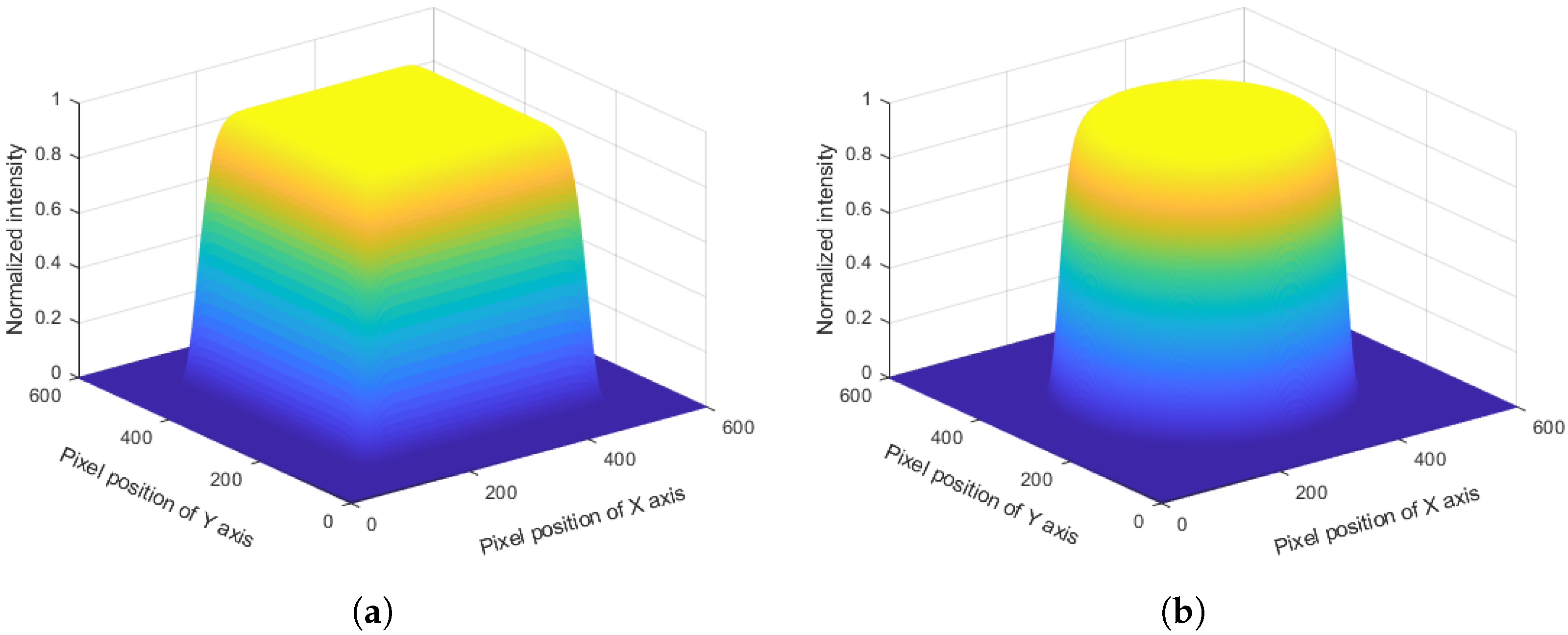
Figure 1. Three-dimensional intensity distributions of circular and square flat-top beams: (a) 3D intensity distribution of a circular flat-top beam. (b) 3D intensity distribution of a square flat-top beam.
Photonics 12 00796 g001
Figure 2. The basic optical path design of the atomic magnetic force pump light field based on phase modulation is generated.
Photonics 12 00796 g002
Figure 3. Flowchart of the Gerchberg–Saxton algorithm.
Photonics 12 00796 g003
Figure 4. Simulation results using the GS algorithm: (a) 3D intensity distribution of the GS-shaped circular flat-top beam. (b) Cross-sectional intensity profile.
Photonics 12 00796 g004
Figure 5. GS algorithm-generated phase and simulation output: (a) Phase hologram generated by GS algorithm. (b) 2D simulation of circular flat-top.
Photonics 12 00796 g005
Figure 6. Overall workflow of the improved algorithm.
Photonics 12 00796 g006
Figure 7. Simulation of the improved GS algorithm: (a) 3D intensity profile of the shaped flat-top beam. (b) Cross-sectional intensity distribution of the flat-top beam.
Photonics 12 00796 g007
Figure 8. Simulation Results of Improved Algorithm-Phase Hologram and Circular Flat-Top Beam Shaping: (a) Phase hologram obtained via the improved algorithm. (b) Simulated 2D flat-top beam distribution using the optimized phase.
Photonics 12 00796 g008
Figure 9. Schematic of the neural network architecture.
Photonics 12 00796 g009
Figure 10. Variation of error values with the number of training epochs on the training set and validation set.
Photonics 12 00796 g010
Figure 11. Modified optical system incorporating 4 f spatial filtering.
Photonics 12 00796 g011
Figure 12. Two-dimensional intensity distribution of the circular flat-top beam generated using the improved algorithm.
Photonics 12 00796 g012
Figure 13. X-axis intensity profile of the circular flat-top beam obtained from MATLAB analysis.
Photonics 12 00796 g013
Figure 14. (a) Experimental setup diagram of the single-beam SERF magnetometer. λ / 2 : λ / 2 wave plate. PBS: polarization beam splitter. λ / 4 : λ / 4 wave plate. BS: beam splitter. PD: photodetector. WG: waveform generator (Tektronix, AFG31000 SERIES). PID: Proportional Integration Differentiation. TIA: transimpedance amplifier (Thorlabs, PDA200C). LIA: lock-in amplifier(Zurich Instrument, HF2LI). DAQ: data acquisition. PC: personal computer. (bd) Photographs of some experimental system components. Oscilloscope: (RIGOL, DS7034). Wave Filter + Adder: (Stanford Research Systems, SIM Series).
Photonics 12 00796 g014aPhotonics 12 00796 g014b
Figure 15. Comparison of sensitivity curves obtained by pumping with Gaussian beams and flat-top beams.
Photonics 12 00796 g015
Table 1. Comparison of Simulation Results among GS and CNN-GS Hybrid Algorithms.
AlgorithmMean Squared Error (%)Peak Non-Uniformity (%)
GS Algorithm35.2720.82
Proposed CNN-GS Hybrid18.957.56
Table 2. Model training main parameter table.
ParametersSetting
convolutional Layer3 × 3
max pooling layer2 × 2
training epoch200
batchsize8
learning rate0.001
optimization algorithmAdam
loss functionMSE
activation functionReLU
regularizationDropout (0.5) + L2
Table 3. Comparison Before and After 4 f System.
BeforeAfter
Circular Flat-top beamPhotonics 12 00796 i001Photonics 12 00796 i002
Square Flat-top beamPhotonics 12 00796 i003Photonics 12 00796 i004
Disclaimer/Publisher’s Note: The statements, opinions and data contained in all publications are solely those of the individual author(s) and contributor(s) and not of MDPI and/or the editor(s). MDPI and/or the editor(s) disclaim responsibility for any injury to people or property resulting from any ideas, methods, instructions or products referred to in the content.