Subtraction Method for Subpixel Stitching: Synthetic Aperture Holographic Imaging

Abstract

Image stitching is a crucial technique in various fields of imaging and photography, which allows for the creation of high-resolution images by combining multiple smaller images with overlapping regions. Here, we propose a simple and fast method, the Subtraction Method (SM), for pixel and subpixel image stitching using holographic data. The feasibility of the SM is verified at the pixel and subpixel level using two 2D images captured by a 4-f imaging system. Additionally, the application of the SM for holographic data is also explored. The effective aperture of an inline holographic imaging system is enlarged by stitching four in-line holograms, demonstrating enhanced resolution and image quality after reconstruction. The stitching accuracy and computational time of the SM is compared with the correlation method. With optimization, the result shows that the SM achieves high accuracy and requires less computational time for image stitching when compared to contemporary image stitching algorithms.

1. Introduction

The image stitching or registration is the process of combining multiple images with overlapping areas to produce a seamless higher-resolution image [1,2]. Techniques based on image intensity (grey level), e.g., Sum of Absolute Value (SAD), and methods based on distinct feature extraction [3,4], are two general approaches to perform stitching. Image stitching has important applications in computer vision and biomedical image processing [3,4].

Image stitching involves three main process components: calibration, image registration, and blending [5,6]. The core process, registration, refers to the alignment of two or more images captured from different perspectives. The objective is to increase the effective system aperture, resulting in super-resolution image reconstruction.

When combining a series of displaced images, image stitching requires accurate estimation of the shifts between them. The higher the precision in aligning the images, with which the different images are combined, the greater the potential quality of the resulting image, i.e., its information content. Subpixel image registration is essential to achieve such accurate image alignment. The most commonly used method to determine displacement is the correlation method (CM) [7]. However, the CM is numerically intensive and suffers from bias errors [8]. Subpixel displacement is determined using the CM by either upsampling the digital images and/or interpolating the correlation function. Either approach significantly increases computational complexity.

Holography was discovered in 1948 by Denis Gabor, who proposed to use this technique to improve the resolution in electron microscopy, by reconstructing the total diffracted wavefront of an object, amplitude, and phase [9]. For his work Gabor was awarded the Nobel Prize 50 years ago in 1971. Digital holography (DH) refers to the acquisition and processing of holograms using a digital sensor. It has been applied in the fields of 3D imaging and display, deep learning, neural networks, microscopy, and metrology [9,10,11]. To obtain high-quality DH images, various super-resolution techniques have been proposed [12]. One approach is to enlarge the field of view using the synthetic aperture concept [12,13], which effectively combines multiple holograms captured by a digital camera at different relative positions. In that case, image registration is required prior to reconstruction of the wavefront.

In our previous work, we proposed a fast, subpixel accuracy displacement method, referred to as the “Subtraction Method” (SM), [13,14]. Here, the SM is applied to perform image registration. The paper is organized as follows: First, in Section 2, displaced images captured with an optical 4-f imaging system are used to illustrate the SM-based stitching process. Both pixel and subpixel level displacements are identified. Next, in Section 3, the SM is applied to perform DH stitching. It is shown that the reconstructed DH image quality is improved using the resulting synthetic hologram. In Section 4 and Section 5, discussion and conclusion are presented.

2. SM on Image Registration

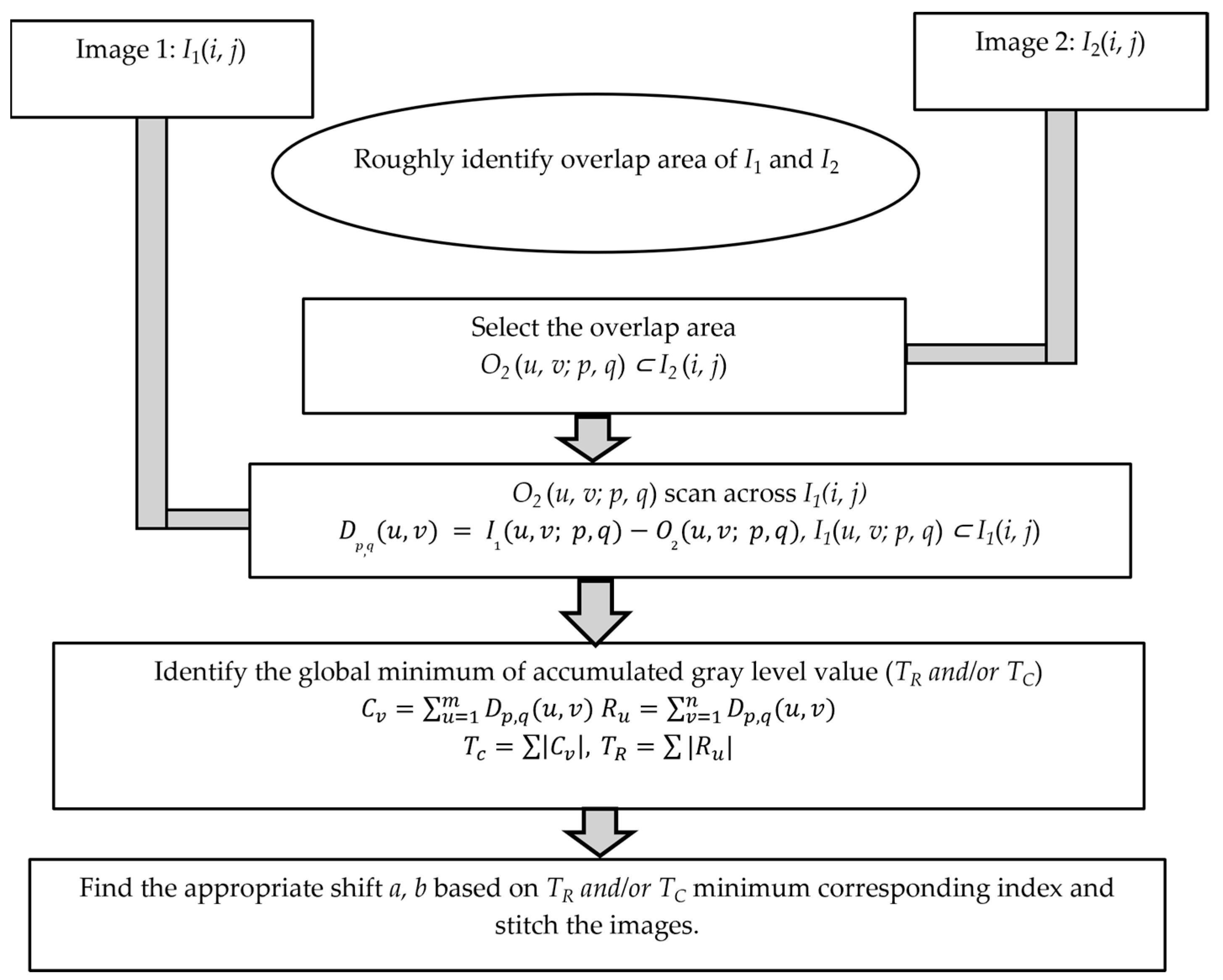
2.1. Pixel Level Image Registration

The SM was applied to perform image registration. A flowchart illustrating the resulting SM-based stitching process for two 1D images is shown in Figure 1. First, the two input images, each of size N by N, I₁ (i, j) and I₂ (i, j), are compared, where i ∈ [1, N], j ∈ [1, N]. An overlapped area of size m by n, defined as O₂ (u, v; p, q) with u ∈ [1, m], v ∈ [1, n] is selected within I₂ (i, j), i.e., O₂ (u, v; p, q) ⊂ I₂ (i, j). This overlapped area O₂ (u, v; p, q) is then scanned across the I₁ (i, j) with a step size of one pixel, where p and q represent the range of the sliding window in the x and y directions, respectively, with p ∈ [0, N$-$m] and q ∈ [0, N$-$n]. For each scanning step, the subtraction operation is computed as:

$$D_{p,q} (u, v)=I_1(u, v; p, q)-O_2(u, v; p, q)$$

Here, we use the estimation of the horizontal movement as an example; the size of O₂ (u, v; p, q) is selected to have the same number of rows as I₂ (i, j), i.e., m = N. This implies p = 0, meaning the window only scans across I₁ horizontally. It is clear that the choice of n has an impact on the size of O₂ (u, v; p, q), and consequentially, on computation time. The effects of this choice are discussed in detail in Section 3.2. This initial area can be determined in several ways: (i) by visual inspection or by reducing the total number of pixels in the image by generating super-pixels/increasing the pixelation; (ii) by performing an initial correlation calculation, which can be accelerated by using a reduced number of pixels, i.e., smaller local areas in the images, or by reducing the total number of pixels in the image by generating super-pixels/increasing the pixilation; or (iii) by repeated application of the SM by sliding the images together while ignoring non-overlapping regions. Afterwards, from D_p,q (u,v), two 1D vectors are generated, $C_v \mathrm{a}\mathrm{n}\mathrm{d} R_u$, by summing over the columns and rows, respectively:

$$C_v={\sum }_{u=1}^m{D}_{p,q}(u,v), R_u={\sum }_{v=1}^n{D}_{p,q}(u,v)$$

Adding the absolute values of the $C_v$ vector components and $R_u$ vector components, produces the scalars T_C, and T_R, respectively:

$$T_c=\sum \left|C_v\right|, T_R=\sum {|R}_u|$$

T_C and T_R have been repeatedly demonstrated to vary linearly with shifts in x (horizontal) and y (vertical) directions, respectively [13,14]. By evaluating these metrics as the overlapping area scans across the image with a step size of one pixel over the range of p and q, one can determine the location of optimal alignment. Specifically, the location corresponding to the minimum Tc indicates the best registration in the x direction, denoted as a. Similarly, the location of the minimum T_R in the y direction is denote as b. Note that for vertical movement, the size of O₂ (u, v; p, q) is different, where n = N, while the other procedures remain the same.

Based on this observation, the pixel position where T_R or T_C reaches its minimum corresponds to the best alignment, i.e., the closest image registration. Specifically, the position of the lowest T_C corresponding pixel value indicates the best alignment in the x direction while the lowest T_R corresponding pixel value indicates the best alignment in the y direction. The SM only requires low-complexity addition operations. However, both the initial identification of the overlapping area and the iterative process to achieve image registration can be time consuming. This process can be accelerated by (a) utilizing the availability of both T_R and T_C which permits nonlinear 2D gradient search routines to be employed [15,16,17] and (b) employing efficient computing implementations to speed up such searches [18,19].

To illustrate registration using the proposed SM, two 2D images were captured using a non-magnified 4-f imaging system as described in [13]. The object, A USAF chart [20], was moved parallel to the camera along both x and y directions. The results are shown in Figure 2, see the 1st and 2nd images (580 × 400 pixels, 16-bit gray level). The yellow boxes in the images indicate the overlap region (476 × 314 pixels). The overlap areas, i.e., O₂ (u, v; p, q), were selected within the yellow box, (Case 1: 200 × 200 pixels; and Case 2: 304 × 304 pixels) and the SM was applied. In both cases, the minimum values of T_C and T_R were identified to occur for a 96-pixel shift in x and 104-pixel shift in y. Using these values, the stitched image, having a combined total of 684 × 496 pixels, is shown in Figure 2. It is noted that the corresponding CM result was identical to the SM result.

The time taken by the CM for the full images using the MATLAB function fft2, ifft2, find, and conj command was 0.026 s. The time taken to perform the 2D search using the SM for Case 1 was 7.72 s, while for Case 2, it was 4.73 s. As can be seen, choosing a different size for the overlapped area O₂ (u, v; p, q) impacts the computational time. A more detailed analysis on time complexity between the CM and the SM can be seen in Section 3.2. The scan process involved only the use of “for loops” and no advanced search algorithm. All calculations were performed using MATLAB R2018a [21] installed on a computer with an Intel (R) Core (TM) i7-6700 CPU@3.40 GHz with 32 GB of RAM. We reduced the full 2D search above to two 1D searches by simply moving the overlapped area O₂ (u, v; p, q), in the x or y direction. The locations of the minimum values of T_C and T_R could always be identified, and for Case 1 (200 × 200 pixels), they had values at worst 1 pixel away from those found in the 2D case. The time taken to process these experimental data was 0.049 s.

2.2. Subpixel-Level Image Registration

To improve the quality of image stitching, subpixel registration is required. To do so, the image needs to be unsampled by interpolation. Before subpixel registration, the pixel level registration in the x or y directions must first be identified, as described in Section 2.1. First, the images with a size of N by N are interpolated by a factor of f, i.e., fN × fN. Since only a small portion of the original image is required to determine the subpixel shift, two small sub-areas I_1sub (i_sub, j_sub) and I_2sub (i_sub, j_sub) with a size of g by h are selected within I₁(i, j) and I₂(i, j), respectively. Similar to pixel-level registration shown in Figure 1, an overlap area is determined with a size m_sub by n_sub of O₂ (u_sub, v_sub; p_sub, q_sub), where p_sub ∈ [0, g-m_sub] and q_sub ∈ [0, h-n_sub]. By finding the corresponding pixel where T_R and T_c are minimum, similar to pixel-level registration, the subpixel level shifts in the x and y directions are found, here denoted as c and d, respectively. In this way, the total shift between two images can be determined with subpixel accuracy, i.e., a + c/f, b + d/f.

To illustrate this process, the 1st and 2nd images in Section 2.1 were upsampled by a factor of 10, using bicubic interpolation, resulting in images of size 5800 by 4000. The subsection area I_1sub (i_sub, j_sub) and I_2sub (i_sub, j_sub), each containing 512 × 512 values, were selected. By calculating the subpixel level shifts, 2 subpixels (equivalent in this case to 0.2 pixels) in x and 1 subpixel (equivalent in this case to 0.1 pixels) in y were identified. Therefore, the subpixel-accurate shifts between the original 1st and 2nd image were 96.2 pixels in x and 104.1 pixels in y, respectively.

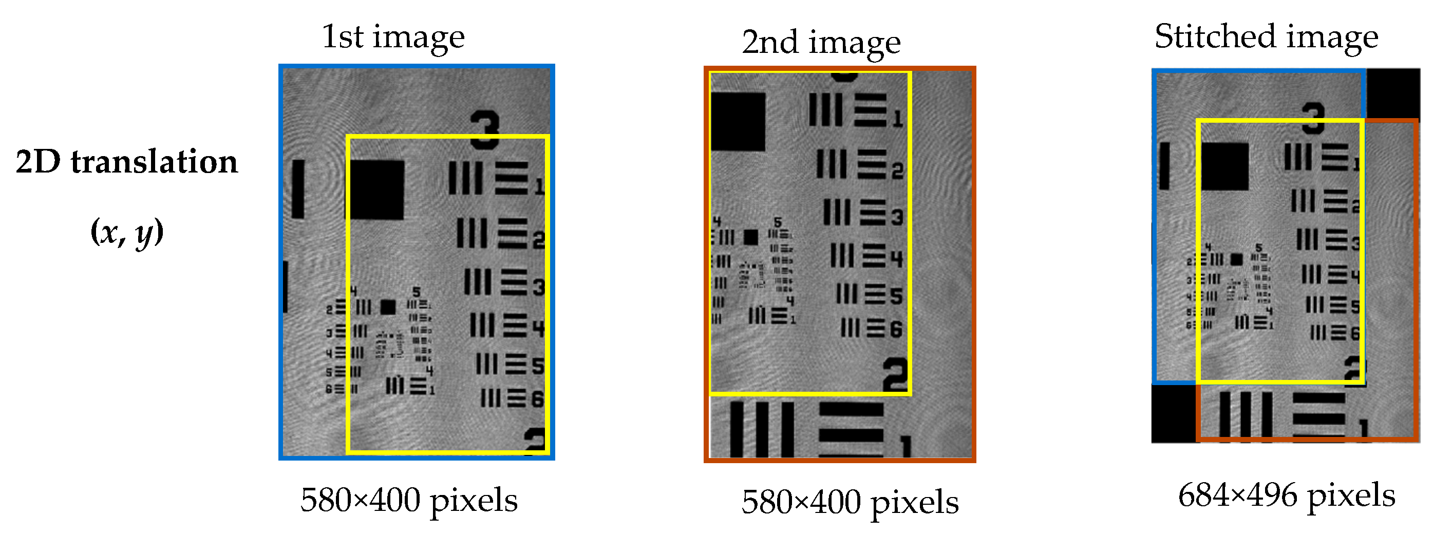
3. Holographic Imaging Stitching

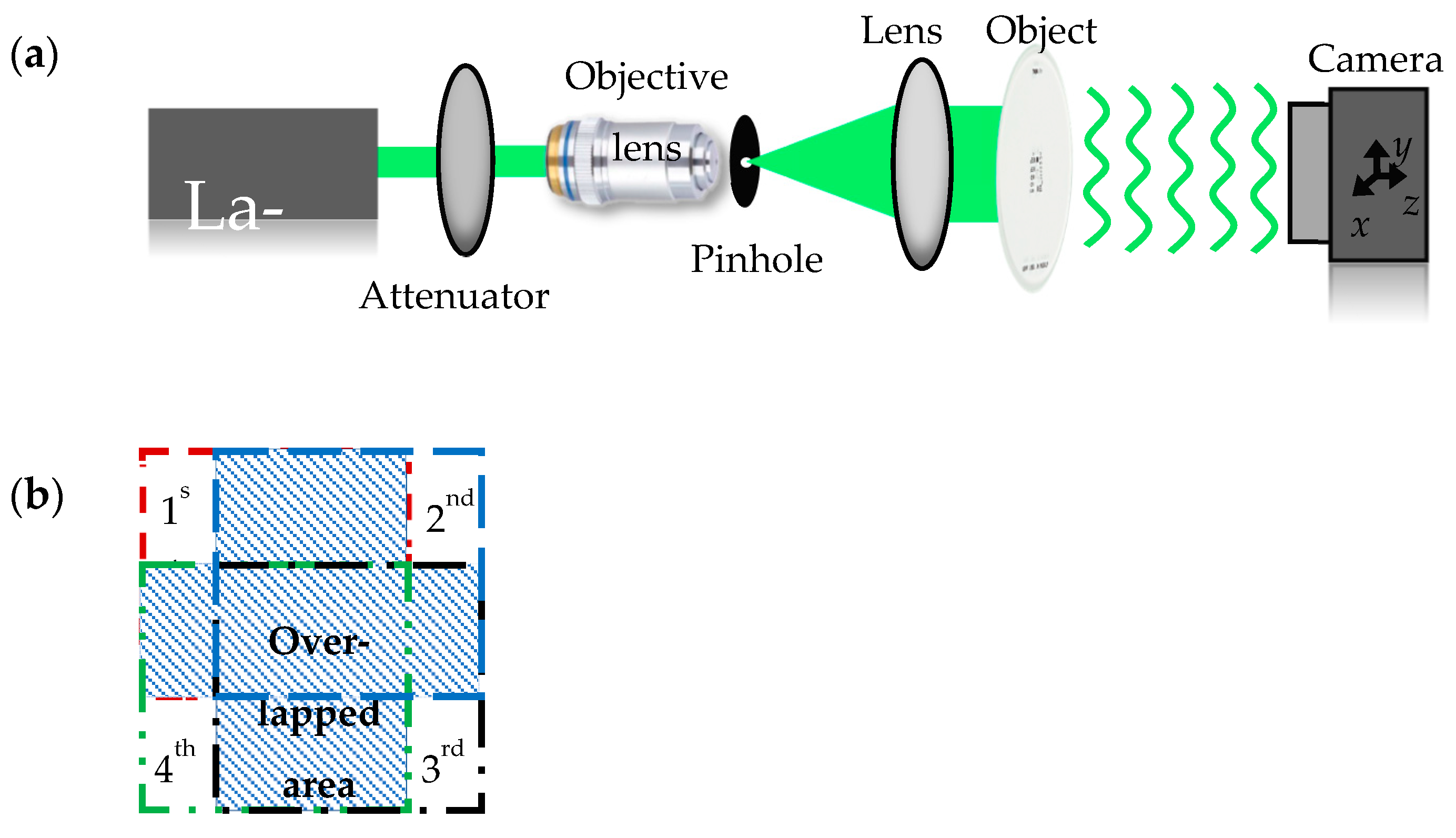
3.1. System Setup

To study the application of the SM to holographic data, an in-line digital holography system [22] was built using a diode pumped crystal laser (λ = 532 nm) and a Zyla 5.5 s CMOS camera (16-bit, 2160 × 2560 pixels, 6.5 µm pixel pitch, Oxford instruments Andor, UK), as shown in Figure 3a. The object was a 1951 USAF test target with external dimensions of 3.5 mm × 3.5 mm [20], which was illuminated by a plane wave. The camera position was altered using a 3D-translation stage [23], controlled by LabVIEW 2018 [24]. Each single hologram data array size was set and cropped to 1024 × 1024 pixels. Holograms were recorded at four different positions, as illustrated in Figure 3b. For each case, the background (without the object) was also recorded. The distance from the object to the camera was 42.8 cm.

3.2. Time Complexity Analysis

We compared the time complexity of the SM with that of other methods such as the CM, assuming a picture with a size of N by N. The CM has two types of variations, one based on convolution in the space domain with a time complexity of N⁴ [7] and another based on computation in the frequency domain, which has a time complexity of N²log₂N [25]. To ensure a fair comparison, we used the latter for the comparison with the SM.

The time complexity of the SM not only depends on the image size N but also on the size of O₂ (u, v; p, q). For example, for a horizontal movement only, the size of O₂ (u, v; p, q) has a size of m by n, where m = N, calculating D_p,q (u, v) has a time complexity of n × N, the calculation of C_v has a time complexity of n × N, and calculating T_c has a time complexity of n. However, this does not mean that defining a smaller n has less time complexity, since even though a smaller n reduces the size of O₂ (u, v; p, q), it also increase the number of scanning steps since more pixels need to be scanned by O₂ (u, v; p, q). The overall time complexity is (N − n) × (2nN + n).

The major limitation of the SM is that the subtraction operation is multiplied by the number of loop cycles, since O₂ (u, v; p, q) needs to be scanned across I₁ with a step size of a single pixel. This becomes even more problematic for larger image size. For example, a 4k image (3860 × 2010 pixels), as N increases, the SM has a much higher computation cost than the CM. However, this scanning process can be improved as it is unnecessary to scan I₁ pixel by pixel. An iterative optimization algorithm can be used to reduce the number of scanning steps, i.e., the term (N − n). The additional benefit of using an optimization algorithm is that a smaller n can be chosen, thereby further reducing the time complexity. Here, we used simulated annealing (SA) [26] combined with the SM (SMSA) to reduce the number of scanning steps. The number of iterations of SA depends on the annealing schedule; in our case, we defined the starting temperature at T_start = 25. For each iteration, the temperature was updated using a multiplicative cooling schedule. Specifically, the current temperature was multiplied by a cooling factor 0.9. The cooling terminated when T_end = 0.5. That means SA was run for 45 cycles. Since SA is sensitive to a given initial value, the initial value was estimated by sub-sampling D_p,q (u, v) at 30 pixel points that were evenly distributed points among N − n, and the pixel point that gave the lowest D_p,q (u, v) was selected as the starting point of the SA. Thus, the overall number of cycles was 75. When n = 100, the SMSA only required 8.11% of the original number of cycles of the SM.

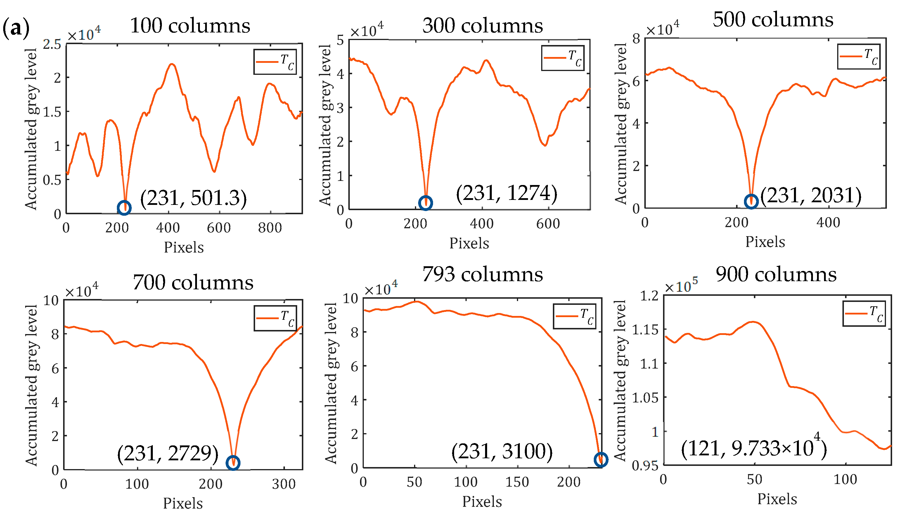
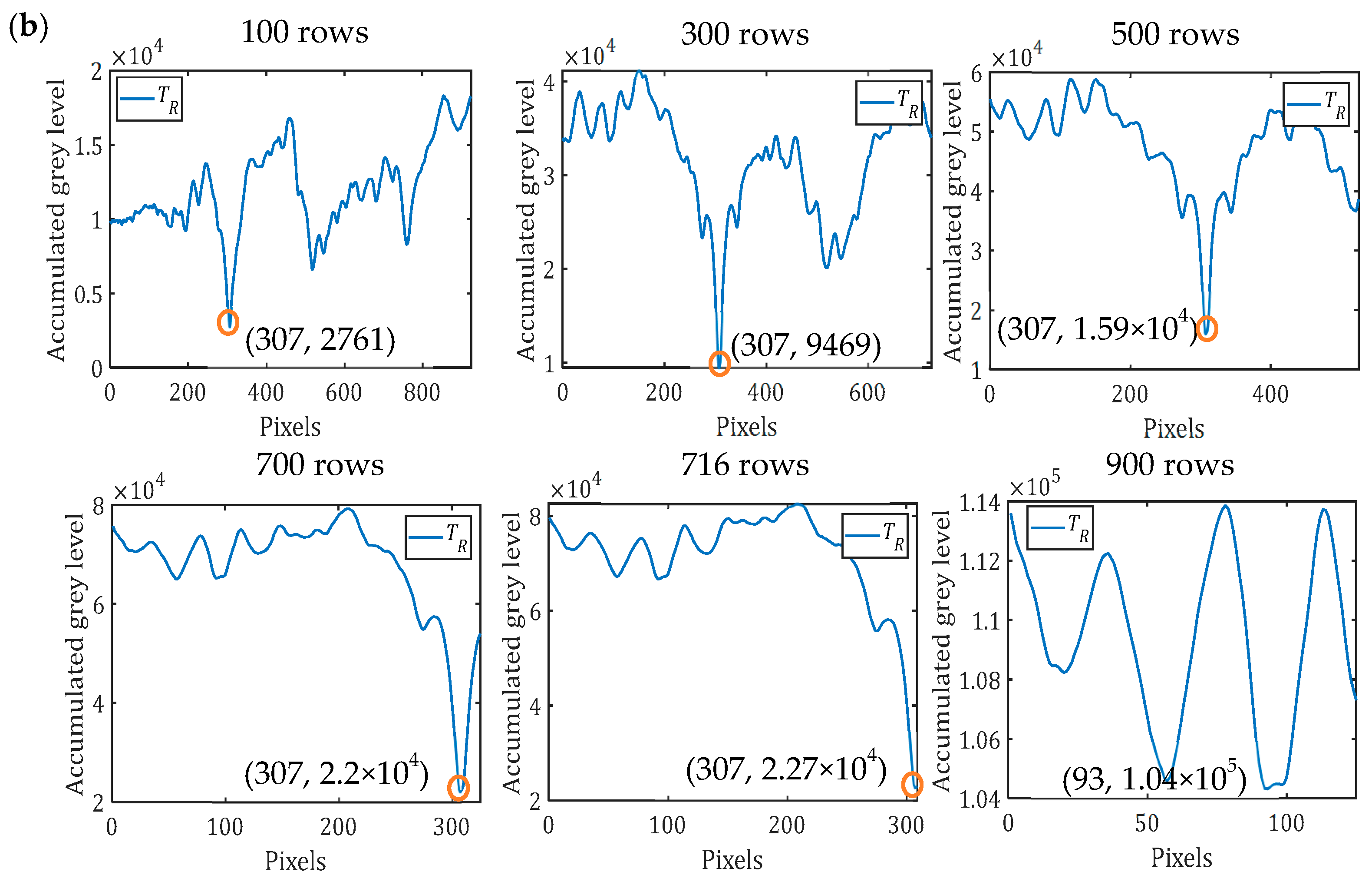
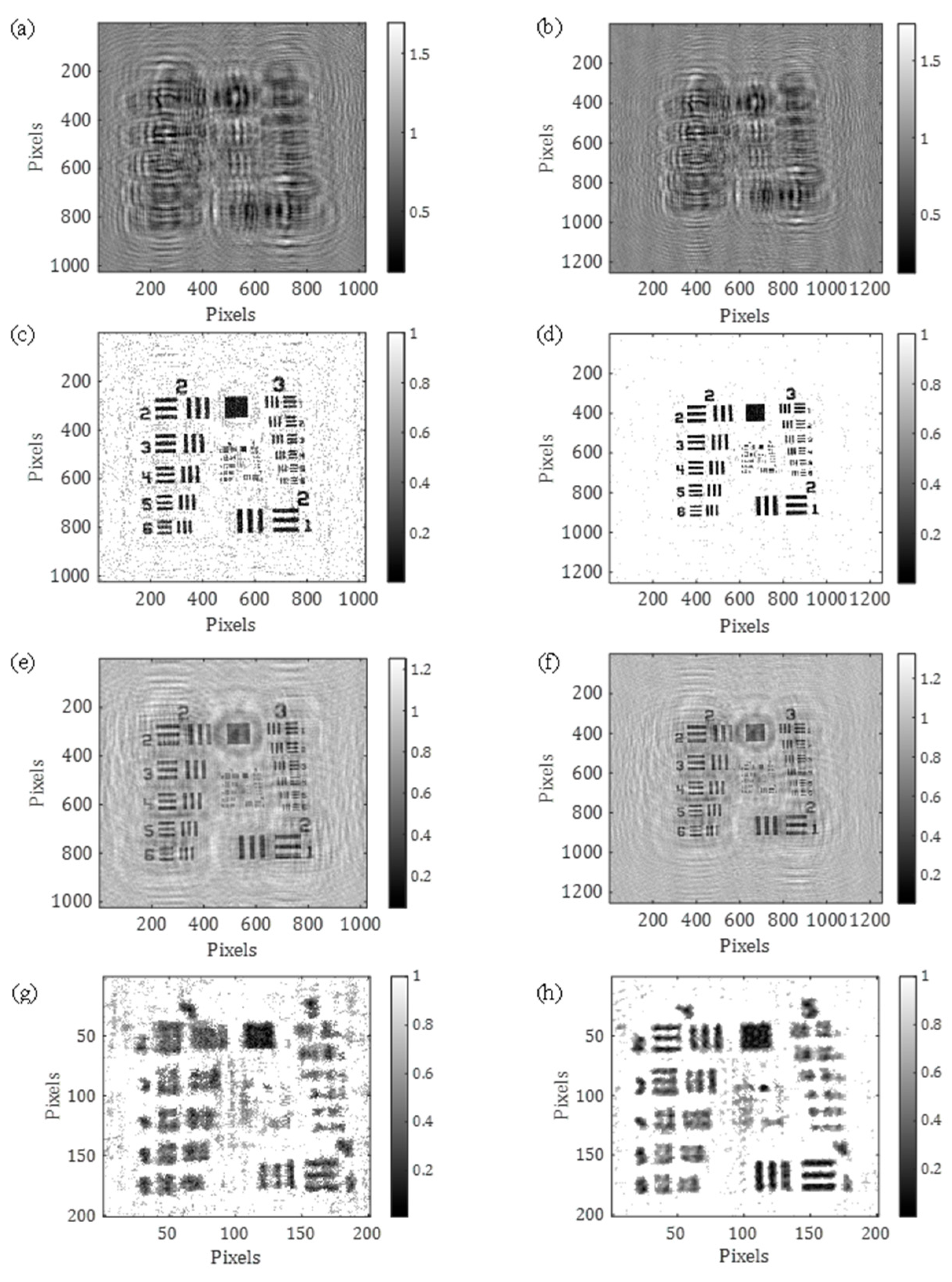
3.3. Pixel-Level Registration

To estimate the relative displacements between the four captured holograms, the SM was used. First, we tackled the pixel-level image registration problem. We examined the results for two cases in detail: first, a horizontal shift in x between the first and second holograms and second, a vertical shift in y between the first and fourth holograms. In the first case, the corresponding pixel position of the minimum T_C value was used to identify the horizontal shift in x. To do so, the subsection of the second hologram array data in the overlap area with the first hologram, as shown in Figure 3b, was scanned across the first hologram.

The corresponding T_C values are plotted in Figure 4a. Here, we chose five different values of n: 100, 300, 500, 700, and 793. The position of the lowest T_C value occurred at 231 pixels, as indicated in the first five figures in Figure 4a. However, if the selected number of columns exceeded the overlap area width, e.g., 900 columns, correct registration could not be performed, as shown in the sixth (last) figure in Figure 4a.

Similarly, the shifts in y between the first and fourth holograms were also calculated using the SM. In that case, we chose six different values for m, 100, 300, 500, 700, 715, and 900, to calculate T_R. A shift of 307 pixels between the two holograms was found. The corresponding results are shown in Figure 4b.

Next, we compared the computational time between the CM, the SM, and the SMSA. Additionally, we investigated the effect of m or n on the computation time. Here, we used the case of first and fourth holograms as an example, with m = 100, 300, 500, 700, 715, and 900. Results can be seen in

Table 1. Computational time of the CM, SM and SMSA with different values of m. Note that the CM is not dependent on the value of m, therefore the computational time theoretically remained the same regardless of the value of m for all cases.

	CM (ms)	SM (ms)	SMSA (ms)
m = 100	/	117	10.1
m = 300	/	138	12.2
m = 500	22.9	195	26.9
m = 700	/	169	37.3
m = 715	/	168	38.4
m = 900	/	96	55.2

. All calculations were performed using MATLAB R2023a on a 12th Gen Intel (R) Core(TM) i7-12700H 2.30 GHz with 16 GB of RAM.

From the computational time, it is clear that a small value of m was more beneficial for the SMSA since it led to a smaller size of O₂ (u, v; p, q). At m = 100, the SMSA required less computation time than the CM. However, from our observation, as m decreased beyond 100, the small size of O₂ (u, v; p, q) led to an incorrect pixel-shift estimation for the SMSA.

Examining all four overlap areas separately with the SM, the shifts between first and second, second and third, third and fourth, and first and fourth were 231 pixels, 308 pixels, 232 pixels, and 307 pixels, respectively. Furthermore, applying the SMSA with m or n = 100 yielded the same pixel shift. Once the relative shifts between the four holograms were identified, they could be combined to one single synthetic hologram having 1331 × 1254 pixels. A single central hologram, 1024 × 1024 pixels, centered on the overlap area, was captured for comparison. The single hologram and the synthetic hologram are shown in Figure 5a,b, respectively. As can be seen, the synthetic hologram contained more high-frequency information than the centered single hologram shown. The reconstructed results using the angular spectrum propagation algorithm [22] are shown in Figure 5c,d. The autofocusing algorithm [27] was used to obtain an accurate propagated distance, i.e., 42.8 cm. The phase retrieval algorithm [28] was used to eliminate the twin image. The reconstructed amplitude using the single and synthetic holograms are shown in Figure 5e,f. The subsection (highlighted by the red box) in Figure 5e,f is shown magnified in Figure 5g,h. We note that the times taken to perform the back propagation and phase retrieval in that case were 0.169 s and 63.38 s.

The reconstructed amplitudes were evaluated in comparison with the ideal USAF chart [20]. Several quantitative parameters were used: the Root-Mean-Square Deviation (RMSD) [29], Peak Signal-to-Noise Ratio (PSNR) [30], and image entropy (E) [31,32]. The E of Figure 5e,f and the RMSD and PSNR, of Figure 5g,h are summarized in Table 3 (Interpolation factor is one). All three metrics indicated that using the synthetic hologram provided better quality results than using the single central hologram. More noticeable visual differences can be seen in Figure 5g,h.

3.4. Subpixel-Level Registration

Next, we examined the subpixel-level registration problem in DH. Interpolation by a factor of two, four, and eight were applied to the experimental data presented in Figure 5a,b. Result from Section 3.3 shows that when m or n = 100, the SM and the SMSA required less computational time. The subpixel shift was calculated between the first and fourth holograms using m = 100 with a size of 256 by 256. The computational time is reported in

Table 2. Subpixel-level registration’s computational time with different interpolation factors.

Interpolation Factor	CM (ms)	SM (ms)	SMSA (ms)
2	6.927	20.71	3.842
4	23.78	147.2	12.74
8	101.2	843.6	31.23

.

For the subpixel level registration using the SM with interpolation factors of two, four, and eight, the shifts found between first and second holograms were 231.5, 231.25, and 231.12 pixels. Between the second and third holograms, the shifts were 308.5, 308.25, and 308.12 pixels. Between the third and fourth holograms, the shifts were 232.5, 232.25, and 232.12 pixels, and between the first and fourth holograms, they were 307, 306.75, and 306.62 pixels, respectively. These results demonstrate that subpixel registration was achieved. Similarly, the SMSA produced the same subpixel level shift results as the SM, confirming that the optimization could also be implemented at the subpixel level.

The reconstructed amplitudes at interpolation factors of two, four, and eight were compared to the ideal USAF chart [20]. The same three metrics were used: RMSD, PSNR, and E. The results are summarized in Table 3. All three metrics indicated that using the synthetic hologram provided better quality results than using the single central hologram for subpixel level registration. In addition, comparing these metrics with different interpolation factors, an improvement in image quality was observed.

Table 3. Subpixel level registration image metrics with different interpolation factors. An interpolation factor of 1 means there is only pixel-level registration.

Interpolation Factor	RMSD		PSNR		E
	Single	Synthetic	Single	Synthetic	Single	Synthetic
1	0.2766	0.2388	25.70	28.64	2.327	0.9938
2	0.2698	0.2367	26.20	28.81	2.316	0.9601
4	0.2681	0.2383	26.32	28.68	2.319	0.9582
8	0.2673	0.2401	26.38	28.50	2.310	0.9565

Table 3. Subpixel level registration image metrics with different interpolation factors. An interpolation factor of 1 means there is only pixel-level registration.

Interpolation Factor	RMSD		PSNR		E
	Single	Synthetic	Single	Synthetic	Single	Synthetic
1	0.2766	0.2388	25.70	28.64	2.327	0.9938
2	0.2698	0.2367	26.20	28.81	2.316	0.9601
4	0.2681	0.2383	26.32	28.68	2.319	0.9582
8	0.2673	0.2401	26.38	28.50	2.310	0.9565

4. Discussion

We verified the performance of the Subtraction Method (SM) for imaging registration with a variety of holographic images. Subsequently, we implemented and compared three different methods for pixel-level registration: the Correlation Method (CM), SM and Subtraction Method with simulated annealing optimization (SMSA). We investigated how the values of m or n impacted computational time, as summarized in Table 1. As expected, a large m or n increased the size of the overlapping region O₂ (u, v; p, q). Conversely, smaller values of m or n improved the computation speed of the SMSA but may increase the risk of an incorrect pixel-shift estimation. In addition, the computational time and accuracy of the SA depends on the cooling schedule. A more rapid cooling schedule reduces computation time but increases the risk of convergence to local minima [26]. Moreover, the performance of the SMSA is influenced by the initial value provided [33]; thus, careful tuning of the cooling schedule and proper selection of the initial value are essential for optimal performance. When comparing the computation time between the first and fourth holograms when m = 100, the SMSA was 11.58 times faster than the SM and 2.27 times faster than the CM. Importantly, the SMSA yielded the same shift value as the SM; thus, the SMSA reduced computational time without sacrificing the accuracy of the SM. Furthermore, for larger images, the SMSA can substantially reduce time complexity since the number of scanning steps of the SMSA is not limited by the image size N. Thus, only a relatively small overlap area O₂ (u, v; p, q). is sufficient to determine the pixel shift.

After stitching the holograms, we obtain the reconstructed amplitude through the angular spectrum propagation algorithm and iterative phase retrieval. Inspecting the reconstructed amplitudes in Figure 5g,h, it was evident that Figure 5h exhibited a lower noise level and higher spatial frequency information than Figure 5g. This observation was further supported by the metric values RMSD, PSNR and E, which demonstrated that Figure 5f aligned more closely with the ideal object.

Furthermore, we investigated the performance of the CM, SM, and SMSA at the subpixel level. By comparing computation times with different interpolation factors (two, four, and eight), as shown in Table 2, we found that the SMSA was faster than both the SM and the CM when n = 100. As the size of the calculated matrix depended on the interpolation factor, a higher interpolation factor resulted in better subpixel resolution but also increased computation time. For instance, doubling the interpolation factor resulted in a fourfold increase in the total number of image pixels. The implementation of the SMSA significantly reduced computational time while producing the same pixel shift. The implementation of the SMSA significantly reduced computational time, particularly for high-interpolation-factor subpixel registration. Additionally, the SMSA produced the same pixel shift as the SM, thereby confirming that it could be effectively implemented for subpixel-level registration. However, when comparing RMSD, PSNR, and E across different interpolation factors, we observed that while some improvements occurred as the interpolation factor increased, the differences became minimal beyond a factor of four, despite the additional computational cost. We attribute this to the nature of the reconstructed holographic images, which often contain large, smooth regions that limit the benefit of higher interpolation factors.

The SM achieved high accuracy in estimating pixel and subpixel shifts. With proper optimization such as the SMSA, it can achieve faster computational times than the CM. Future work will focus on the implementation of the SM and the SMSA in 2D pixel- and subpixel-level registration estimation instead of the current 1D direction stitching for hologram images. Another limitation is that the current SM does not account for rotational image registration. Therefore, implementing the SM to determine rotation and translation simultaneously is another attractive direction. To further explore the benefit of implementing the SM on holographic image registration at the subpixel level, we plan to evaluate its efficacy on images containing less-regular patterns and smoother regions. We believe that the SM can be used in applications that require high precision such as microscopic particle tracking [34], video analysis [35], remote sensing [35], structural dynamics analysis [36], and material science [37].

5. Conclusions

In this paper, we demonstrated the application of image registration using the Subtraction Method. Experimental data captured with a 4-f optical imaging system and in-line DH optical system were processed. Both pixel- and subpixel-level registration were examined. The computation time and resulting image quality were quantified. By incorporating the Subtraction Method with a simulated annealing optimization algorithm, the time taken to perform registration was 2.5 times faster than the correlation method, without compromising pixel-shift estimation accuracy. After stitching the hologram with the SM, the reconstructed images were compared with a single image. In all cases, the image quality of synthetic aperture images was enhanced.

References

1. Szeliski, R. Image Alignment and Stitching: A Tutorial. Found. Trends Comput. Graph. Vis. 2007, 2, 1–104. [Google Scholar] [CrossRef]
2. Brown, L.G. A Survey of Image Registration Techniques. ACM Comput. Surv. 1992, 24, 325–376. [Google Scholar] [CrossRef]
3. Adel, E.; Elmogy, M.; Elbakry, H. Image Stitching Based on Feature Extraction Techniques: A Survey. Int. J. Comput. Appl. 2014, 99, 1–8. [Google Scholar] [CrossRef]
4. Levin, A.; Zomet, A.; Peleg, S.; Weiss, Y. Seamless Image Stitching in the Gradient Domain. Computer Vision—ECCV. 2004, 3024, 377–389. [Google Scholar]
5. Megha, V.; Rajkumar, K.K. A Comparative Study on Different Image Stitching Techniques. Int. J. Eng. Trends Technol. 2022, 70, 44–58. [Google Scholar]
6. Xiong, Y.; Turkowski, K. Registration, Calibration and Blending in Creating High-Quality Panoramas. In Proceedings of the Fourth IEEE Workshop on Applications of Computer Vision (WACV’98), Princeton, NJ, USA, 19–21 October 1998; pp. 69–74. [Google Scholar]
7. Rankov, V.; Locke, R.J.; Edens, R.J.; Barber, P.R.; Vojnovic, B. An Algorithm for Image Stitching and Blending. In Proceedings of the SPIE in Three-Dimensional and Multidimensional Microscopy, San Jose, CA, USA, 22–27 January 2005; Volume 5701, pp. 190–199. [Google Scholar]
8. Wan, M.; Healy, J.J.; Sheridan, J.T. Fast 2D Subpixel Displacement Estimation. Photonics 2024, 11, 625. [Google Scholar] [CrossRef]
9. Goodman, J.W. Introduction to Fourier Optics, 3rd ed.; Roberts and Company: Greenwood Village, CO, USA, 2005. [Google Scholar]
10. Schnars, U.; Falldorf, C.; Watson, J.; Jüptner, W. Digital Holography and Wavefront Sensing: Digital Holography; Springer: Berlin/Heidelberg, Germany, 2015; pp. 39–68. [Google Scholar]
11. Rivenson, Y.; Wu, Y.; Ozcan, A. Deep Learning in Holography and Coherent Imaging. Light Sci. Appl. 2019, 8, 85. [Google Scholar] [CrossRef]
12. Zhang, W.; Cao, L.; Jin, G. Review on High Resolution and Large Field of View Digital Holography. Infrared Laser Eng. 2019, 48, 603008. [Google Scholar]
13. Wan, M.; Healy, J.J.; Sheridan, J.T. Fast, Sub-Pixel Accurate, Displacement Measurement Method: Optical and Terahertz Systems. Opt. Lett. 2020, 45, 6611–6614. [Google Scholar] [CrossRef]
14. Wan, M.; Healy, J.J.; Sheridan, J.T. Fast subpixel displacement measurement, part 1: One-dimensional analysis, simulation, and experiment. Opt. Eng. 2022, 61, 043105. [Google Scholar] [CrossRef]
15. Nocedal, J.; Wright, S.J. Numerical Optimization; Springer Science & Business Media: Berlin/Heidelberg, Germany, 2006. [Google Scholar]
16. Ahmadianfar, O.; Bozorg-Haddad, O.; Chu, X. Gradient-Based Optimizer: A New Metaheuristic Optimization Algorithm. Inf. Sci. 2020, 540, 131–159. [Google Scholar] [CrossRef]
17. Standford AAA222 Lecture 3 Note. Available online: https://office365stanford-my.sharepoint.com/ (accessed on 19 March 2025).
18. Why Your Loops Are So Slow. Available online: https://medium.com/data-science/why-your-loops-are-so-slow-166ec67db47d (accessed on 19 March 2025).
19. Cooper, K.; Torczon, L. Engineering a Compiler: Introduction to Optimization; Elsevier: Amsterdam, The Netherlands, 2011; Chapter 8. [Google Scholar]
20. RQDS1P-Positive 1951 USAF Test Target Groups 2–7. Available online: https://www.thorlabs.com/thorproduct.cfm?partnumber=R1DS1P (accessed on 19 March 2025).
21. MATLAB 2018a. Available online: https://nl.mathworks.com/downloads/ (accessed on 26 May 2025).
22. Wan, M.; Yuan, H.; Čibiraitė, D.; Cassidy, D.; Lisauskas, A.; Healy, J.J.; Roskos, H.G.; Krozer, V.; Sheridan, J.T. Terahertz Quantitative Metrology Using 300 GHz In-Line Digital Holography. Proc. SPIE 2019, 11030, 110300R. [Google Scholar]
23. 8MT167-100—Motorized Translation Stage. Available online: http://www.standa.lt/products/catalog/motorised_positioners?item=64 (accessed on 19 March 2025).
24. LabVIEW. Available online: https://www.ni.com/en-ie/support/downloads/software-products/download.labview.html#411240 (accessed on 19 March 2025).
25. Sundararajan, D. Digital Image Processing: A Signal Processing and Algorithmic Approach; Springer: Singapore, 2017; Chapter 3.3. [Google Scholar]
26. Kirkpatrick, S.; Gelatt, C.D.J.; Vecchi, M.P. Optimization by Simulated Annealing. Science 1983, 220, 671–680. [Google Scholar] [CrossRef]
27. Lyu, M.; Yuan, C.; Li, D.; Situ, G. Fast Autofocusing in Digital Holography Using the Magnitude Differential. Appl. Opt. 2017, 56, F152–F157. [Google Scholar] [CrossRef]
28. Latychevskaia, T. Iterative Phase Retrieval for Digital Holography: Tutorial. JOSA A 2019, 36, D31–D40. [Google Scholar] [CrossRef]
29. Wikipedia. Root-Mean-Square Deviation. Available online: https://en.wikipedia.org/wiki/Root-mean-square_deviation (accessed on 19 March 2025).
30. Wikipedia. Peak Signal-to-Noise Ratio. Available online: https://en.wikipedia.org/wiki/Peak_signal-to-noise_ratio (accessed on 19 March 2025).
31. Tsai, D.Y.; Lee, Y.; Matsuyama, E. Information Entropy Measure for Evaluation of Image Quality. J. Digit. Imaging 2008, 21, 338–347. [Google Scholar] [CrossRef]
32. Entropy. Available online: https://uk.mathworks.com/help/images/ref/entropy.html (accessed on 19 March 2025).
33. Kolonko, M. Some New Results on Simulated Annealing Applied to the Job Shop Scheduling Problem. Eur. J. Oper. Res. 1999, 113, 123–136. [Google Scholar] [CrossRef]
34. Memmolo, P.; Miccio, L.; Paturzo, M.; Di Caprio, G.; Coppola, G.; Netti, P.A.; Ferraro, P. Recent Advances in Holographic 3D Particle Tracking. Adv. Opt. Photon. 2015, 7, 713–755. [Google Scholar] [CrossRef]
35. Paul, M.; Lin, W.; Lau, C.T.; Lee, B.S. Direct Intermode Selection for H.264 Video Coding Using Phase Correlation. IEEE Trans. Image Process. 2010, 20, 461–473. [Google Scholar] [CrossRef]
36. Baqersad, J.; Poozesh, P.; Niezrecki, C.; Avitabile, P. Photogrammetry and Optical Methods in Structural Dynamics—A Review. Mech. Syst. Signal Process. 2017, 86, 17–34. [Google Scholar] [CrossRef]
37. Li, J.; Thakur, P.; Fok, A.S.L. Shrinkage of Dental Composite in Simulated Cavity Measured with Digital Image Correlation. JoVE J. Vis. Exp. 2014, 89, 51191. [Google Scholar]
Figure 1. Flow diagram of the SM for pixel-level image registration.
Photonics 12 00551 g001
Figure 2. Imaging stitching with pixel-level registration. The yellow box indicates the overlapped area of the 1st and 2nd image.
Photonics 12 00551 g002
Figure 3. (a) The schematic of the in-line digital holography system. (b) Positions of four captured holograms. The 1st hologram (red) is horizontally aligned with the 2nd hologram (blue). The 1st hologram (red) and 4th hologram (green) are vertically aligned. The 4th (green) and 3rd hologram (black) are horizontally aligned.
Photonics 12 00551 g003
Figure 4. The position of (a) the minimum of the TC values for the 1st and 2nd holograms; and (b) the minimum of the TR values for the 1st and 4th holograms. The minimum values of accumulated grey level and its corresponding pixel shifts are identified and marked as circles.
Photonics 12 00551 g004aPhotonics 12 00551 g004b
Figure 5. The results of in-line holography: (a) the single central and (b) synthetic holograms; (c) and (d) the amplitude of the object reconstructed by backpropagation using the angular algorithm [22] using (a,b), respectively. (e,f) Resulting amplitudes of the object, following 100 iterations, reconstructed using phase retrieval [28]. (g,h) Central subsections of (e,f) containing 200 × 200 pixels.
Photonics 12 00551 g005