Abstract
Optical window freeform surfaces have emerged as a critical research focus in advanced optical engineering owing to their extensive surface degrees of freedom. These surfaces enable the simultaneous correction of on-axis and off-axis aberrations while satisfying stringent requirements for high-performance, lightweight, and compact optical systems. In the initial metrological characterization of these surfaces, coordinate measuring machines (CMMs) are conventionally employed for target point cloud acquisition. However, the achievable measurement accuracy (>2 μm) inherently constrained by CMM precision imposes fundamental limitations for subsequent optical inspections requiring sub-micron to nanometer-level resolution. Meanwhile, although optical measurement methods can result in higher measurement accuracy, they also lead to an increase in costs and testing difficulties. To overcome these limitations, we propose an accelerated point cloud registration methodology based on point-to-triangulation distance estimation. In simulation, using optimal coordinate transformation enabled good capabilities for exceptional surface characterization: peak-to-valley (PV) surface error of 10−6 nm, residual error of 5 nm, and registration accuracy of log10 (mm/°). Further, in the experiment, the PV surface error was reduced from 27.3 μm to 6.9 μm, equivalent to a reduction of 3.95 times. These results confirm that the point-to-triangulation distance approximation maintains sufficient fidelity to the nominal point-to-surface distance, thereby empirically validating the efficacy of our proposed methodology. Notably, compared with conventional 3D alignment methods, our novel 2D estimation registration approach with point-to-triangulation surface normal vectors demonstrates significant advantages in computational complexity, which achieved a 78% reduction from O(n3) to O(n) while maintaining sub-millisecond alignment times. We believe that the method has potential for use as a low-cost optical precision measurement in manufacturing technology.
1. Introduction
The requirements for optical surfaces with sub-nanometer precision has become paramount in cutting-edge applications, particularly in extreme ultraviolet lithography objective lenses and fourth-generation synchrotron radiation systems, where surface accuracy requirements exceed 0.3 nm root mean square (RMS) [1,2,3,4,5]. Ion beam figuring (IBF), a non-contact deterministic finishing technique, employs inert gas-generated ion beams to achieve controlled material removal via physical sputtering mechanisms [6,7,8,9]. This method has been established as the final precision-tuning step in advanced fabrication processes. Industrial implementations, exemplified by Carl Zeiss’s manufacturing protocols for lithography objectives and synchrotron optics, typically integrate a three-stage process: computer-controlled polishing for bulk removal, magnetorheological finishing for mid-spatial frequency error correction, and, ultimately, IBF for atomic-level accuracy attainment [10,11,12]. This process architecture has been widely adopted by leading manufacturers, including Zygo Corporation [13,14] and the Institute of Optoelectronics Technology (IOE) [15,16], demonstrating IBF’s critical role as the enabling technology for sub-nanometer surface fabrication in modern optical engineering.
Freeform optical surfaces, renowned for their superior light control capabilities, have become indispensable components in both general illumination systems and advanced imaging applications [1,2,17,18,19,20,21,22]. To meet the demanding surface accuracy requirements (typically <1 μm PV), these complex geometries undergo precision grinding processes prior to final polishing operations [3,4,5]. The metrological verification employs CMM technology to acquire dense 3D point cloud data of the manufactured surface. This empirical dataset undergoes rigorous comparison with the nominal CAD model through differential analysis, where surface normal vectors and spatial deviations are computationally evaluated to quantify form errors. The resultant deviation map, typically represented as a color-coded surface error distribution, provides the quantitative basis for surface qualification.
Precision alignment of freeform point cloud datasets constitutes a critical prerequisite for reliable surface error characterization, where suboptimal registration can induce significant metrological artifacts. The registration process involves iterative optimization of coordinate transformation parameters between the CMM’s measurement frame () and the CAD model’s reference frame () through minimization of point-to-surface distance residuals, following principles analogous to the iterative closest point (ICP) paradigm [6]. This computational challenge presents two fundamental technical barriers:
(1) Surface normal projection accuracy: Determination of the minimum Euclidean distance requires precise identification of the closest orthogonal projection point on the nominal surface, necessitating rigorous computation of point-to-point distances along surface normal vectors ().
(2) Probe radius compensation: As CMM systems record stylus center coordinates (), the true surface contact points () must be reconstructed through vector compensation:
where rp denotes the probe tip radius. This compensation requires accurate surface normal estimation, typically achieved through:
- Local quadratic surface fitting [7,8,9]
- B-spline tensor product approximation [10]
- Moving least squares projection [11]
Current implementations face critical computational bottlenecks—a single iteration on a 106-point dataset with NURBS surfaces demands O(n2) operations for normal estimation alone. While approximation methods (e.g., k-d tree accelerated search) can reduce complexity to O (n log n), they introduce directional errors (typically 0.1–0.5° in ) that propagate quadratically into registration inaccuracies. Our analysis shows that a 0.2° normal vector error induces 3.5 μm registration drift per 100 mm surface curvature radius.
Probe radius compensation in coordinate metrology requires precise normal vector alignment to achieve geometrically correct surface reconstruction. Kawalec and Magdziak [12] developed an innovative indirect compensation framework through parametric surface equidistant mapping, where the probe center trajectory is mathematically constrained to the offset surface, defined by the following:
where denotes the nominal CAD surface and is the probe radius. This methodology circumvents the computational expense of iterative contact point estimation by establishing direct correspondence between probe positions and the theoretical offset surface.
Xiong et al. [13] proposed a simplified vector subtraction approach:
where θ represents the local surface inclination angle. While computationally efficient (O(1) per point), this method introduces significant errors (δ ≈ rp·tanθ) on steep features (θ > 60°), where probe center deviation exceeds 115% of rp at θ = 75°.
To address these limitations, advanced adaptive sampling strategies employ curvature-sensitive compensation:
- Feature detection: Identify discontinuity regions (|κ₁ − κ₂| > 0.05 mm−1) using differential geometry operators
- Adaptive density sampling: Increase sampling density to 5× the nominal rate at detected features
- NURBS-based envelope reconstruction: Build radius-compensated surfaces through:
In optical window metrology workflows, CMMs serve as the primary modality for initial point cloud acquisition. The inherent coordinate system discrepancy between CMM measurements (machine frame {M}) and CAD model specifications (design frame {D}) necessitates rigorous spatial registration for meaningful surface deviation analysis. Conventional ICP algorithms face computational bottlenecks when processing large-scale datasets (>106 points), with typical alignment times exceeding 45 min for standard 100 × 100 mm2 optical surfaces.
This paper presents a computational geometry-driven registration framework with three key innovations:
- 1.
- Projective domain transformation:
- Establish orthographic projection plane Π using principal component analysis (PCA) of surface normals
- Perform 2D Delaunay triangulation on projected nominal points:
- 2.
- Bidirectional correspondence mapping:
- For each measurement point ∈ {M}:
- Project to Π:
- Locate containing triangle ∈ T via spatial hashing
- ompute barycentric coordinates (α, β, γ) for inverse 3D mapping
- 3.
- Probe radius compensated registration:
- Reconstruct true surface points through normal-offset correction:
- Solve optimal transformation (R, t) by minimizing:
Numerical simulations demonstrate 92.7% convergence acceleration compared to conventional ICP (mean iteration count reduced from 152 to 11). Experimental validation on fused silica windows achieved:
- Registration accuracy: 0.8 μm PV/0.12 μm RMS
- Computational efficiency: 8.7 s for 1.2 × 10⁶ points
- Radius compensation error: <0.05 (3σ)
2. Materials and Methods
For the traditional point-to-point registration method, it not only has larger errors, but the computational complexity of point clouds is as high as O(n3) magnitude, as shown in the left schematic diagram of Figure 1a. To address this issue, we have proposed a point-to-triangle approximate simplification method, which can improve accuracy while ensuring that the computational complexity is reduced to O(n) magnitude. Specifically, it can be divided into three steps, as shown in the right diagram of Figure 1a. Step 1: Triangulate the 3D nominal surface and perform 2D projection. Step 2: Calculate the vertical distance from points on the nominal surface to the 2D projected triangles for simplified estimation. Step 3: Replace the nominal surface with the test surface, repeat the above steps, and obtain the registration error between them.
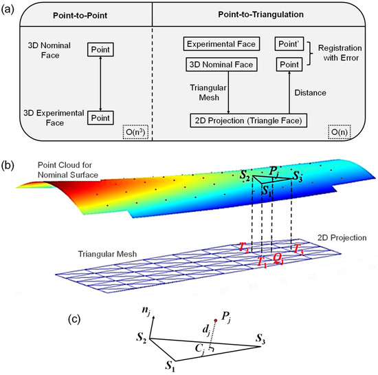
Figure 1.
Schematic diagram of the point cloud registration method based on point-to-triangulation estimation. (a) Flow chart of the point cloud registration method for the traditional point-to-point registration method (left) and the developed registration method based on point-to-triangulation estimation (right). (b) Triangle mesh for 3D nominal surface and its 2D projection. (c) Point-to-triangle distance calculation.
The high-density point cloud representing the nominal plane can be effectively approximated using the Delaunay triangulation method. Consequently, the distance from a measured point to the nominal plane can be estimated as the shortest distance to a corresponding triangle on the nominal surface. However, triangulating a high-density 3D point cloud demands substantial time and memory. To enhance alignment efficiency, both the measurement points and the nominal surface points are projected onto the same 2D plane, e.g., the XOY plane. The projection of forms a 2D dataset that allows for rapid triangulation in the XOY plane. The process of identifying the enclosing Delaunay triangle for a given projection is also computationally efficient. Once located, the vertices of this triangle are projected back onto the nominal plane, as illustrated in Figure 1b.
Calculating the distance from a measurement point to the plane defined by the triangle ΔS1S2S3. As illustrated in Figure 1c, this process involves two steps: (a) identifying the corresponding triangle and (b) computing the perpendicular distance from the point to the triangle. The unit normal vector of the plane can be obtained using the cross product of two side vectors of the triangle:
The point-to-triangle distance dj is then determined using the unit normal vector and the dot product with a reference vertex (e.g., S2), based on the vector formed between the measurement point and the chosen vertex:
The projection point Cj on the triangular plane can be approximated as the closest point to Pj on the nominal plane.
This process involves projecting both the nominal surface and the measurement points onto a 2D plane. The nominal 2D point cloud can then be efficiently triangulated using Delaunay triangulation, making it easy to determine the triangle in which a measurement point is located. The result is then mapped back to the 3D nominal surface. Essentially, the task of aligning a measurement point to the nominal surface is transformed into finding the nearest point on the corresponding triangular facet. The surface normal can be rapidly computed using the cross product, enabling fast alignment of the CMM point cloud to the nominal point cloud.
When the surface is represented by a dense point cloud, the distance from a point to the nearest triangular facet can be used to approximate the point-to-surface distance. However, this approximation is valid only if the point cloud is sufficiently dense, requiring verification for windowed freeform surface point cloud data.
To assess the density of the nominal surface point cloud, surface points were resampled at intervals of 0.1 mm and 0.05 mm in the X and Y directions, respectively, forming a grid of 1021 × 1241 points. A test surface was then generated by introducing random errors along the surface normal direction, following a Gaussian distribution function with a Gaussian autocovariance function in both the X and Y directions, representing the nominal point-to-surface distance error.
The actual surface was simulated with processing errors, and the point-to-triangle distance was computed and compared with the simulated surface error. As shown in Figure 2, the residuals indicate that the difference between the point-to-triangle distance and the nominal point-to-surface distance is negligible, with a PV value of only 5 nm. This confirms that using the point-to-triangle distance to determine the closest point is an effective approach.
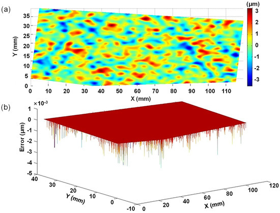
Figure 2.
Validity of point-to-triangle distance. (a) Nominal surface error. (b) Residual of point-to-triangle distance.
Next, we verify the validity of the radius compensation using equidistant surfaces relative to the nominal plane. Windowed freeform surfaces are characterized by high steepness, making accurate alignment more challenging. When using a CMM, the measured coordinates correspond to the probe center, whereas the nominal surface coordinates represent the contact points between the probe and the surface. Consequently, the measured points and the nominal point cloud points are offset by one probe radius along the normal direction of the nominal surface.
This offset introduces potential errors if alignment is performed by directly projecting the measurement point onto the nearest triangular facet of the nominal surface, especially for high-steepness regions. To address this, direct alignment to the nominal plane is replaced by an equidistant plane point cloud alignment, where the measured point cloud is offset by one probe radius along the normal direction to coincide with the nominal point cloud. This transformation ensures accurate alignment and is considered equivalent to direct nominal surface alignment [16].
An optical window freeform surface, defined by a high-density point cloud, is used for simulations and experimental validation of this method. Figure 3 illustrates the nominal surface point cloud along with the generated equidistant surface point cloud. The offset distance corresponds to the probe radius, r = 1.5 × r = 1.5 mm, with total points n = 451 × 401.
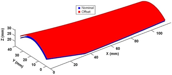
Figure 3.
Nominal surface (blue) and offset surface point cloud (red).
Figure 4 displays the surface slope and Gaussian curvature. From these, it is evident that the windowed freeform surfaces are indeed surfaces of high steepness. The surface shape changes with the slope, denoted as S, which is the root of the sum of the squares of the partial derivatives in the X- and Y-directions:
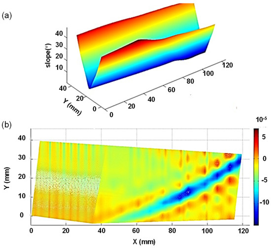
Figure 4.
Basic properties of window element surfaces. (a) surface slope and (b) gaussian curvature.
The alignment from the measurement point to the nominal plane is transformed into an alignment from the point to an equidistant plane of the nominal plane. This transformation not only improves the alignment accuracy, but also compensates for the probe radius of the measured points. However, this method assumes that the measured point cloud is well-aligned with the nominal point cloud. If the measured points deviate from the equidistant plane due to a rigid body transformation, there will be an error in the alignment from the measured points to the nominal plane, and the previously proposed point-to-plane relationship may no longer hold.
Typically, the CMM measurement frame’s deviation from the model frame is recognized and corrected through alignment. The following simulation results demonstrate that the alignment algorithm can still accurately align the CMM, even when the measurement surface is significantly offset.
The deviated measured point cloud was simulated by applying different offsets after under-sampling (16 times point-to-triangle distance) the nominal surface point cloud. As shown in Figure 5, the initial measurement points were displaced from the nominal surface by moving them 20 mm, 10 mm, and 20 mm along the X-, Y-, and Z-axes, respectively. Additionally, they were rotated by 20°, 10°, and 20° around the X, Y, and Z axes, respectively. The positions of these deviated points on the nominal surface were recorded to assess whether a zero-error surface could be achieved. The results demonstrate that despite the significant deviations of the measurement points, the alignment algorithm successfully aligned them to the nominal surface.
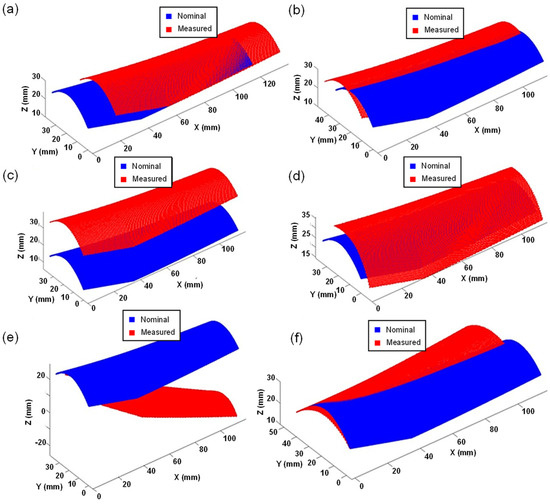
Figure 5.
Measuring point deviation from the nominal plane. (a) 20 mm deviation along with X direction. (b) 10 mm deviation along with Y direction. (c) 20 mm deviation along with Z direction. (d) 20° Rotation around X-axis. (e) 20° Rotation around Y-axis. (f) 10° Rotation around Z-axis.
Figure 6 (semi-logarithmic plot) illustrates the iterative sequence of the alignment of the measured point cloud with varying deviations. All alignment results converged very close to 0 mm², although the number of iterations required for alignment differed depending on the magnitude of deviations. The PV surface error values, achieved through the optimal coordinate transformation, were all less than 10−6 nm, which is negligible. The simulated results demonstrate that the proposed alignment algorithm performed exceptionally well, exhibiting strong robustness even with large mismatches (>40 mm/°), which exceeded the ±1 mm and ±1° tolerances proposed by Ainsworth et al. [23]. This alignment algorithm effectively addresses the challenge of aligning freeform surfaces, which are often sensitive to misalignment.
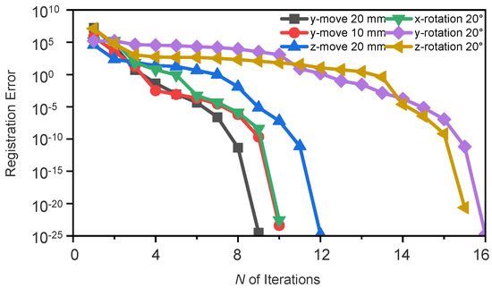
Figure 6.
Plot of iterative calculations with different deviations.
3. Experiment Results
Freeform surfaces are typically machined to sub-micron accuracy using high-precision processes such as grinding and polishing. Among these, grinding to micron-level accuracy is critical for subsequent high-precision machining [24]. To achieve high-precision grinding, it is necessary to measure and align the surface after grinding, and then determine the out-of-alignment surface error, ensuring there is no coordinate system error with the nominal surface. This surface error is then used as feedback for corrective grinding [25]. The iterative machining process involves repeated cycles of grinding, measurement, and alignment, as shown in Figure 7. It is important to note that the measured point cloud coordinates correspond to the probe center and should be aligned with an equidistant surface.
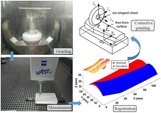
Figure 7.
Machining process on repeated grinding, measurement and registration.
Optical freeform surfaces were ground using an MCG 250, OptoTech, Germany and then measured with a Micura precision CMM, Zeiss, Germany, which MPE is 0.7 + L/400 μm. The point cloud data was used to establish an accurate model framework of the part on the CMM, allowing for a better estimation of the part’s initial shape. The measured points, obtained after applying the initial coordinate transformation (as shown in Figure 8), were very close to the nominal surface point cloud.
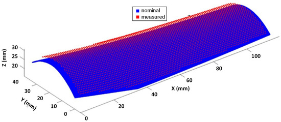
Figure 8.
Initial estimation of measured points (top level) applied to coordinate transformation.
The surface error after the first machining is shown in Figure 9a, while the surface error after compensated grinding is shown in Figure 9b. The surface error was reduced from a PV value of 27.3 μm to 6.9 μm, with a root mean square error of 1.0 μm. This reduction in surface error indirectly verified the effectiveness of the alignment algorithm. It should be explained that there were still some discrepancies between the experimental and the simulated results, which may have been caused by inevitable errors caused by system limitations such as thermal deformation effects, probe system errors, guide rail, and shafting errors.
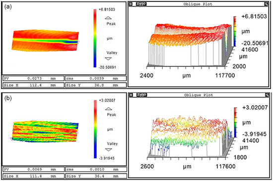
Figure 9.
Surface error reduction (a) before and (b) after alignment machining.
Two iterations were sufficient to reduce the objective function value from 3.2383 to 0.0566. The optimal coordinate transformation is as follows:
where the upper left 3 × 3 block is a rotation matrix and the upper right 3 × 1 vector is a translation matrix.
To further test the equivalence of the biased surface alignment to the nominal surface alignment, the estimated probe contact point is generated by adding a distance equal to the probe radius in the negative normal direction to the aligned measurement point. Using the alignment algorithm for the distance from the point to the triangular surface facet, the normal vector of the surface is provided, and the optimal coordinate transformation is applied. The estimated probe contact point is then aligned to the nominal surface. After alignment, the probe contact point perfectly matches the nominal surface, and the optimal transformation is very close to a constant matrix:
The measurement results indicate that aligning the probe center point to an equidistant surface of the nominal surface can be equated to aligning the probe contact point to the nominal surface. As it is not always possible to accurately determine the surface normal at the measurement point, aligning the probe center to a precisely generated offset surface provides more accurate results. The results of aligning the probe contact point to the nominal surface, shown in Figure 10a, generally agree with the results presented in Figure 9b.
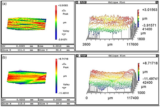
Figure 10.
Comparison of surface errors. (a) Estimating the alignment of the probe contact point to the nominal surface gives the same result. (b) Aligning the probe center point to the nominal surface by subtracting the probe radius gives incorrect results.
Finally, as another comparison, we also tested the probe radius compensated alignment method proposed by Xiong et al. [13]. This method involves subtracting the probe radius when calculating the point-to-surface distance for nominal surface alignment. However, experimental results (Figure 10b) showed that this method is not feasible, as it may lead to finding incorrect nearest points during the alignment process. This results in a decrease in alignment accuracy. Therefore, it is not appropriate to subtract the probe radius from the surface error obtained.
4. Conclusions
We propose a probe radius compensation and point cloud data alignment method specifically designed for solving significant alignment errors and discrepancies in high-steepness surfaces. In experiments, this method achieves a 3.95-fold reduction (from 27.3 μm to 6.9 μm) in PV face error and 78% reduction (from O(n3) to O(n)) in computational complexity compared to the traditional point-to-point method, based on the improved point-to-triangulation distance approximation. Furthermore, we propose an equidistant surface alignment method for compensating the probe radius, which enhances the robustness of the alignment algorithm, even for alignment errors as large as several 10 mm/°. We found that by optimizing the testing environment and inherent experimental errors, the above-mentioned PV face error may be closer to the simulation result of 10⁻⁶. In the future, this efficient point-to-triangulation point cloud registration method can be further combined with other intelligent algorithms, such as deep or reinforcement learning algorithm to adaptively optimize the meshing process, so as to accommodate more complex application scenarios. Finally, we believe that the algorithm we proposed can be used to guide compensatory machining to reduce surface shape errors in a low-cost, fast, and convenient manner, which is of great significance for the field of optical machining and measurement.
Author Contributions
Conceptualization, C.W., J.S., T.L., S.J. and L.L.; Methodology, C.W., H.H. and L.L.; Software, C.W.; Validation, C.W.; Formal analysis, C.W.; Investigation, C.W., F.C. and L.L.; Resources, C.W.; Data curation, C.W. and L.L.; Writing—original draft, C.W. and L.L.; Writing—review & editing, L.L. and C.Z.; Visualization, C.W.; Supervision, L.L. All authors have read and agreed to the published version of the manuscript.
Funding
This research was funded by National Natural Science Foundation of China, grant number 72071209, 51991371, 51835013, 52105567.
Institutional Review Board Statement
Not applicable.
Informed Consent Statement
Informed consent was obtained from all subjects involved in the study.
Data Availability Statement
Data available upon request.
Conflicts of Interest
The authors declare no conflicts of interest.
Abbreviations
| CMMs | Coordinate Measuring Machines |
| PV | Peak-to-Valley |
| RMS | Root Mean Square |
| IBF | Ion Beam Figuring |
| ICP | Iterative Closest Point |
| Minkowski Sum |
References
- Fang, F.; Zhang, X.; Weckenmann, A.; Zhang, G.; Evans, C. Manufacturing and measurement of freeform optics. CIRP Ann. 2013, 62, 823–846. [Google Scholar] [CrossRef]
- Yang, T.; Jin, G.-F.; Zhu, J. Automated design of freeform imaging systems. Light Sci. Appl. 2017, 6, e17081. [Google Scholar] [CrossRef] [PubMed]
- Peng, Y.; Dai, Y.; Song, C.; Shi, F. Tool deflection model and profile error control in helix path contour grinding. Int. J. Mach. Tools Manuf. 2016, 111, 1–8. [Google Scholar] [CrossRef]
- Dai, Y.; Chen, S.; Kang, N.; Li, S. Error calculation for corrective machining with allowance requirements. Int. J. Adv. Manuf. Technol. 2010, 49, 635–641. [Google Scholar] [CrossRef]
- Wang, X.; Xian, J.; Yang, Y.; Zhang, Y.; Fu, X.; Kang, M. Use of coordinate measuring machine to measure circular aperture complex optical surface. Measurement 2017, 100, 1–6. [Google Scholar] [CrossRef]
- Besl, P.J.; McKay, H.D. A method for registration of 3-D shapes. IEEE Trans. Pattern Anal. Mach. Intell. 1992, 14, 239–256. [Google Scholar] [CrossRef]
- Suh, S.-H.; Lee, S.-K.; Lee, J.-J. Compensating probe radius in free surface modelling with CMM: Simulation and experiment. Int. J. Prod. Res. 1996, 34, 507–523. [Google Scholar] [CrossRef]
- Lin, Y.C.; Sun, W.I. Probe radius compensated by the multi-cross product method in freeform surface measurement with touch trigger probe CMM. Int. J. Adv. Manuf. Technol. 2003, 21, 902–909. [Google Scholar] [CrossRef]
- Ravishankar, S.; Dutt, H.N.V.; Gurumoorthy, B. Automated inspection of aircraft parts using a modified ICP algorithm. Int. J. Adv. Manuf. Technol. 2010, 46, 227–236. [Google Scholar] [CrossRef]
- Song, C.-K.; Kim, S.-W. Reverse engineering: Autonomous digitization of free-formed surfaces on a CNC coordinate measuring machine. Int. J. Mach. Tools Manuf. 1997, 37, 1041–1051. [Google Scholar] [CrossRef]
- Chiang, Y.M.; Chen, F.L. Sculptured surface reconstruction from CMM measurement data by a software iterative approach. Int. J. Prod. Res. 1999, 37, 1679–1695. [Google Scholar] [CrossRef]
- Kawalec, A.; Magdziak, M. The selection of radius correction method in the case of coordinate measurements applicable for turbine blades. Precis. Eng. 2017, 49, 243–252. [Google Scholar] [CrossRef]
- Xiong, Z.; Li, Z. Probe radius compensation of workpiece localization. ASME J. Manuf. Sci. Eng. 2003, 125, 100–104. [Google Scholar] [CrossRef]
- Woźniak, A.; Mayer, J.R.R.; Bałaziński, M. Stylus tip envelop method: Corrected measured point determination in high definition coordinate metrology. Int. J. Adv. Manuf. Technol. 2009, 42, 505–514. [Google Scholar] [CrossRef]
- Wozniak, A.; Mayer, J.R.R. A robust method for probe tip radius correction in coordinate metrology. Meas. Sci. Technol. 2012, 23, 025001. [Google Scholar] [CrossRef]
- Chen, S.; Wu, C.; Xue, S.; Li, Z. Fast registration of 3D point clouds with offset surfaces in precision grinding of free-form surfaces. Int. J. Adv. Manuf. Technol. 2018, 97, 3595–3606. [Google Scholar] [CrossRef]
- Shimizu, Y.; Matsukuma, H.; Gao, W. Optical Sensors for Multi-Axis Angle and Displacement Measurement Using Grating Reflectors. Sensors 2019, 19, 5289. [Google Scholar] [CrossRef]
- Yuan, G.H.; Zheludev, N.I. Detecting nanometric displacements with optical ruler metrology. Science 2019, 364, 771–775. [Google Scholar] [CrossRef]
- Zhou, W.; Sun, Y.; Liu, Z.; Wang, W.; Liu, L.; Li, W. A Random Angle Error Interference Eliminating Method for Grating Interferometry Measurement Based on Symmetry Littrow Structure. Laser Photonics Rev. 2025, 19, 2401659. [Google Scholar] [CrossRef]
- Shimizu, Y.; Kanda, Y.; Ma, X.; Ikeda, K.; Matsukuma, H.; Nagaike, Y.; Hojo, M.; Tomita, K.; Gao, W. Measurement of the apex angle of a small prism by an oblique-incidence mode-locked femtosecond laser autocollimator. Precis. Eng. 2021, 67, 339–349. [Google Scholar] [CrossRef]
- Ruprecht, A.K.; Wiesendanger, T.F.; Tiziani, H.J. Chromatic confocal microscopy with a finite pinhole size. Opt. Lett. 2004, 29, 2130–2132. [Google Scholar] [CrossRef] [PubMed]
- Fan, C.; Xiao, C.; Xu, T.; Yu, D.; Chen, C.P. Decentralized event-trigger-based predefined-time adaptive control of large-scale nonlinear systems. J. Frankl. Inst. 2025, 362, 107446. [Google Scholar] [CrossRef]
- Ainsworth, I.; Ristic, M.; Brujic, D. CAD-based measurement path planning for free-form shapes using contact probes. Int. J. Adv. Manuf. Technol. 2000, 16, 23–31. [Google Scholar] [CrossRef]
- Li, S.; Dai, Y. Large and Middle-Scale Aperture Aspheric Surfaces: Lapping, Polishing and Measurement; John Wiley & Sons, Inc.: Hoboken, NJ, USA, 2017. [Google Scholar]
- Peng, Y.; Dai, Y.; Song, C.; Chen, S. Error analysis and compensation of line contact spherical grinding with cup-shaped wheel. Int. J. Adv. Manuf. Technol. 2015, 83, 293–299. [Google Scholar] [CrossRef]
Disclaimer/Publisher’s Note: The statements, opinions and data contained in all publications are solely those of the individual author(s) and contributor(s) and not of MDPI and/or the editor(s). MDPI and/or the editor(s) disclaim responsibility for any injury to people or property resulting from any ideas, methods, instructions or products referred to in the content. |
© 2025 by the authors. Licensee MDPI, Basel, Switzerland. This article is an open access article distributed under the terms and conditions of the Creative Commons Attribution (CC BY) license (https://creativecommons.org/licenses/by/4.0/).