Article

Detection of Vibration Signal by Plane Scanning Utilizing Wavefront Sensors

Key Laboratory of Vibration Signal Capture and Intelligent Processing, School of Electronic Engineering, Yili Normal University, 448 Jiefang Road, Yining 835000, China
*
Author to whom correspondence should be addressed.
These authors contributed equally to this work.
Photonics 2025, 12(4), 377; https://doi.org/10.3390/photonics12040377
Submission received: 13 February 2025 / Revised: 10 April 2025 / Accepted: 12 April 2025 / Published: 14 April 2025
(This article belongs to the Special Issue Editorial Board Members’ Collection Series: Photonics Sensors)

Abstract

:
Laser remote sensing of seismic waves is extensively utilized in earthquake monitoring and resource exploitation. This article leverages wavefront sensors’ high resolution and array detection capabilities to effectively conduct planar scanning of target areas in seismic wave laser remote sensing research, thereby properly acquiring regional vibration data. The error margin is between 1 % and 2 % relative to the source information.

1. Introduction

As the core means of resource exploration and environmental protection [1,2], seismic wave exploration technology can accurately identify key geological elements such as lithologic interface, fault structure, and fold shape by analyzing the coupling response characteristics of elastic wave field and geological medium and provide quantitative geophysical parameters such as wave impedance inversion and seismic data quantitative interpretation technology for mineral resource assessment [3,4,5,6]. Through travel time tomography and a full waveform inversion algorithm [7], this technology can build a three-dimensional velocity structure model and realize the three-dimensional characterization of oil and gas storage spatial distribution and physical parameters [8]. However, the traditional seismic exploration has significant exploration blind areas in high altitude no man’s land and complex structural zones. At present, it is urgent to develop the aerial seismic wave laser remote sensing system to achieve large-scale, high-resolution seismic field aerial monitoring.
In recent years, seismic wave laser remote sensing technology has rapidly developed, using high-resolution [9], non-contact laser measurements to accurately analyze seismic waveforms, identify geological structures [10,11], and evaluate the distribution of minerals, oil, and natural gas [12,13]. Compared to traditional methods, this technology can detect weak vibrations from a distance [14,15], breaking through the limitations of complex terrain and deep exploration. Combining remote sensing [16], GIS [17], and satellite data [18], laser remote sensing has improved exploration efficiency and accuracy, identified resource potential areas at lower costs, and promoted deep geological research and energy development.
Laser remote sensing detection technology has the advantages of non-contact measurement, fewer restrictions, higher efficiency and long-distance detection, and is widely used in object vibration detection. In order to meet the challenges of long-range laser echo signal attenuation and vibration waveform analysis, researchers have explored the use of the He-Ne laser interferometer [19] and Michelson interferometer [20] to measure vibration signals. However, these technologies depend on the complex optical system and the setting of the reference arm and the measurement arm, which has certain limitations. Therefore, Silvio Bianchi [21] proposed a new method without using an interferometer to sense the surface vibration signal by using the speckle pattern formed after laser irradiating the rough surface. This method can effectively detect the vibration signal within a distance of several hundred meters. There are many methods to detect ground vibration signal based on phase, such as wavefront sensor [22,23,24], shear interference [25,26], and so on. Jorge ares et al. [27] used the Shack–Hartmann wavefront sensor as a position sensing device to accurately determine the position of a point or moderately extended plane object.
Compared to traditional seismic wave laser remote sensing technology, wavefront sensors have significant advantages in detecting ground vibrations. Firstly, it eliminates the need for reference arms and measurement arms, making the device more compact and easy to deploy. Secondly, by measuring the phase change of the wavefront, precise mechanical vibration information can be obtained. In addition, wavefront sensors have array detection capabilities, which improve detection accuracy and application range. In 2023, researchers constructed a seismic wave laser remote sensing system based on wavefront sensors [28] and successfully detected ground vibration signals [29]. However, existing methods mainly collect single point vibration information, which makes it difficult to process regional vibration signals and has limited detection efficiency. Therefore, based on the research in reference [28], this article proposes a region vibration detection method based on laser plane scanning, utilizing the array detection characteristics of wavefront sensors, to achieve high-precision and high-resolution vibration measurement.

2. Vibration Signal Laser Plane Scanning Detection System and Its Operational Mechanism

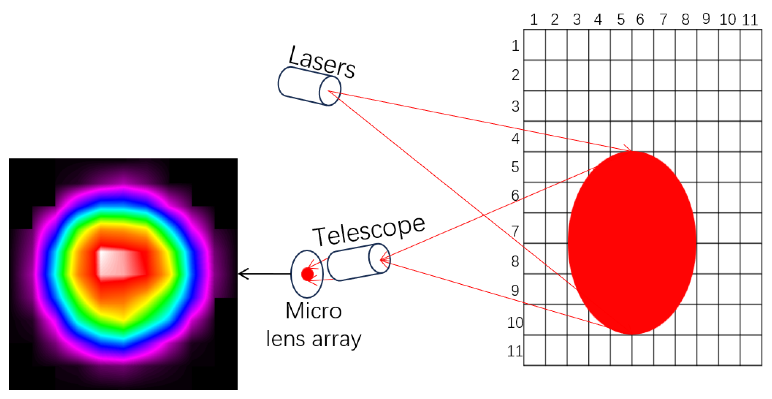
When an earthquake occurs, longitudinal waves cause vertical ground vibrations, which, in turn, change the wavefront of the incident light, causing the backscattered light of the laser to carry the characteristic information of seismic waves. In wavefront measurement systems, laser irradiates the target area in a vertical or oblique manner, and the small fluctuations on the measured surface cause light scattering and reflection. Subsequently, the micro lens array converges and images these reflected or scattered light, and extracts vibration information through wavefront reconstruction to achieve accurate measurement of seismic wave characteristics.
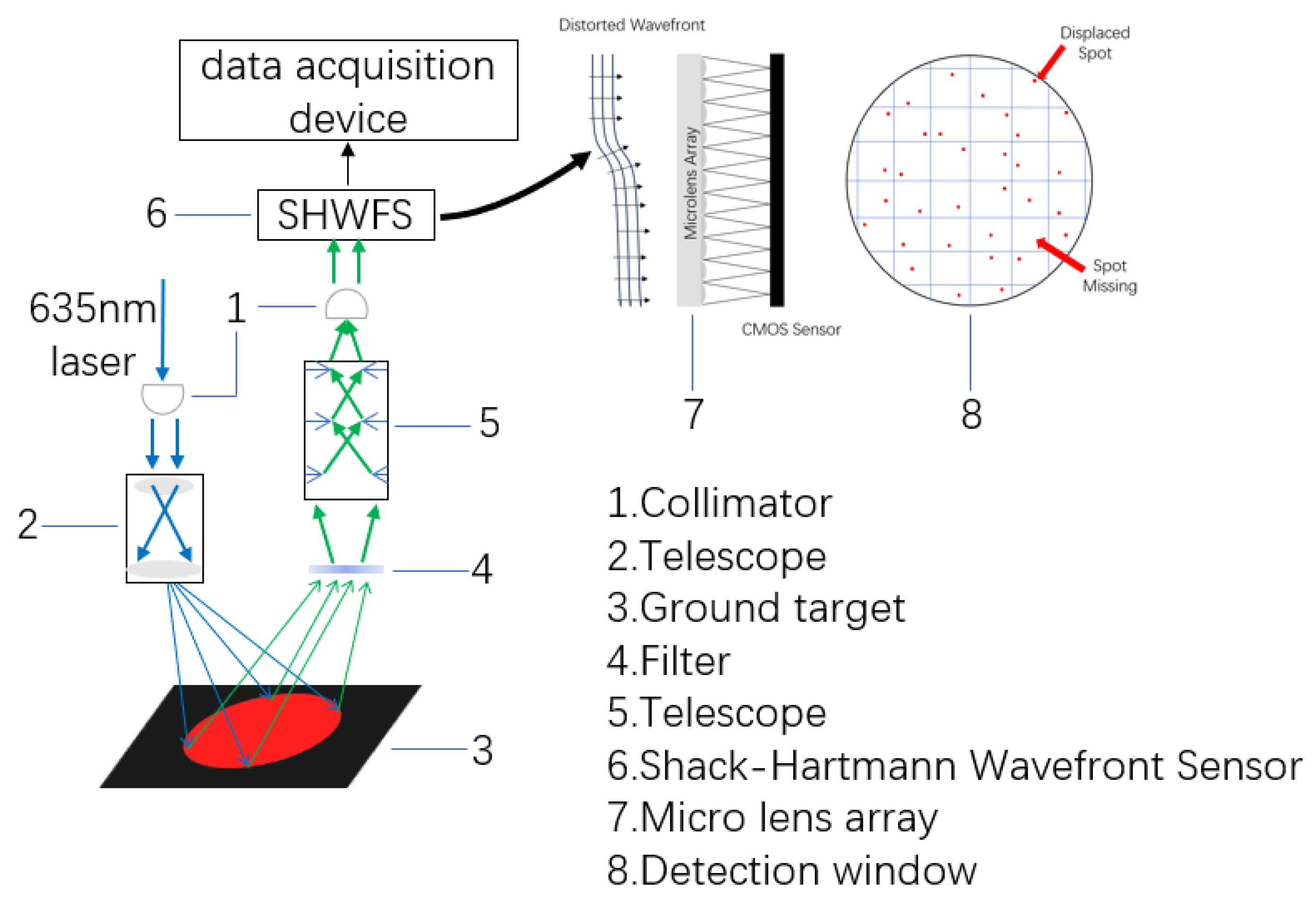
This article proposes a vibration signal remote sensing detection system based on planar scanning that consists of a transmitting end and a receiving end, as shown in Figure 1. The transmitting end includes a laser, collimator 1, and telescope 2. The system uses a gradient refractive index fiber collimator to emit a laser beam with a divergence angle of 0.25°, and its oxide glass material collimating lens achieves collimated output with a beam quality factor M2 < 1.1 through a 0.15 numerical aperture. The laser emits a continuous laser with a wavelength of 635 nm and is collimated by a tail fiber type fiber collimator 1 (equipped with a gradient refractive index GRIN lens) to ensure stable illumination of the target area 3. The receiving end consists of telescope 5, filter 4, and wavefront sensor 6. This is a bandpass filter that can filter out 97% of stray light within the wavelength range of 624–750 nm. The telescope is responsible for collecting reflected and scattered light from target area 3, while filter 4 is used to remove stray light from the environment to improve the utilization of echo signals. Subsequently, the light passing through the filter is incident on the wavefront sensor 6, which is composed of a micro lens array 7 and can accurately detect wavefront distortion in the optical system. The micro lens array divides the incident light spot into multiple sub apertures and focuses the imaging onto the light spot detection window 8 in the array. The system extracts vibration information by measuring the offset of the light spot and uses laser remote sensing technology to detect micro vibrations in the target area. We study the relationship between the phase information of the target vibration and the offset of the received light spot on the CMOS sensor. When the target object 3 vibrates, the displacement Δ S of the center of mass of the light spot recorded by the wavefront sensor carries vibration information Δ Z . According to reference [28], the relationship between the two satisfies the equation Δ Z = μ Δ S , where μ is the proportionality coefficient. 
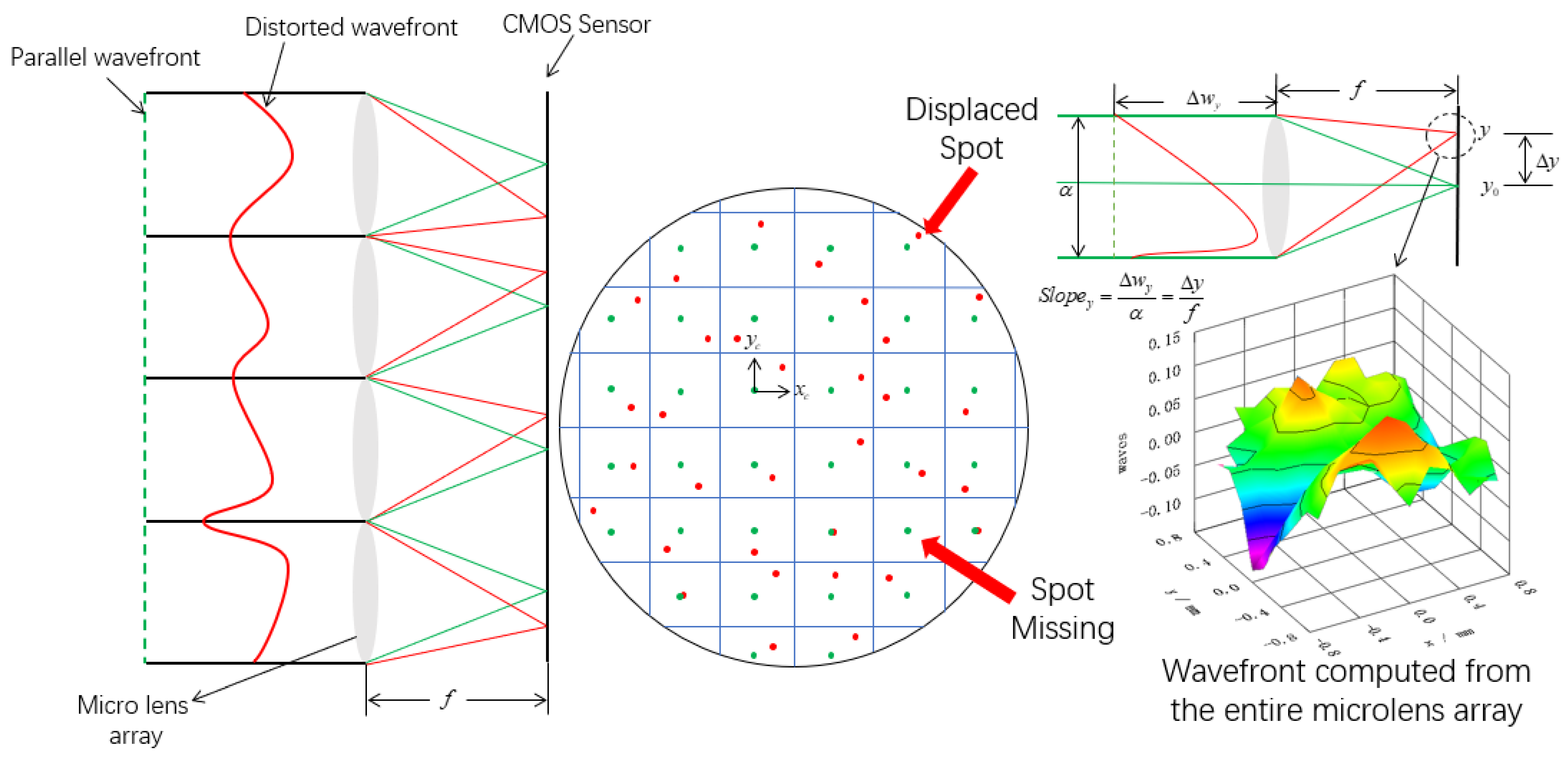
Figure 2 shows the changes in wavefront during the vibration process. In Figure 2, we simplify the analysis by assuming the ground is flat when not vibrating. This assumption is made to illustrate the basic relationship between the transmitted and reflected wavefronts. In reality, uneven ground may combine with other non-ideal factors to influence the wavefront’s shape.
In an ideal situation, when a parallel wavefront is irradiated onto a micro lens array, each micro lens will focus the incident light, forming a uniformly distributed light spot, and the centroid position of these light spots should be located at the predetermined center position. Therefore, the distribution of light spots formed by the micro lens array is regular and symmetrical, with each light spot representing a local area of the wavefront, reflecting the degree of wavefront tilt in that area. However, when the wavefront undergoes distortion, the incident light no longer maintains a parallel state, and local areas of the wavefront become tilted or deformed. At this point, the micro lens array will convert these wavefront changes into corresponding spot offsets. The difference between the centroid shift of the light spot caused by distorted wavefront and the ideal position can be used to quantify the degree of wavefront distortion, as shown in Figure 3.

3. Theoretical Analysis of Vibration Signal Laser Plane Scanning Detection System

3.1. Wavefront Reconstruction Using Zonal Methods

This article adopts the region method proposed in references [30,31,32,33,34] for wavefront reconstruction. We used the wavefront slope S corresponding to the vibration wavefront shown in Figure 2 for reconstruction and successfully obtained the corresponding wavefront distribution, as shown in Figure 4.

3.2. Wavefront Phase

To calculate the phase from the reconstructed wavefront, the following formula can be used [35]:
Δ φ = 2 π λ | Δ W |
Here, φ ( x , y ) is the phase, W ( x , y ) ; and λ is the wavelength. Therefore, the phase change of the wavefront was obtained using the wavefront in Figure 4, as shown in Figure 5. Wavefront sensors can capture wavefront distortion caused by vibration and derive amplitude changes by measuring changes in wavefront phase. When using Shack–Hartmann sensors, the micro lens array records the slope changes in various directions and then calculates the phase distortion of the wavefront. By analyzing the phase change of the wavefront sensor during vibration, the relationship between amplitude and phase can be established, and the formula is as follows:
Δ φ = k Δ d + c
Here, Δ φ represents phase change, and Δ d is the amplitude variation. In the absence of vibration, the laser echo received by the wavefront sensor will cause a slight shift in the centroid of the light spot on the micro lens array, resulting in a slight change in the wavefront slope. The constant term c in the formula reflects this shift.
This article uses the region method to reconstruct the wavefront of a certain region, obtaining a global wavefront. However, it is impossible to obtain each microlens’ wavefront contribution directly. To solve this problem, we separate the overall wavefront and remove the PSF connections between each microlens, thereby obtaining the wavefront phase changes of each microlens during vibration. Through this method, the vibration situation of each subregion can be visually observed, as shown in Figure 6. This method effectively separates and analyzes the vibration characteristics of each subregion, revealing the spatial distribution and variation patterns of vibration.

3.3. Laser Attenuation

A laser has geometric attenuation and atmospheric attenuation in atmospheric transmission [36,37]. As the propagation distance of the laser beam increases, its light intensity gradually decreases due to the expansion of the beam. Geometric attenuation describes the decrease in laser intensity during propagation due to the expansion of the beam. At the propagation distance z, the beam’s diameter increases with distance, resulting in a decrease in light intensity per unit area. Assuming the divergence angle of the beam is θ , the diameter d ( z ) and area A ( z ) of the light spot at the propagation distance z is
w ( θ ) = z t a n ( θ )
d ( z ) = 2 z t a n ( θ )
A ( z ) = π [ d ( z ) 2 ] 2 = π z 2 t a n 2 ( θ )
As the propagation distance of the laser beam increases, its light intensity gradually decreases due to the expansion of the beam. Assuming the initial light intensity of the laser, since the light intensity is inversely proportional to the area, the geometric attenuation can be expressed as
I g e o z = k I 0 w 2 z e x p 2 r 2 w 2 z
Among them, k is a constant, and w ( z ) is the beam’s radius. When a laser passes through the atmosphere, it is also subject to scattering and absorption by the atmosphere, resulting in a decrease in light intensity. Assuming the absorption and scattering coefficients of the atmosphere are α , the effect of atmospheric attenuation can be described by the following formula:
I a t m z = I 0 e α z
When there are both geometric and atmospheric attenuation, light intensity attenuation is the combined effect of both. Assuming the initial light intensity, we can combine the attenuation models of both to obtain the overall attenuation formula:
I z = I g e o z I a t m z
Substitute the above two formulas into
I z = I 0 e α z k I 0 w 2 z e x p 2 r 2 w 2 z
Therefore, the overall light intensity attenuation model is
I z = k I 0 2 e α z w 2 z e x p 2 r 2 w 2 z
Here, I 0 is the initial light intensity, z is the propagation distance, θ is the divergence angle of the laser, and α is the atmospheric attenuation coefficient.

4. Experimental and Result Analysis of the Vibration Signal Laser Plane Scanning Detection System

We use a laser with a wavelength of 635 nm and an output power of 120 mW at a distance of 5 m. In order to reduce the interference of ambient light and increase the reception effect of the laser echo signal of the wavefront sensor, we choose to carry out the experiment at night. The temperature of the laboratory is 14 ℃, the humidity is 23%, and the change in the surrounding environment is very small. 
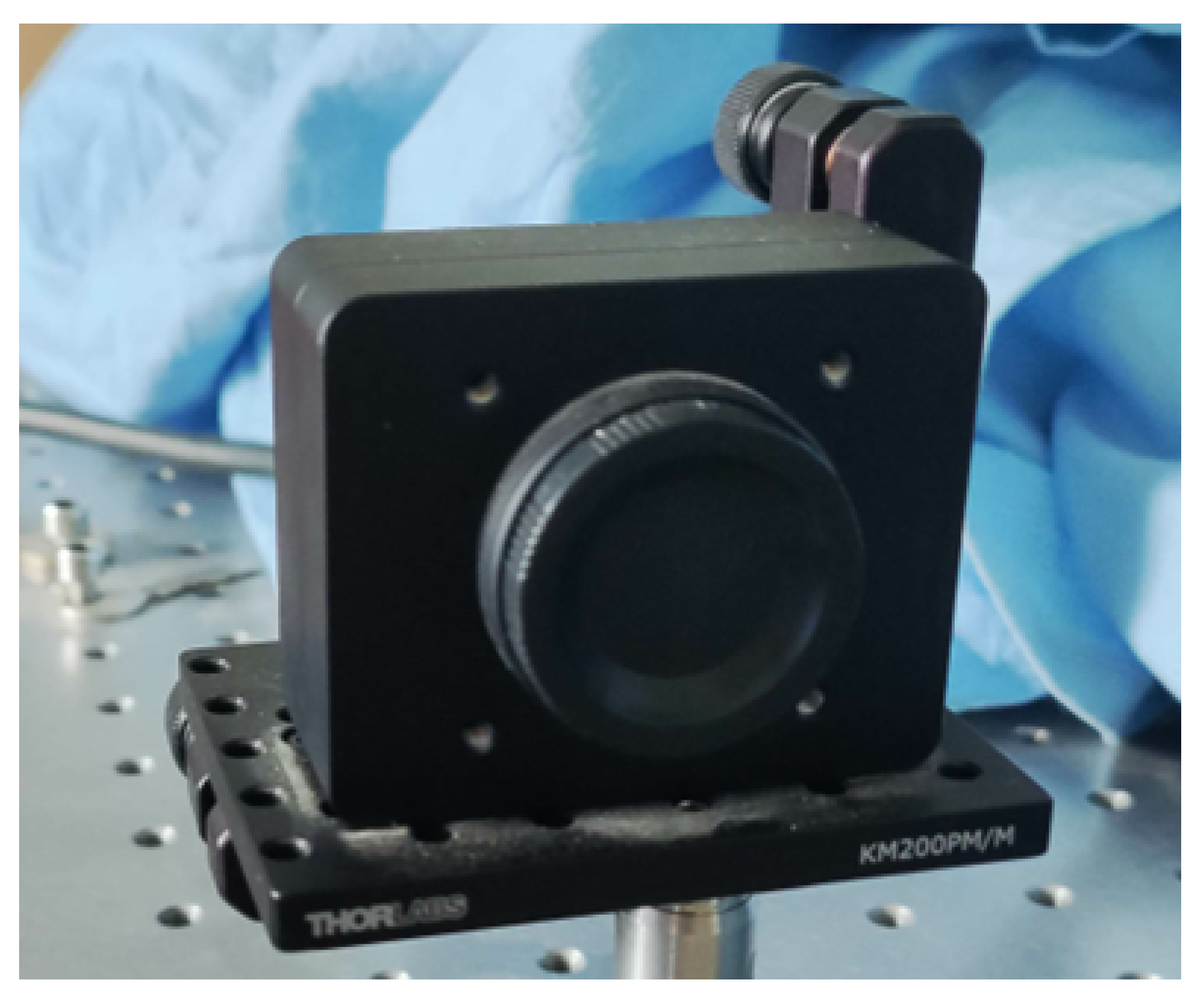
Figure 7 shows the sensor used for research, and 
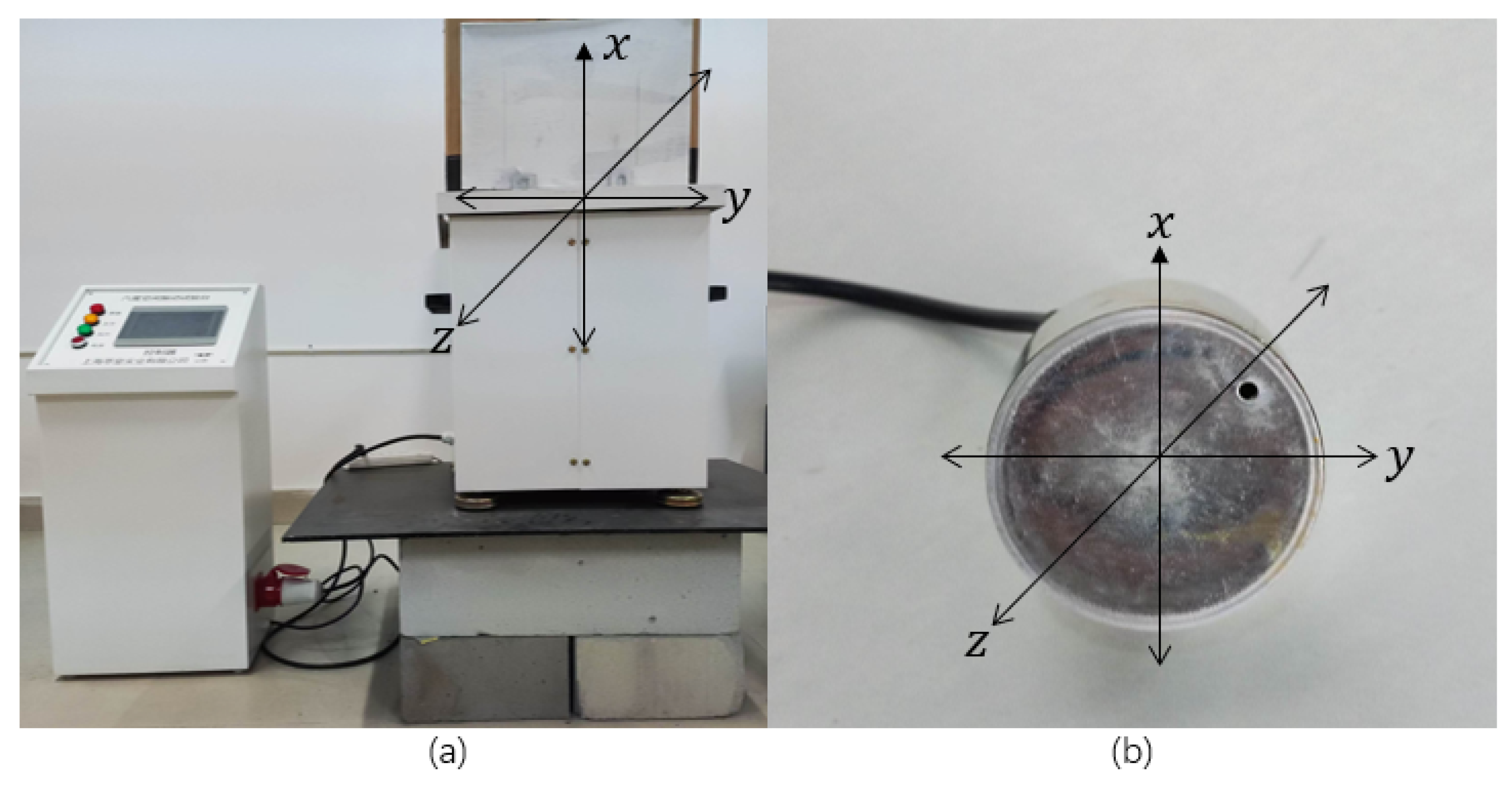
Table 1 shows the detailed parameters of this model of sensor. The sensor has high sampling rate and automatic shutter control function, which can adapt to different optical power inputs, and its sensitivity is significantly affected by wavelength, making it suitable for detecting ground vibration signals. In the single point detection experiment, we used a controllable vibration table to simulate longitudinal wave characteristics by adjusting frequency and amplitude, Figure 8a shows a diagram of a controllable vibration table; In the surface scanning experiment, a vibration motor is used as the vibration source, and the interference of the vibration source is isolated by a soft white cloth. Figure 8b shows a diagram of vibration motor. The laser irradiates the surface of the vibration source, and the wavefront sensor receives the reflected echo light and extracts vibration information. To monitor the wavefront changes of the wavefront sensor in real time, we use Wavefront Sensor software to record the wavefront dynamics and use LabView software to calculate and display the changes in individual microlenses in order to deeply analyze the response of the wavefront when excited by the vibration source. The specific program flow is detailed in Appendix A. The system configuration and data recording method ensure accurate monitoring and analysis of small wavefront changes caused by vibration sources. Figure 9a shows the deviation in wavefront slope in the horizontal and vertical directions when the vibration source vibrates. When longitudinal waves are detected, the deviation in the y direction is larger, while the deviation in the x direction is smaller. Meanwhile, Figure 9b shows the vibration signal recorded using a vibrometer.
When testing the light spot received by a single microlens, the laser echo signal is focused onto a certain microlens in the microlens array through a telescope. In the beam view mode of the wavefront sensor, in addition to the target microlens, several adjacent microlenses around it will also display weak spot signals, as illustrated in Figure 10. This indicates that the relationship between laser echo signals and microlens arrays is not simply “one-to-one” but presents more complex “one to many” characteristics.
We tested the attenuation of laser power, and this effect usually shows a certain pattern. We used a 635 nm continuous laser to irradiate the target area separately and measured the laser power using an optical power meter, as shown in Table 2. The test results indicate that the laser power shows an exponential decay trend with increasing irradiation distance. Table 2 is only applicable for small-scale laboratory testing. When the receiving end is a wavefront sensor, the attenuation of laser power will significantly affect the accuracy of surface scanning detection, which is reflected in the reduction in signal amplitude, which leads to the reduction in the contrast and signal-to-noise ratio of the wavefront speckle pattern received by the detector, resulting in the inaccurate estimation of speckle location error and wavefront gradient and further causing the accumulation of wavefront reconstruction error; especially when the sub aperture signal is too weak or missing, local wavefront information will be missing or distorted. In addition, the nonuniformity of energy attenuation in spatial distribution will also destroy the spatial response consistency of the system, which will reduce the geometric reconstruction accuracy of the whole surface scanning, especially in the long distance, edge area or weak reflection surface.
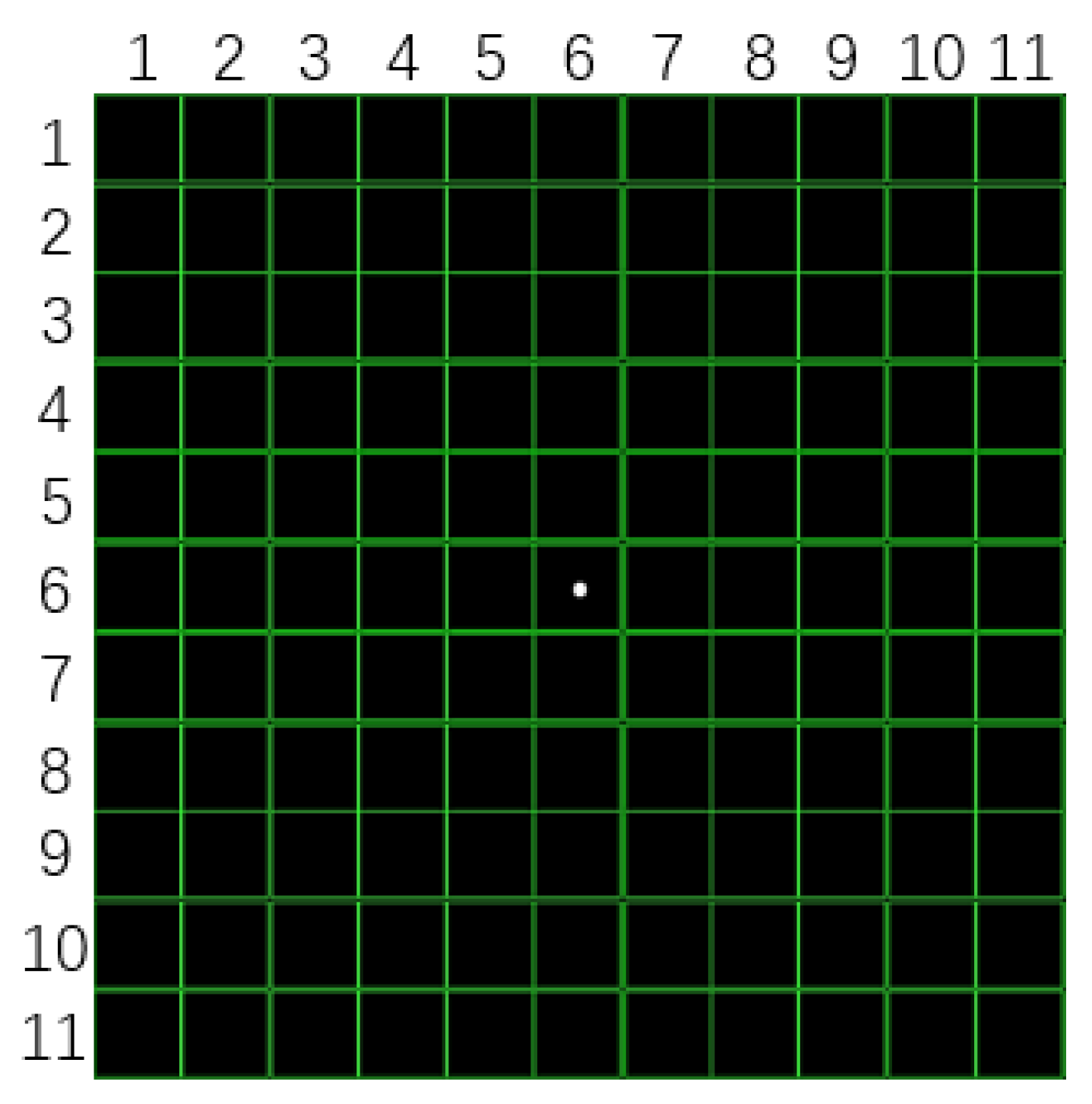
We mark the 11 × 11 microlenses of the wavefront sensor as 1 × 1 coordinates from the upper left corner, as shown in Figure 11. The laser forms a spot surface on the shaking table, and the echo signal is focused on the microlens with the coordinates of 6 × 6 of the wavefront sensor through the telescope. The wavefront slope and wavefront images of the microlens with coordinates of 6 × 6 
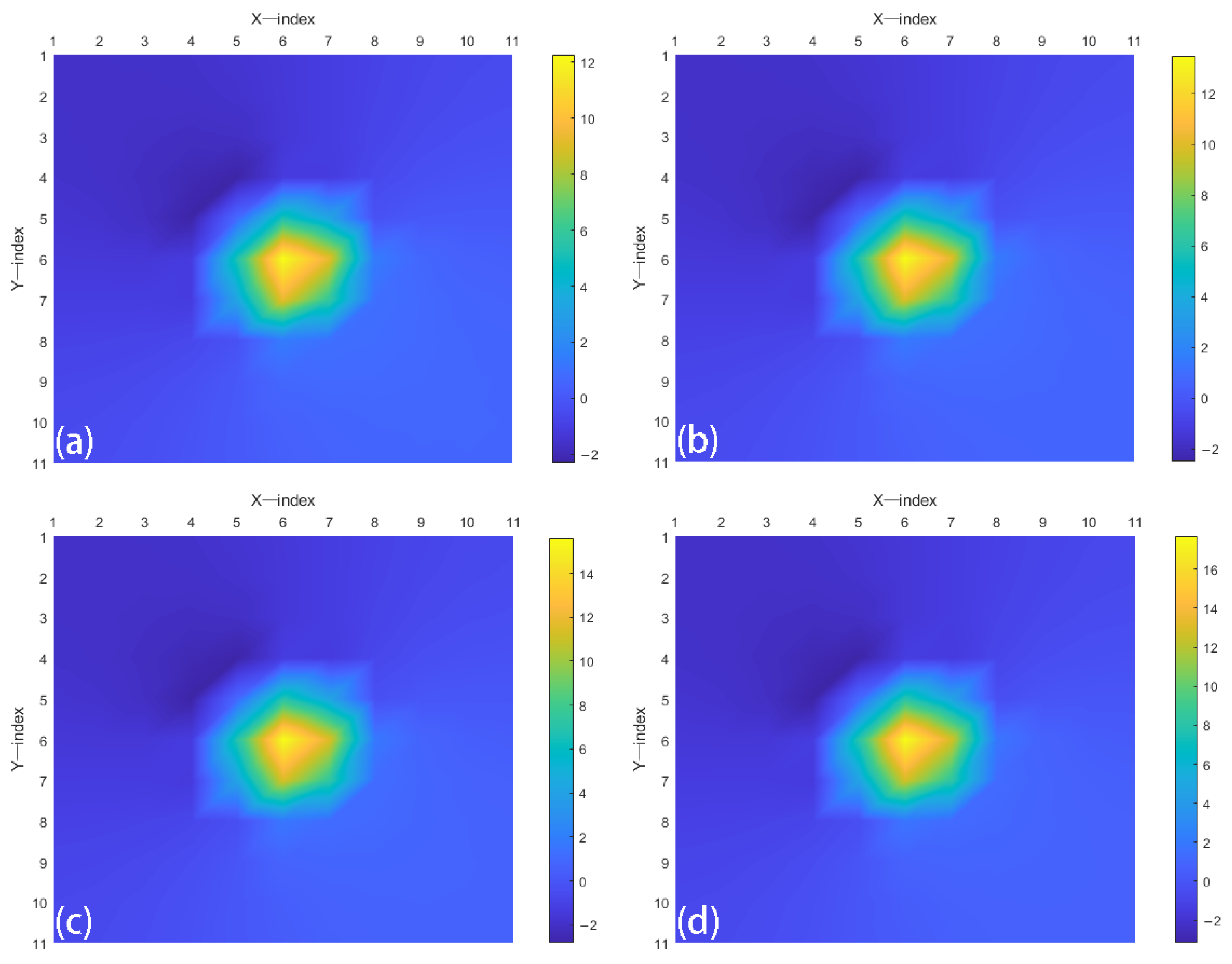
and adjacent microlenses were obtained by using LabVIEW software, and the corresponding wavefront images were reconstructed by using the region method. As shown in Figure 12, with the increase in vibration amplitude, the degree of wavefront distortion increases accordingly, and the microlens around the microlens with coordinates of 6 × 6 is also slightly disturbed. Changes in amplitude and wavefront phase are shown in 
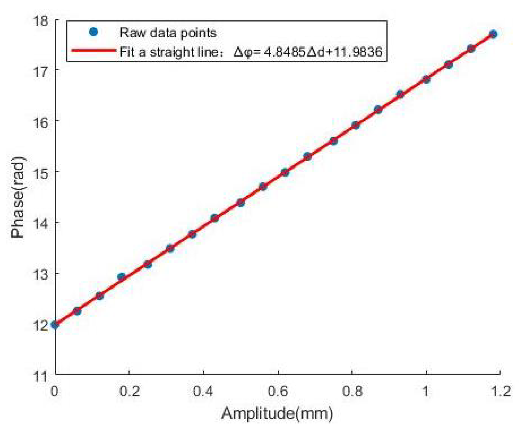
Appendix B. When there are vibration signals with different amplitudes in a certain area, the laser echo signal will carry the vibration information of the area. By receiving these laser echo signals, the wavefront sensor obtains and analyzes the corresponding vibration information. By analyzing the wavefront phase changes under different amplitudes, the relationship between amplitude and phase can be revealed, as shown in Figure 13. The wavefront phase shifts with the change in amplitude, which makes it possible to deduce the variation law of amplitude by measuring the phase change, as shown in the following formula:
Δ φ = k Δ d + c , k = 4.8485 mm / rad , c = 11.9836
Based on the above experiment, we divided a 1.2 m × 1.2 m target object into 11 × 11 sub regions, starting from the upper left corner, with the first region marked as 1 × 1 coordinate, and established an array in order. We randomly arranged multiple vibration sources within the 11 × 11 sub regions of the target object. We perform planar scanning on each subregion to obtain the corresponding changes in the wavefront slope of the microlens, as seen in Figure 14. A one meter diameter light spot is formed on the target area, and the laser echo signal is focused onto a microlens array through a telescope. Thirty-two microlenses in the microlens array receive the signal. In the target area, there are 4 sub areas with very small spot signals that cannot cover most of their area. Therefore, there are 4 microlenses in the microlens array that have no signal. We extract the changes in wavefront slope during the vibration of 32 microlenses and reconstruct the corresponding wavefront phase changes for each subregion. We calculate the corresponding vibration amplitude based on the wavefront phase changes in each subregion.Therefore, only one system is needed to obtain vibration information of multiple sub regions within the target area. 
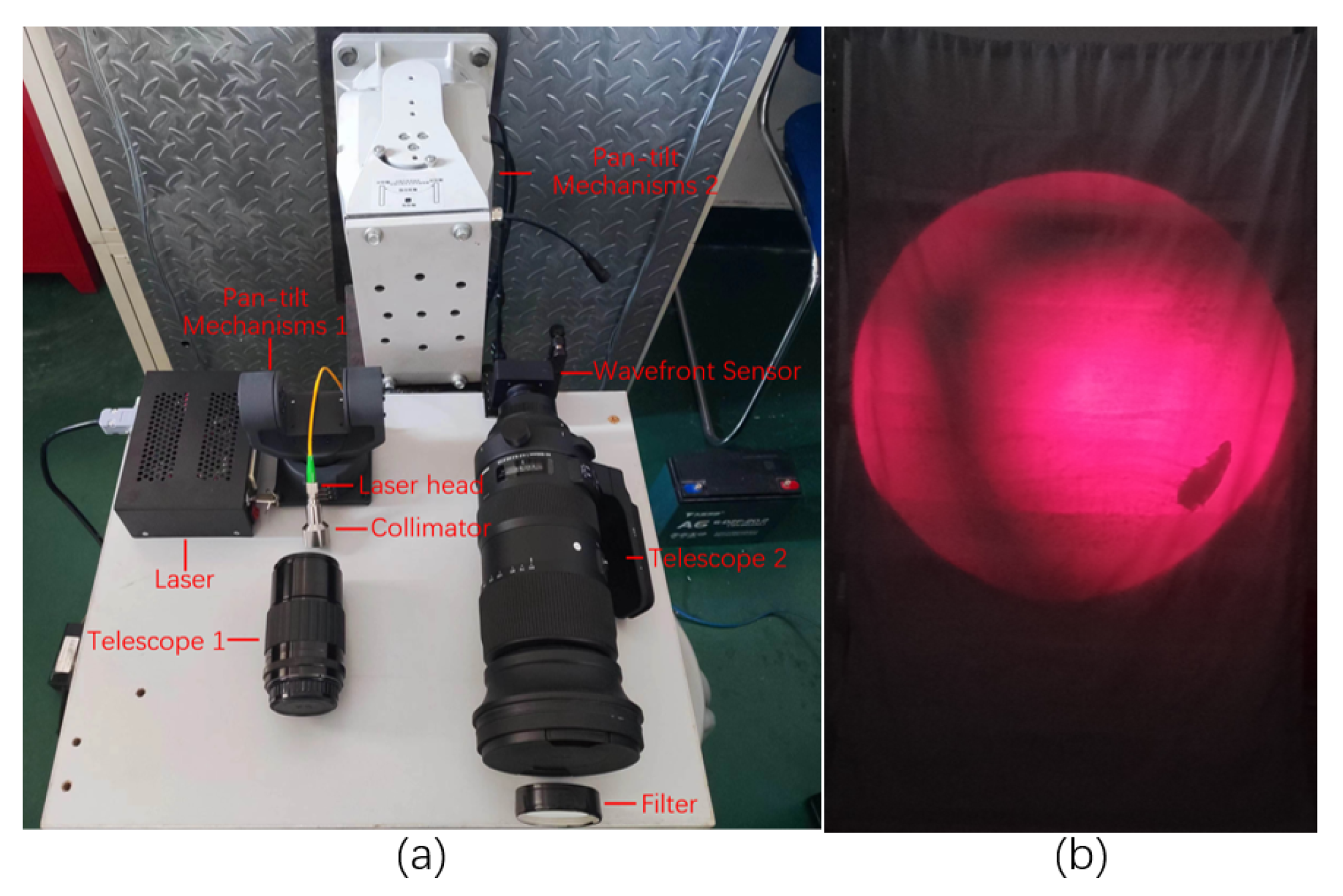
Figure 15 shows the physical device of the object and the 1 m light spot formed in the target area. The field of view of the telescope is 4 . 1 39 . 6 , and the distance between the telescope and the spot is 5 m. Therefore, the 100 cm spot size is fully within the field of view of the telescope. During the detection process, we first use pan-tilt 1 to project the collimated laser onto the target area. Then, we use a clamp to fix telescope 1 and manually adjust its objective lens and eyepiece to adjust the spot area on the target area. Then, we use pan-tilt 2 to adjust the receiving angle of telescope 2 and further adjust the objective lens and eyepiece of telescope 2 to ensure the best receiving effect. Subsequently, through the high-speed sampling interface of the wavefront sensor, we manually adjust the position of the wavefront sensor so that the laser echo signal can be accurately focused on the corresponding lens in the wavefront sensor microlens array, thereby achieving vibration signal point scanning detection. The spatial resolution of the system in Figure 15a is 146 μm.
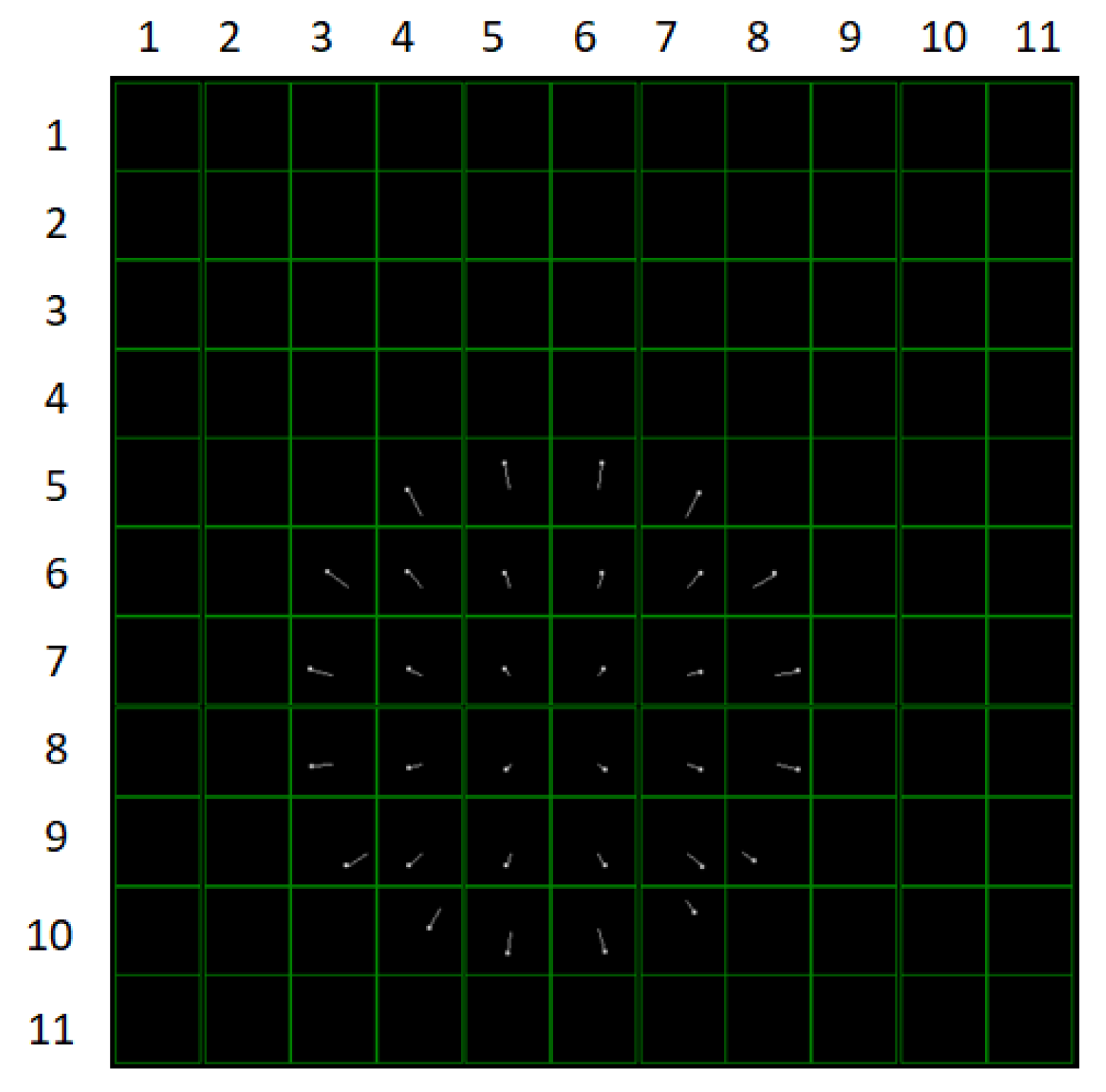
We divide the 1.2 m × 1.2 m target area into 11 × 11 sub areas; divide the target area into four areas, each including 36 sub areas of the target area; and place vibration sources within the 36 sub areas. Using a telescope, a laser beam is directed onto the target object to form a spot with a diameter of 60 cm, while detecting 36 sub regions within the target area. However, due to the shape of the spot, only 32 subregions can actually be detected. The laser echo signal is focused by a telescope and forms a spot surface on the microlens array of the wavefront sensor. In the high-speed sampling mode of the wavefront sensor, the 32 microlenses of the microlens array received laser echo signals within the target area, as shown in Figure 16. Subsequently, the LabView software was used to accurately locate the microlenses in the array that correspond to the target subregion, thereby obtaining the wavefront slope changes in the corresponding microlenses and calculating the corresponding wavefront phase. As shown in Figure 16, due to the inconsistent vibration amplitudes in the 32 sub regions of the target area, the wavefront slope of each sub region in the 32 sub regions is different.
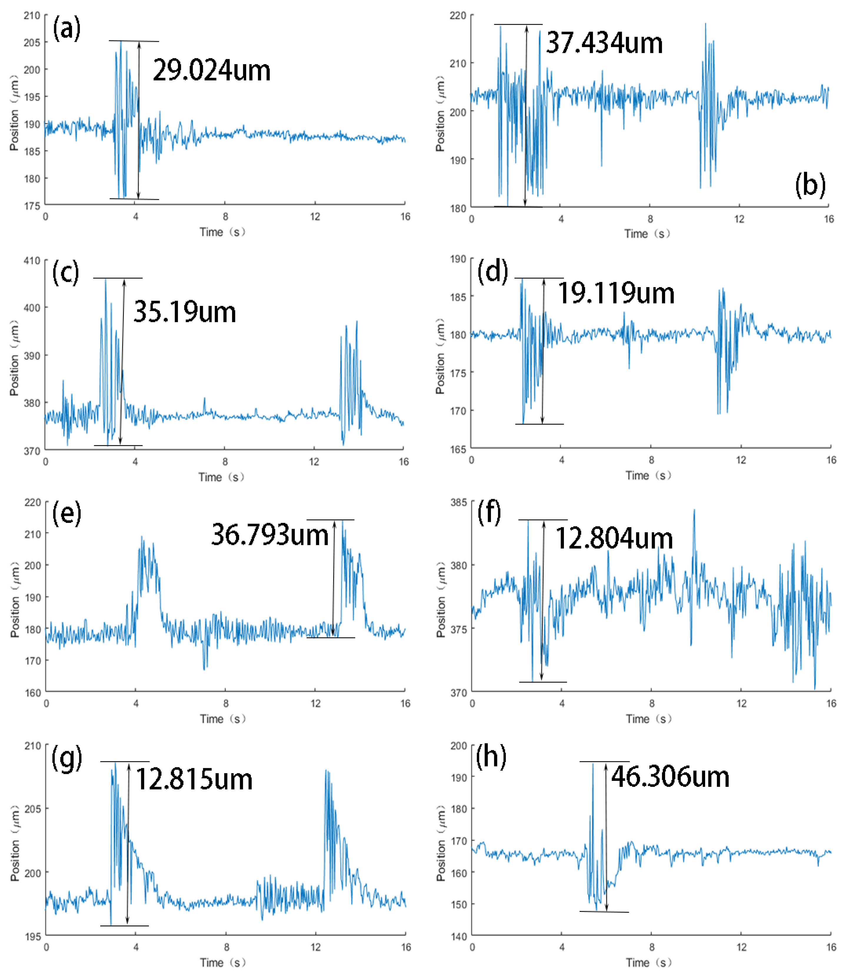
We sample a region multiple times. We selected 8 microlens spot centroid changes from Figure 16, as shown in Figure 17. Figure 17 shows the centroid displacement of the light spot in eight sub regions of the target area. The vibration amplitudes of different subregions in the target area are inconsistent, and the vibration amplitudes displayed on the microlens array of the wavefront sensor are also inconsistent. Due to the use of a vibration motor, the orientation of the echo laser received by the wavefront sensor will undergo a slight change, and the center of mass of the illuminated spot will continue to move. As shown in Table 3, the offset of the center of mass of each microlens in the microlens array is different due to the inconsistent amplitude of the target subregion.
According to the detection in the vicinity of Figure 16, the target area of 1.2 m × 1.2 m is partitioned into 11 × 11 sub-regions, placing all sub areas in the target area with vibration sources. The whole target area is divided into a 4 × 4 area, and each area is detected by plane scanning. Utilizing a telescope, the laser beam creates a spot with a diameter of 60 cm on the target area, concurrently identifying the 32 sub-regions within that area. The telescope concentrates the laser echo signal, creating a light spot on the microlens array of the wavefront sensor. Thereafter, the microlens associated with the designated sub-region in the microlens array is accurately identified using LabView software, facilitating the acquisition of the wavefront slope variation of the respective microlens and the computation of the related wavefront phase, as illustrated in Figure 18. Figure 18 illustrates that variations in the magnitude of the vibration source correspondingly alter the wavefront phase. This signifies that the vibration signal laser planar scanning detection system can efficiently identify the vibrational states of several small locations inside the designated zone. The calculated vibration amplitude via phase changes exhibits a relative inaccuracy of 1 % to 2 % compared to the amplitude recorded by the vibration meter, as illustrated in Figure 19.
In order to improve scanning efficiency, we further expanded the spot area. Similarly, a circular spot with a diameter of 1 m can only cover 69 sub areas of the target area. The 1.2 m × 1.2 m target area is divided into 11 × 11 sub areas, and 69 sub areas are selected to place vibration sources. The laser beam uses a telescope to form a spot with a diameter of 1 m on the target area and covers 69 sub areas in the target area. The laser echo signal is focused on the microlens array through the telescope, and 69 microlenses on the microlens array receive the signal, as shown in Figure 20. We use LabVIEW software to obtain the wavefront slope of 69 microlenses and calculate the wavefront phase change of each microlens so as to obtain the amplitude of the corresponding sub region in the target region. At present, the detection of a 1.2 m × 1.2 m target area is only achieved in a relatively stable laboratory environment. Due to the lack of high-power lasers and telescopes with large viewing angles, it is temporarily impossible to achieve large-scale scanning.
The telescope concentrates the laser echo signal, creating a light spot on the microlens array of the wavefront sensor. LabView software is used to precisely identify the microlens associated with the designated sub-area and acquire the phase variation of the vibrating wavefront through the alterations in wavefront slope induced by vibration. This enables the prediction of amplitude values based on the phase change. 
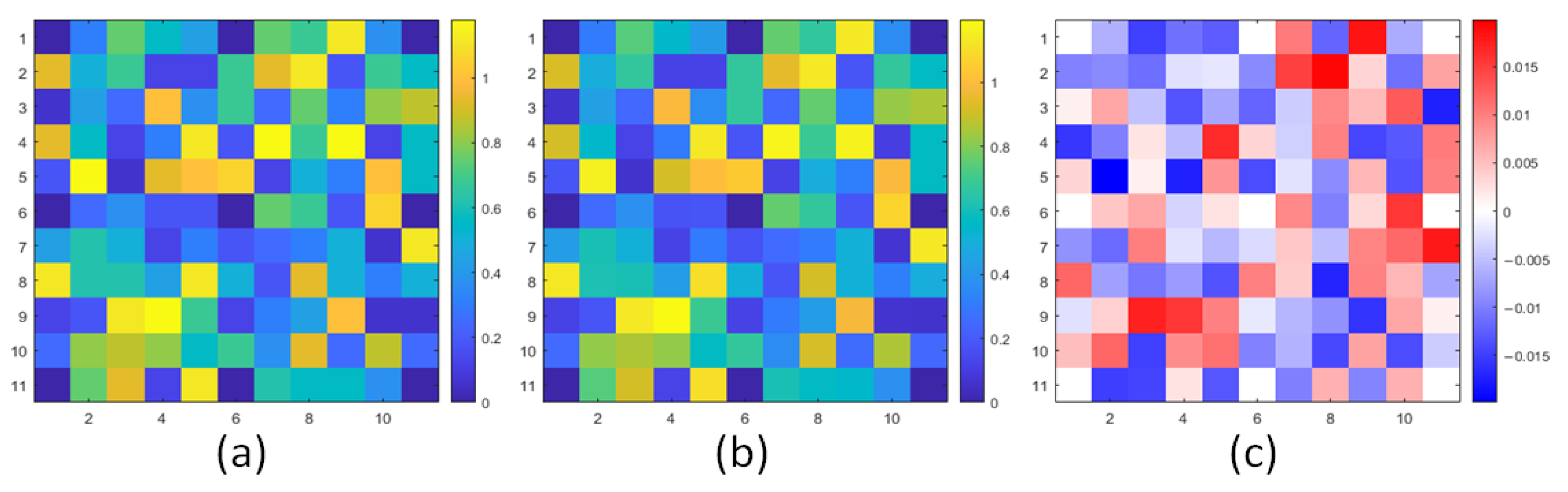
Figure 21 illustrates the outcomes of identifying a region with three vibration sources utilizing a 69 microlens, exhibiting a relative inaccuracy of 1 % to 2 % .
This research employs the zonal approach for wavefront reconstruction of a specified region, deriving the wavefront distortion associated with the microlenses of each sub-region and facilitating an intuitive analysis of the vibrational conditions of each sub-region, as illustrated in Figure 21. This method enables the effective separation and analysis of the vibration characteristics of each sub-region, elucidating the spatial distribution and variation patterns in the vibrations. In the experiment, we initially process the wavefront data obtained from the wavefront sensor, employing the zonal approach to divide them into several sub-regions. By reconstructing the wavefront of each sub-region, we can achieve higher-resolution vibration images, which are essential for recognizing local vibration sources and comprehending vibration transmission mechanisms.
This article is based on the characteristics of high resolution and sensitivity of wavefront sensors to detect low-frequency vibration signals, as shown in Figure 22. As shown in Figure 22, as the frequency of the controllable vibration table gradually increases, the frequency of the detected signal also increases.
We conducted tests on the maximum and minimum vibration amplitudes using a controllable vibration table. The vibration frequency of the vibration table was set to 0.1 Hz, and the wavefront sensor was set to high-speed sampling mode (sampling rate: 700–880 fps). Therefore, this paper achieved the detection of large amplitude vibration with a vibration amplitude of 5.94 mm and small amplitude vibration with a vibration amplitude of 0.06 mm, as shown in Figure 23. However, due to the insufficient sampling rate of the wavefront sensor, it is unable to detect high-frequency vibration signals.
The detection accuracy has been markedly enhanced relative to the conventional laser triangulation approach by utilizing minor wavefront alterations to identify a specific area’s vibrational signals. The error in detection by wavefront distortion ranges from 1.06 % to 2 % , but the error in detection utilizing the laser triangulation method spans from 1.54 % to 3.5 % , as illustrated in Table 4. Wavefront sensors can accurately detect phase alterations in light waves, enabling more sensitive assessments of minute vibrations. In contrast to the laser triangulation method, which depends on variations in the light spot’s position, wavefront sensors can efficiently mitigate environmental noise and external disturbances by examining the comprehensive phase information of the light wave, thereby yielding more stable and dependable vibration monitoring outcomes. Moreover, wavefront sensors possess benefits in spatial resolution, facilitating high-density sampling across extensive areas, hence, rendering vibration analysis more thorough and intricate.
Although the seismic wave laser remote sensing surface scanning method based on the wavefront sensor shows good application prospects in laboratory conditions, it still faces many challenges in the actual environment. Atmospheric turbulence will cause the phase distortion of the laser wavefront, interfere with the measurement accuracy, and its influence fluctuates significantly with the change in altitude, time, and meteorological conditions. In addition, aerosols such as dust and haze will aggravate the scattering and attenuation of laser signals. Uneven distribution of precipitation and humidity will also lead to signal absorption, defocusing or deviation, and even complete signal masking in severe cases, thus affecting the stability and reliability of measurement results. In terms of environmental stability, field deployment faces multiple challenges. Extensive temperature changes lead to laser wavelength drift, optical system thermal expansion mismatch, and detector performance fluctuations. Especially in the presence of a significant thermal gradient, the spatial refractive index change will further distort the wavefront shape. In addition, if the common environmental vibration on site is not effectively isolated, it is easy to introduce artifacts, affecting the measurement accuracy and consistency. Surface complexity is also a major obstacle in practical application. Different from the idealized reflector in the laboratory, the reflectivity of natural surface materials is significantly different. The low reflectivity area easily cause weak echo signals, and the high reflectivity surface may cause detector saturation or artifacts. The surface roughness will also weaken the coherence of the reflected wavefront and reduce the reconstruction accuracy. In addition, surface dynamic changes such as vegetation shaking and water flow disturbance may introduce interference similar to the characteristics of seismic signals, which increases the difficulty of effective identification and classification.

5. Conclusions

This paper investigates the seismic wave laser remote sensing detection technology based on the Shack–Hartmann wavefront sensor and proposes a novel method for detecting regional vibration signals through planar scanning. This method fully utilizes the short wavelength, high sensitivity, and high resolution characteristics of lasers, combined with the compactness, accuracy, and sensitivity of wavefront sensors, to explore the detection of large-scale ground vibration signals. Unlike traditional single point spot detection, this article extends the detection range and enables wide area vibration signal acquisition. By analyzing the working principle and experimental data of the wavefront sensor, the differences in the vibration of the light spot in different regions were verified, and the vibration wavefront data of multiple regions were successfully obtained. Compared with traditional methods, this system significantly expands the detection range and can monitor and record small ground vibrations in real time, demonstrating its potential for application in seismic wave detection and exploration. However, the laser power attenuation in the experiment limited the long-range detection capability, and in the future, it is necessary to consider using high-power lasers to improve the detection distance.

Author Contributions

Conceptualization, Y.P. and Q.L.; methodology, Q.L. and J.S.; software, H.L.; validation, Q.L. and Y.P.; formal analysis, Q.L., Y.F., and J.S.; investigation, J.S.; resources, J.S.; data curation, Q.L., and J.S.; writing—original draft preparation, Q.L. and H.L.; writing—review and editing, J.S.; visualization, Q.L. and H.C.; supervision, J.S.; project administration, J.S.; funding acquisition, J.S. All authors have read and agreed to the published version of the manuscript.

Funding

The national natural science foundation of China (Grant No. 62165015).

Institutional Review Board Statement

The study did not require ethical approval.

Informed Consent Statement

The study did not require ethical approval.

Data Availability Statement

The data that support the findings of this study are available from the corresponding author upon reasonable request.

Conflicts of Interest

The authors declare no conflicts of interest.

Appendix A

Figure A1. Calculation process.
Photonics 12 00377 g0a1

Appendix B

According to Rodier’s description, the microlens array can be regarded as a phase grating, while shwfs can be regarded as a phase grating interferometer, and its phase grating function G ( x , y ) is a biperiodic function that represents the distribution of the entire wavefront on the microlens array, and its expression is
G x , y = 1 p 2 n = + m = + C n , m t e 2 i π p n x + m y
Including:
C n , m = FT p , p x , y e i π x 2 + y 2 λ f ML n p , m p
where t is time; m , n is the position coordinate of the spot measured by the wavefront sensor; u , v is the displacement variation of the measured spot on a single microlens; P is the distance between microlenses; f ML is the focal length of the microlens; λ is the laser wavelength; ( x , y ) is the coordinate of any point; FT means Fourier transform of the value at the point n p , m p ; C n , m is the imaging result of a single microlens measured on the wavefront sensor. C n , m can write
C n , m = ψ ML n p , m p = sin n π n π sin m π m π × e i π λ f ML u 2 + υ 2
According to the imaging diagram of the distorted laser wavefront with object vibration information on a single microlens described in Figure 3, taking the imaging principle of the distorted wavefront in the y direction as an example, the object vibration amplitude is Δ Z y , similarly, the object vibration amplitude in the x direction is Δ Z x , from which we can see
tan α = Δ Z y Δ y = δ y f ML
tan β = Δ Z x Δ x = δ x f ML
This shows that the slope of the laser wavefront can be approximately obtained by calculating the displacement of the measured spot, and the measured spot can reflect the vibration information of the object. The imaging formula of the distorted wavefront can be obtained by substituting formula (A4) and (A5) into formula (A3):
C n , m = sin π n + x t g α n π sin π m + y t g β m π × e i π λ f ML π n + x t g α 2 + π m + y t g β 2
where ( x , y ) is the coordinate of any point on the object surface. Equation (A6) shows that the offset of the light spot contains the distortion information of the beam wavefront, that is, the phase information, and the distortion of the laser wavefront is caused by the vibration of the object. By analyzing and measuring the offset distance of the light spot, we can analyze the change in the wavefront phase and the ground vibration information that causes this change.

References

  1. Scott, W.; Martin, J.; Larison, G. Experimental model for a seismic landmine detection system. IEEE Trans. Geosci. Remote Sens. 2001, 39, 1155–1164. [Google Scholar] [CrossRef]
  2. Polychronopoulou, K.; Lois, A.; Draganov, D. Body-wave passive seismic interferometry revisited: Mining exploration using the body waves of local microearthquakes. Geophys. Prospect. 2020, 68, 232–253. [Google Scholar] [CrossRef]
  3. Komatitsch, D.; Ritsema, J.; Tromp, J. The Spectral-Element Method, Beowulf Computing, and Global Seismology. Science 2002, 298, 1737–1742. [Google Scholar] [CrossRef] [PubMed]
  4. Bruno, P.P.G. Seismic Exploration Methods for Structural Studies and for Active Fault Characterization: A Review. Appl. Sci. 2023, 13, 9473. [Google Scholar] [CrossRef]
  5. Bishop, J.W.; Fee, D.; Modrak, R.; Tape, C.; Kim, K. Spectral Element Modeling of Acoustic to Seismic Coupling Over Topography. J. Geophys. Res. Solid Earth 2022, 127. [Google Scholar] [CrossRef]
  6. Purnomo, E.W.; Abdul Latiff, A.H.; Elsaadany, M.M.A.A. Predicting Reservoir Petrophysical Geobodies from Seismic Data Using Enhanced Extended Elastic Impedance Inversion. Appl. Sci. 2023, 13, 4755. [Google Scholar] [CrossRef]
  7. Dutta, G.; Saragoussi, E.; Cheng, X.; Zhai, Y.; Parekh, C.; Vigh, D. Time-lapse velocity changes revealed with joint 4D full waveform inversion. In Proceedings of the 84th EAGE Annual Conference & Exhibition. European Association of Geoscientists & Engineers, Vienna, Austria, 5–8 June 2023; pp. 1–5. [Google Scholar] [CrossRef]
  8. Mardan, A.; Giroux, B.; Fabien-Ouellet, G.; Saberi, M.R. Monitoring fluid saturation in reservoirs using time-lapse full-waveform inversion. Geophys. Prospect. 2023, 71, 1012–1029. [Google Scholar] [CrossRef]
  9. Berni, A.J. Remote sensing of seismic vibrations by laser Doppler interferometry. Geophysics 1994, 59, 1856–1867. [Google Scholar] [CrossRef]
  10. Yu, J.; Xu, P.; Yu, Z.; Wen, K.; Yang, J.; Wang, Y.; Qin, Y. Principles and Applications of Seismic Monitoring Based on Submarine Optical Cable. Sensors 2023, 23, 5600. [Google Scholar] [CrossRef]
  11. Fernández-Ruiz, M.R.; Soto, M.A.; Williams, E.F.; Martin-Lopez, S.; Zhan, Z.; Gonzalez-Herraez, M.; Martins, H.F. Distributed acoustic sensing for seismic activity monitoring. APL Photonics 2020, 5, 030901. [Google Scholar] [CrossRef]
  12. Nanda, N.C. Analysing Seismic Attributes; Springer: Cham, Switzerland, 2021; pp. 205–222. [Google Scholar] [CrossRef]
  13. Nanda, N.C. Seismic Wave and Rock-Fluid Properties; Springer: Cham, Switzerland, 2021; pp. 3–23. [Google Scholar] [CrossRef]
  14. Wu, C.; Li, X.; Chen, W.; Li, X. A Review of Geological Applications of High-Spatial-Resolution Remote Sensing Data. J. Circuits Syst. Comput. 2020, 29, 2030006. [Google Scholar] [CrossRef]
  15. Shroll, R.M.; St. Peter, B.; Richtsmeier, S.; Tannian, B.; Jensen, E.; Kielkopf, J.; Pereira, W.E. Remote optical detection of ground vibrations. In Infrared Remote Sensing and Instrumentation XXIII; SPIE: Bellingham, WA, USA, 2015; p. 96080K. [Google Scholar] [CrossRef]
  16. Ozcan Tatar, C.; Cabuk, S.N.; Ozturk, Y.; Senyel Kurkcuoglu, M.A.; Ozenen-Kavlak, M.; Bilge Ozturk, G.; Dabanli, A.; Kucukpehlivan, T.; Cabuk, A. Impacts of earthquake damage on commercial life: A RS and GIS based case study of Kahramanmaraş earthquakes. Int. J. Disaster Risk Reduct. 2024, 107, 104464. [Google Scholar] [CrossRef]
  17. Li, Q.; Zhang, J.; Jiang, H. Incorporating multi-source remote sensing in the detection of earthquake-damaged buildings based on logistic regression modelling. Heliyon 2024, 10, e32851. [Google Scholar] [CrossRef] [PubMed]
  18. Fuchs, M.J.; Rexer, M.; Schaider, F. Detection and analysis of seismic induced GNSS station motion in a North American network following the 2017 Chiapas earthquake. J. Geodyn. 2022, 149, 101881. [Google Scholar] [CrossRef]
  19. Bruce, R.A.; Fitzpatrick, G.L. Remote vibration measurement of rough surfaces by laser interferometry. Appl. Opt. 1975, 14, 1621. [Google Scholar] [CrossRef]
  20. Yan, B.; Shi, H.; Wang, P.; Tong, Q.; Su, J. Optoelectric characteristics of laser remote sensing for measurement of ground vibration. J. Appl. Remote Sens. 2021, 15, 014505. [Google Scholar] [CrossRef]
  21. Bianchi, S. Vibration detection by observation of speckle patterns. Appl. Opt. 2014, 53, 931. [Google Scholar] [CrossRef]
  22. Li, X.; Zhao, L.P.; Fang, Z.P.; Asundi, A.; Yin, X.M. Surface measurement with Shack-Hartmann wavefront sensing technology. In Ninth International Symposium on Laser Metrology; SPIE: Bellingham, WA, USA, 2008; p. 715515. [Google Scholar] [CrossRef]
  23. Yi, S.; Xiang, J.; Zhou, M.; Wu, Z.; Yang, L.; Yu, Z. Angle-based wavefront sensing enabled by the near fields of flat optics. Nat. Commun. 2021, 12, 6002. [Google Scholar] [CrossRef]
  24. Riley, Z.B.; Hagen, B.; Ehrhardt, D.A. Aero-Optical Measurements of the Response of a Thin Panel at Mach 6. AIAA J. 2022, 60, 1522–1536. [Google Scholar] [CrossRef]
  25. Zhu, H.; Li, G.; Wang, J. Flow-induced vibration of a circular cylinder with splitter plates placed upstream and downstream individually and simultaneously. Appl. Ocean. Res. 2020, 97, 102084. [Google Scholar] [CrossRef]
  26. Chen, Z.S.; Wang, S.; Jiang, X. Effect of wake interference on vibration response of dual tandem flexible pipe. Ocean Eng. 2023, 269, 113497. [Google Scholar] [CrossRef]
  27. Ares, J.; Mancebo, T.; Bará, S. Position and displacement sensing with Shack–Hartmann wave-front sensors. Appl. Opt. 2000, 39, 1511. [Google Scholar] [CrossRef] [PubMed]
  28. Su, H.S.W. A Remote Sensing Study of Wavefront-Sensor-Based Measurements of Seismic Wave. Appl. Laser 2023, 43, 111–117. [Google Scholar] [CrossRef]
  29. Luo, Q.; Luo, H.; Wu, G.; Ji, X.; Su, J.; Jiang, W. Laser Remote Sensing of Seismic Wave with Sub-Millimeter Scale Amplitude Based on Doppler Characteristics Extracted from Wavefront Sensor. Photonics 2024, 11, 204. [Google Scholar] [CrossRef]
  30. Panagopoulou, S.I.; Neal, D.P. Zonal Matrix Iterative Method for Wavefront Reconstruction From Gradient Measurements. J. Refract. Surg. 2005, 21, S563–S569. [Google Scholar] [CrossRef]
  31. Liu, S.; Zhong, H.; Li, Y.; Liu, K. Fast and Highly Accurate Zonal Wavefront Reconstruction from Multi-Directional Slope and Curvature Information Using Subregion Cancelation. Appl. Sci. 2024, 14, 3476. [Google Scholar] [CrossRef]
  32. Huang, L.; Xue, J.; Gao, B.; Zuo, C.; Idir, M. Zonal wavefront reconstruction in quadrilateral geometry for phase measuring deflectometry. Appl. Opt. 2017, 56, 5139. [Google Scholar] [CrossRef]
  33. Wang, K.; Xu, K. A Review on Wavefront Reconstruction Methods. In Proceedings of the 2021 4th International Conference on Information Systems and Computer Aided Education, New York, NY, USA, 24–26 September 2021; pp. 1528–1531. [Google Scholar] [CrossRef]
  34. Southwell, W. Wave-front estimation from wave-front slope measurements. J. Opt. Soc. Am. 1980, 70, 998. [Google Scholar] [CrossRef]
  35. Schulze, C.; Naidoo, D.; Flamm, D.; Schmidt, O.A.; Forbes, A.; Duparré, M. Wavefront reconstruction by modal decomposition. Opt. Express 2012, 20, 19714. [Google Scholar] [CrossRef]
  36. Al-Gailani, S.; Mohammad, A.; Shaddad, R. Enhancement of free space optical link in heavy rain attenuation using multiple beam concept. Optik 2013, 124, 4798–4801. [Google Scholar] [CrossRef]
  37. Kim, I.I.; McArthur, B.; Korevaar, E.J. Comparison of laser beam propagation at 785 nm and 1550 nm in fog and haze for optical wireless communications. In Optical Wireless Communications III; SPIE: Bellingham, WA, USA, 2001; pp. 26–37. [Google Scholar] [CrossRef]
Figure 1. Vibration Signal Plane Scanning Detection System.
Photonics 12 00377 g001
Figure 2. Vibration wavefront.
Photonics 12 00377 g002
Figure 3. Wavefront aberration of the microlens array in the wavefront sensor. The green dot represents the center of mass at the origin when a parallel wavefront enters the wavefront sensor. The red dot represents a shift in the center of mass when a distorted wavefront is detected. In the case of a plane wavefront, all spot centroids align at the center of the microlens array. However, when a warped wavefront enters the sensor, the centroids of the spots may shift away from the center or even disappear entirely.
Photonics 12 00377 g003
Figure 4. Wavefront rebuilt using the zonal approach.
Photonics 12 00377 g004
Figure 5. Wavefront phase.
Photonics 12 00377 g005
Figure 6. Wavefront rebuilt using the finite element approach.
Photonics 12 00377 g006
Figure 7. Shack–Hartmann wavefront sensor.
Photonics 12 00377 g007
Figure 8. (a) Controllable vibration table; (b) Vibration motor.
Photonics 12 00377 g008
Figure 9. When the vibration source is excited, the wavefront slope changes. (a) When vibrating, the wavefront slope of the microlens is in the horizontal direction, denoted as S x , and the wavefront slope in the vertical direction is denoted as S y ; (b) The vibration signal is detected by the vibration meter.
Photonics 12 00377 g009
Figure 10. A single microlens in the microlens array receives the light spot, and the microlens with coordinates of 6 × 6 and adjacent microlenses also receive the light spot signal.
Photonics 12 00377 g010
Figure 11. Vibration amplitude and phase variation.
Photonics 12 00377 g011
Figure 12. Wavefront of microlens with coordinates of 6 × 6 at different amplitudes. (a) Amplitude: 0.06 mm, Phase: 12.26 rad; (b) Amplitude: 0.31 mm, Phase: 13.49 rad; (c) Amplitude: 0.75 m, 15.60 rad; (d) Amplitude: 1.18 mm, phase: 17.70 rad. The error is ±0.05 rad.
Photonics 12 00377 g012
Figure 13. Vibration amplitude and phase variation.
Photonics 12 00377 g013
Figure 14. Illuminate the designated area with a laser to create a light spot surface over several sub-regions, subsequently capturing the light spot surface signal via a telescope and concentrating it onto a microlens array.
Photonics 12 00377 g014
Figure 15. (a) Physical image of plane scanning detection system; (b) A light spot with a diameter of 1 m formed in the target area.
Photonics 12 00377 g015
Figure 16. Multiple microlenses receiving spot signals.
Photonics 12 00377 g016
Figure 17. The spot centroid offset of eight sub regions in the target region. (a) The focal spot centroid offset of the microlens with coordinates of (6,5) is 29.024 μm; (b) The focal spot centroid offset of the microlens with coordinates of (6,8) is 37.434 μm; (c) The focal spot centroid offset of the microlens with coordinates of (7,4) is 35.19 μm; (d) The focal spot centroid offset of the microlens with coordinates of (7,7) is 19.119 μm; (e) The focal spot centroid offset of the microlens with coordinates of (8,3) is 36.793 μm; (f) The focal spot centroid offset of the microlens with coordinates of (8,6) is 12.804 μm; (g) The focal spot centroid offset of the microlens with coordinates of (9,5) is 12.815 μm; (h) The focal spot centroid offset of the microlens with coordinates of (10,7) is 46.306 μm.
Photonics 12 00377 g017
Figure 18. Divide the target area into a 4 × 4 region and perform planar scanning detection.
Photonics 12 00377 g018
Figure 19. Error in one area. (a) Theoretical value; (b) Measured value; (c) Error.
Photonics 12 00377 g019
Figure 20. (a) Multiple microlenses receiving spot signals; (b) The wavefront phase variation of 81 microlenses.
Photonics 12 00377 g020
Figure 21. Error of scanning target area. (a) Theoretical value; (b) Measured value; (c) Error.
Photonics 12 00377 g021
Figure 22. Low frequency vibration signal. (a) 0.01 Hz; (b) 0.1 Hz; (c) 0.5 Hz; (d) 1 Hz.
Photonics 12 00377 g022
Figure 23. Maximum and minimum amplitudes and corresponding center-of-mass offsets of the wave front. (a) Minimum amplitude 0.06 mm; (b) maximum amplitude 5.94 mm.
Photonics 12 00377 g023
Table 1. Detailed parameters of the Shack–Hartmann wavefront sensor.
Parameter NameParameter Data
Wavelength Range/nm300–1100
Lenslet Pitch/μm150
Lens Diameter/μm146
Wavefront Accuracy λ /30 rms @ 633 nm
Wavefront Sensitivity λ /100 rms @ 633 nm
Wavefront Dynamic Range>100 λ @ 633 nm
Pixel size/μm5 × 5
Framerate/(f·s−1)23–880
Table 2. Laser reflection power of different diameter light spots.
Distance Between Laser and Target (cm)Laser Output Power (μw)Spot Diameter (cm)Spot Center Optical Power (nw)Laser Power at the Edge of the Spot (nw)Receiving End Power (nw)
46445752.8102.8129.92
18332662280.5338.791.28
10.51142.70.40.194
120045662334336.01
314446621286364.88
274114231111.72
Table 3. Spot center-of-mass offsets for eight subregions.
Serial NumberCoordinateCenter of Mass Offset (μm)
1(6,5)29.024
2(6,8)37.434
3(7,4)35.19
4(7,7)19.119
5(8,3)36.793
6(8,6)12.804
7(9,5)12.815
8(10,7)46.306
Table 4. Detection results using wavefront and laser triangulation.
Serial NumberMeasurement Value of Vibration Meter (mm)Wavefront (mm)Laser Triangulation (mm)
10.120.11820.1158
20.250.25420.2449
30.370.37530.3651
40.50.50970.4911
50.620.60760.6358
60.810.81860.8255
70.930.91680.9474
811.01580.9833
91.061.07371.0413
101.181.16591.1982
Disclaimer/Publisher’s Note: The statements, opinions and data contained in all publications are solely those of the individual author(s) and contributor(s) and not of MDPI and/or the editor(s). MDPI and/or the editor(s) disclaim responsibility for any injury to people or property resulting from any ideas, methods, instructions or products referred to in the content.

